This post is part of a series in which I’m discussing several parts of my AI_at_Rappi presentation. In a previous post I discussed a particular algorithm for recommending restaurants called rest2vec. This time I wanted to talk about how to model customer churn using cost-sensitive machine learning.
Churn modeling
The two main objectives of subscription-based companies are to acquire new subscribers and retain those they already have, mainly because profits are directly linked with the number of subscribers. In order to maximize the profit, companies must increase the customer base by incrementing sales while decreasing the number of churners. Furthermore, it is common knowledge that retaining a customer is about five times less expensive than acquiring a new one, this creates pressure to have better and more effective churn campaigns.
A typical churn campaign consists in identifying from the current customer base which ones are more likely to leave the company, and make an offer in order to avoid that behavior.
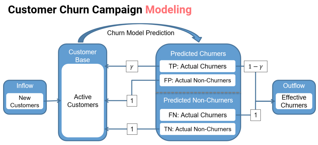
Using a churn model, those customers more likely to leave are predicted as churners and an offer is made in order to retain them. However, it is known that not all customers will accept the offer, in the case when a customer is planning to defect, it is possible that the offer is not good enough to retain him or that the reason for defecting can not be influenced by an offer. Using historical information, it is estimated that a customer will accept the offer with probability γ . On the other hand, there is the case in which the churn model misclassified a non-churner as churner, also known as false positives, in that case the customer will always accept the offer that means and additional cost to the company since those misclassified customers do not have the intentions of leaving.
In the case were the churn model predicts customers as non-churners, there is also the possibility of a misclassification, in this case an actual churner is predicted as nonchurner, since these customers do not receive an offer and they will leave the company, these cases are known as false negatives. Lastly, there is the case were the customers are actually non-churners, then there is no need to make a retention offer to these customers since they will continue to be part of the customer base.
Evaluating a churn model
From a machine learning perspective, a churn model is a classification algorithm. In the sense that using historical information, a prediction of which current customers are more likely to defect, is made. This model is normally created using one of a number of well establish algorithms (Logistic regression, neural networks, random forests, among others) Then, the model is evaluated using measures such as misclassification error, receiver operating characteristic (ROC), Kolmogorov–Smirnov (KS) or F1Score statistics.
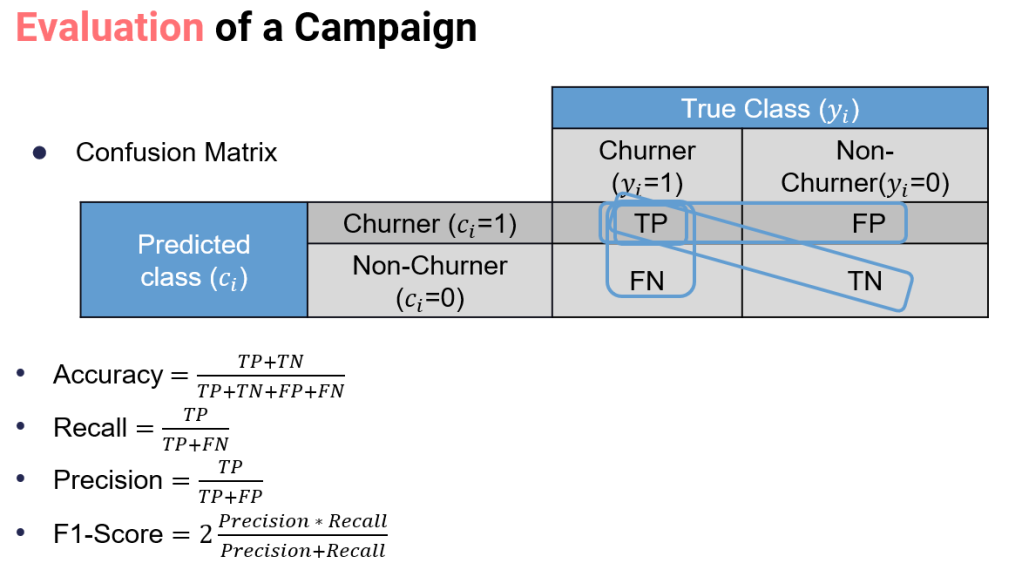
However these measures assume that misclassification errors carry the same cost, which is not the case in churn modeling, since failing to identify a profitable or unprofitable churner have significant different financial costs.
Financial evaluation of a churn model
The assumption that an error always have the same cost does not hold in the case of churn modelling, since when misidentifying a churner the financial losses are quite different than when misclassifying a non-churner as churner.
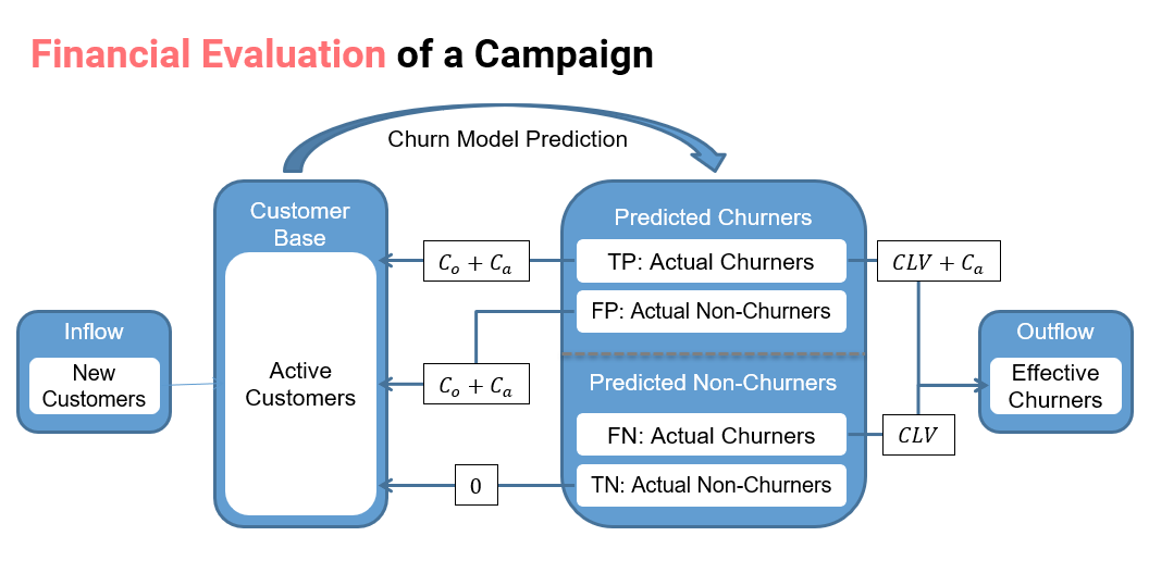
In order to obtain a more business oriented measure, we first analyze the financial impact of the different decisions, ie. false positives, false negatives, true positives and true negatives, for each customer. In the following figure, the financial impact of a churn model is shown. Note than we take into account the costs and not the profit in each case.
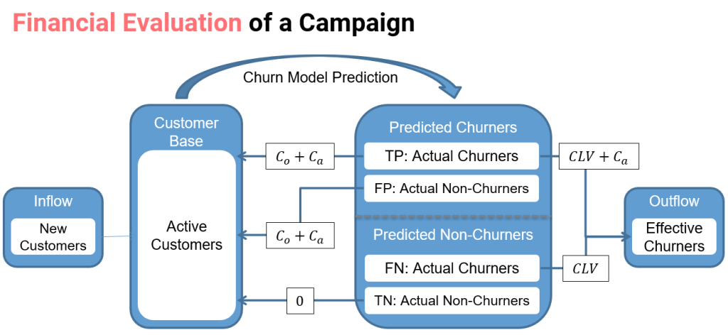
When a customer is predicted to be a churner, an offer is made with the objective of avoiding the customer defecting. However, if a customer is actually a churner, he may or not accept the offer with a probability γi. If the customer accepts the offer, the financial impact is equal to the cost of the offer (Co) plus the administrative cost of contacting the customer (Ca). On the other hand, if the customer declines the offer, the cost is the expected income that the clients would otherwise generate, also called customer lifetime value (CLV), plus Ca. Lastly, if the customer is not actually a churner, he will be happy to accept the offer and the cost will be Coi plus Ca.
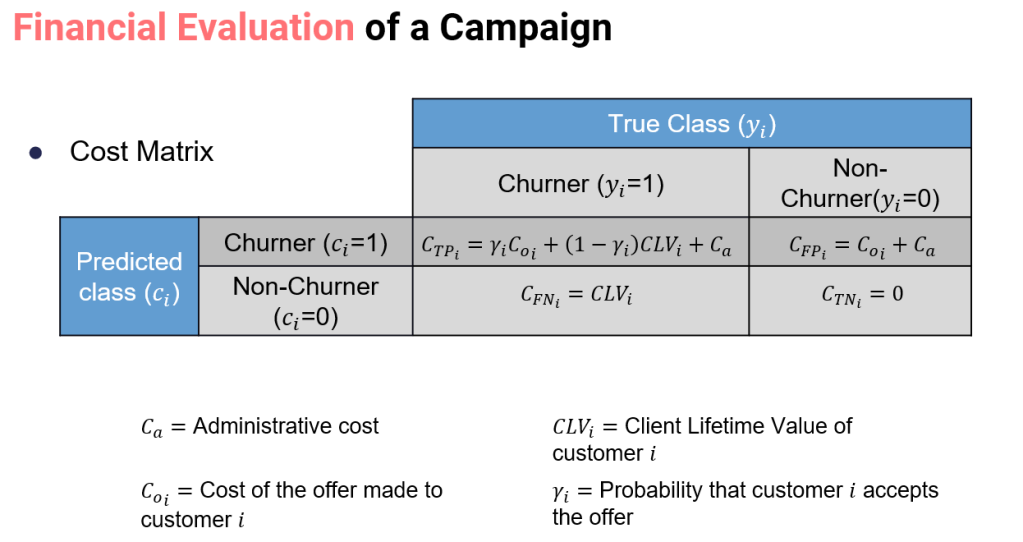
Combining the costs of each outcome with their respective probabilities, we obtain the following cost matrix.
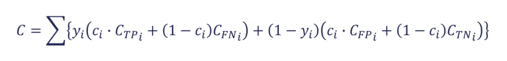
Lastly, using the cost matrix, an example-dependent cost statistic is defined
as:
And the savings are defined as:
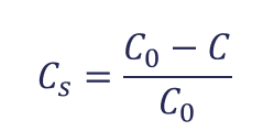
where C0 is the cost when all the customers are predicted as non-churners.
*Note: there are a couple of terms and concepts very important to understanding this methodology. For example, the customer lifetime value, or the estimation of gamma. I’ll give a deep dive in those concepts in a follow up post.
Applying the cost-sensitive framework
To showcase the performance and how to apply these concepts, we used a database of no more than 9,410 customers, each one with 45 attributes, including a churn label indicating whenever a customer is a churner. In the dataset only 455 customers are churners, leading to a churn ratio of 4.83%.
For the experiments we used three classification algorithms, decision tree, logistic regression and a random forest. Using k-fold cross validation we estimate the performance of the different algorithms using the F1-Score (traditional metric) and the Financial Savings.
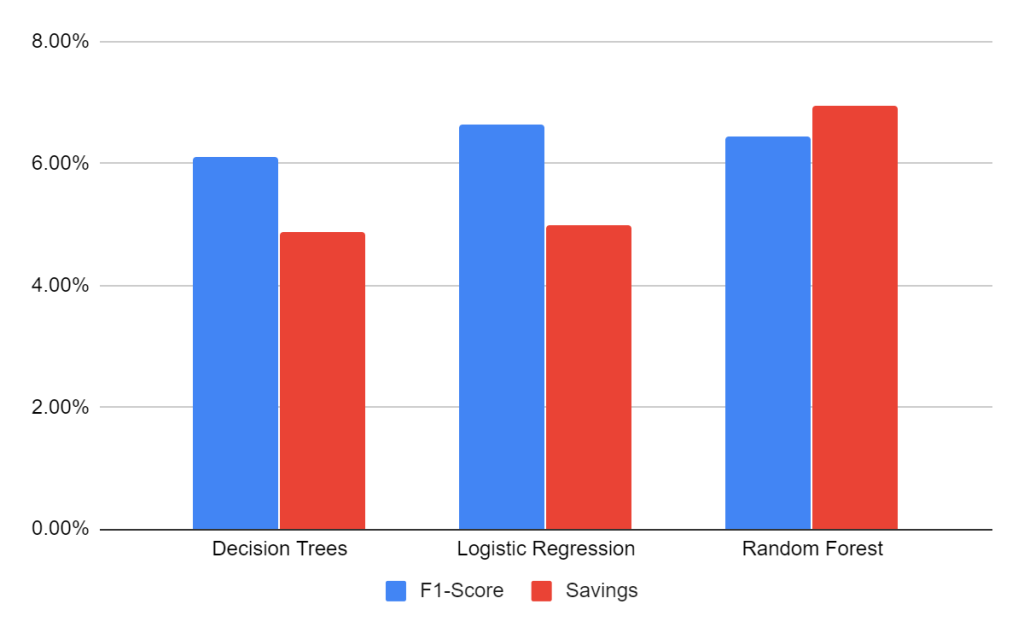
The most important highlight is that if we were using a traditional metric to select the best model, we surly would had select the Logistic Regression, however, measuring by the financial impact, the Random Forest give us much better results.
In this post we wanted to show the importance of using the actual financial costs of the churn modeling process, since there are significant differences in the results when evaluating a churn campaign using a traditional such as the F1-Score, than when using a measure that incorporates the actual financial costs such as the savings. Moreover, we also show the importance of having a measure that differentiates the costs within customers, since different customers have quite different financial impact as measured by their lifetime value.
In a following post we’re planing to discuss how to incorporate the financial costs not only when evaluating the algorithm but also during training. Also, there are important concepts such as Customer Lifetime Value and the estimation of Gamma which are important to make this methodology usable.
