Introduction
Neural networks are an example of composable systems, so it’s no surprise that they can be modeled in category theory, which is the ultimate science of composition. Moreover, the categorical ideas behind neural networks can be immediately implemented and tested in a programming language. In this post I will present the Haskell implementation of parametric lenses, generalize them to pre-lenses and introduce their profunctor representation. Using the profunctor representation I will build a working multi-layer perceptron.
In the second part of this post I will introduce the bicategory  of pre-lenses and the bicategory of triple Tambara profunctors and show how they related to pre-lenses.
Complete Haskell implementation is available on gitHub, where you can also find the PDF version of this post, complete with the categorical picture.
Haskell Implementation
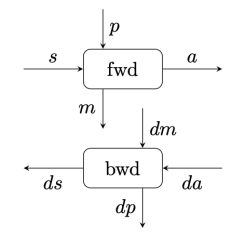
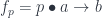
Every component of a neural network can be thought of as a system that transform input to output, and whose action depends on some parameters. In the language of neural networsks, this is called the forward pass. It takes a bunch of parameters p, combines it with the input s, and produces the output a. It can be described by a Haskell function:
fwd :: (p, s) -> a
But the real power of neural networks is in their ability to learn from mistakes. If we don’t like the output of the network, we can nudge it towards a better solution. If we want to nudge the output by some da, what change dp to the parameters should we make? The backward pass partitions the blame for the perceived error in direct proportion to the impact each parameter had on the result.
Because neural networks are composed of layers of neurons, each with their own sets or parameters, we might also ask the question: What change ds to this layer’s inputs (which are the outputs of the previous layer) should we make to improve the result? We could then back-propagate this information to the previous layer and let it adjust its own parameters. The backward pass can be described by another Haskell function:
bwd :: (p, s, da) -> (dp, ds)
The combination of these two functions forms a parametric lens:
data PLens a da p dp s ds =
PLens { fwd :: (p, s) -> a
, bwd :: (p, s, da) -> (dp, ds) }
In this representation it’s not immediately obvious how to compose parametric lenses, so I’m going to present a variety of other representations that may be more convenient in some applications.
Existential Parametric Lens
Notice that the backward pass re-uses the arguments (p, s) of the forward pass. Although some information from the forward pass is needed for the backward pass, it’s not always clear that all of it is required. It makes more sense for the forward pass to produce some kind of a care package to be delivered to the backward pass. In the simplest case, this package would just be the pair (p, s). But from the perspective of the user of the lens, the exact type of this package is an internal implementation detail, so we might as well hide it as an existential type m. We thus arrive at a more symmetric representation:
data ExLens a da p dp s ds =
  forall m . ExLens ((p, s)  -> (m, a))
                    ((m, da) -> (dp, ds))
The type m is often called the residue of the lens.
These existential lenses can be composed in series. The result of the composition is parameterized by the product (a tuple) of the original parameters. We’ll see it more clearly in the next section.
But since the product of types is associative only up to isomorphism, the composition of parametric lenses is associative only up to isomorphism.
There is also an identity lens:
identityLens :: ExLens a da () () a da
identityLens = ExLens id id
but, again, the categorical identity laws are satisfied only up to isomorphism. This is why parametric lenses cannot be interpreted as hom-sets in a traditional category. Instead they are part of a bicategory that arises from the  construction.
Pre-Lenses
Notice that there is still an asymmetry in the treatment of the parameters and the residues. The parameters are accumulated (tupled) during composition, while the residues are traced over (categorically, an existential type is described by a coend, which is a generalized trace). There is no reason why we shouldn’t accumulate the residues during composition and postpone the taking of the trace untill the very end.
We thus arrive at a fully symmetrical definition of a pre-lens:
data PreLens a da m dm p dp s ds =
  PreLens ((p, s)   -> (m, a))
          ((dm, da) -> (dp, ds))
We now have two separate types: m describing the residue, and dm describing the change of the residue.
If all we need at the end is to trace over the residues, we’ll identify the two types.
Notice that the role of parameters and residues is reversed between the forward and the backward pass. The forward pass, given the parameters and the input, produces the output plus the residue. The backward pass answers the question: How should we nudge the parameters and the inputs (dp, ds) if we want the residues and the outputs to change by (dm, da). In neural networks this will be calculated using gradient descent.
The composition of pre-lenses accumulates both the parameters and the residues into tuples:
preCompose ::
    PreLens a' da' m dm p dp s ds ->
    PreLens a da n dn q dq a' da' ->
    PreLens a da (m, n) (dm, dn) (q, p) (dq, dp) s ds
preCompose (PreLens f1 g1) (PreLens f2 g2) = PreLens f3 g3
  where
    f3 = unAssoc . second f2 . assoc . first sym .
         unAssoc . second f1 . assoc
    g3 = unAssoc . second g1 . assoc . first sym .
         unAssoc . second g2 . assoc
We use associators and symmetrizers to rearrange various tuples. Notice the separation of forward and backward passes. In particular, the backward pass of the composite lens depends only on backward passes of the composed lenses.
There is also an identity pre-lens:
idPreLens :: PreLens a da () () () () a da
idPreLens = PreLens id id
Pre-lenses thus form a bicategory that combines the and the  constructions in one.
There is also a monoidal structure in this category induced by parallel composition. In parallel composition we tuple the respective inputs and outputs, as well as the parameters and residues, both in the forward and the backward passes.
The existential lens can be obtained from the pre-lens at any time by tracing over the residues:
data ExLens a da p dp s ds =
  forall m. ExLens (PreLens a da m m p dp s ds)
Notice however that the tracing can be performed after we are done with all the (serial and parallel) compositions. In particular, we could dedicate one pipeline to perform forward passes, gathering both parameters and residues, and then send this data over to another pipeline that performs backward passes. The data is produced and consumed in the LIFO order.
Pre-Neuron
As an example, let’s implement the basic building block of neural networks, the neuron. In what follows, we’ll use the following type synonyms:
type D = Double
type V = [D]
A neuron can be decomposed into three mini-layers. The first layer is the linear transformation, which calculates the scalar product of the input vector and the vector of parameters:
It also produces the residue which, in this case, consists of the tuple (V, V) of inputs and parameters:
fw :: (V, V) -> ((V, V), D)
fw (p, s) = ((s, p), sumN n $ zipWith (*) p s)
The backward pass has the general signature:
bw :: ((dm, da) -> (dp, ds))
Because we’re eventually going to trace over the residues, we’ll use the same type for dm as for m. And because we are going to do arithmetic over the parameters, we reuse the type of p for the delta dp. Thus the signature of the backward pass is:
bw :: ((V, V), D) -> (V, V)
In the backward pass we’ll encode the gradient descent. The steepest gradient direction and slope is given by the partial derivatives:


We multiply them by the desired change in the output da:
dp = fmap (da *) s
ds = fmap (da *) p
Here’s the resulting lens:
linearL :: Int -> PreLens D D (V, V) (V, V) V V V V
linearL n = PreLens fw bw
  where
    fw :: (V, V) -> ((V, V), D)
    fw (p, s) = ((s, p), sumN n $ zipWith (*) p s)
    bw :: ((V, V), D) -> (V, V)
    bw ((s, p), da) = (fmap (da *) s
                      ,fmap (da *) p)
The linear transformation is followed by a bias, which uses a single number as the parameter, and generates no residue:
biasL :: PreLens D D () () D D D D
biasL = PreLens fw bw
  where
    fw :: (D, D) -> ((), D)
    fw (p, s) = ((), p + s)
    -- da/dp = 1, da/ds = 1
    bw :: ((), D) -> (D, D)
    bw (_, da) = (da, da)
Finally, we implement the non-linear activation layer using the tanh function:
activL :: PreLens D D D D () () D D
activL = PreLens fw bw
  where
    fw (_, s) = (s, tanh s)
    -- da/ds = 1 + (tanh s)^2
    bw (s, da)= ((), da * (1 - (tanh s)^2))
A neuron with  inputs is a composition of the three components, modulo some monoidal rearrangements:
neuronL :: Int ->
    PreLens D D ((V, V), D) ((V, V), D) Para Para V V
neuronL mIn = PreLens f' b'
  where
    PreLens f b =
      preCompose (preCompose (linearL mIn) biasL) activL
    f' :: (Para, V) -> (((V, V), D), D)
    f' (Para bi wt, s) = let (((vv, ()), d), a) =
        f (((), (bi, wt)), s)
                         in ((vv, d), a)
    b' :: (((V, V), D), D) -> (Para, V)
    b' ((vv, d), da) = let (((), (d', w')), ds) =
        b (((vv, ()), d), da)
                       in (Para d' w', ds)
The parameters for the neuron can be conveniently packaged into one data structure:
data Para = Para { bias   :: D
                 , weight :: V }

mkPara (b, v) = Para b v
unPara p = (bias p, weight p)
Using parallel composition, we can create whole layers of neurons, and then use sequential composition to model multi-layer neural networks. The loss function that compares the actual output with the expected output can also be implemented as a lens. We’ll perform this construction later using the profunctor representation.
Tambara Modules
As a rule, all optics that have an existential representation also have some kind of profunctor representation. The advantage of profunctor representations is that they are functions, and they compose using function composition.
Lenses, in particular, have a representation using a special category of profunctors called Tambara modules. A vanilla Tambara module is a profunctor p equipped with a family of transformations. It can be implemented as a Haskell class:
class  Profunctor p => Tambara p where
  alpha :: forall a da m. p a da -> p (m, a) (m, da)
The vanilla lens is then represented by the following profunctor-polymorphic function:
type Lens a da s ds = forall p. Tambara p => p a da -> p s ds
A similar representation can be constructed for pre-lenses. A pre-lens, however, has additional dependency on parameters and residues, so the analog of a Tambara module must also be parameterized by those. We need, therefore, a more complex type constructor t that takes six arguments:
t m dm p dp s ds
This is supposed to be a profunctor in three pairs of arguments, s ds, p dp, and dm m. Pro-functoriality in the first two pairs is implemented as two functions, diampS and dimapP. The inverted order in dm m means that t is covariant in m and contravariant in dm, as seen in the unusual type signature of dimapM:
dimapM  :: (m -> m') -> (dm' -> dm) ->
  t m dm p dp s ds -> t m' dm' p  dp  s  ds
To generalize Tambara modules we first observe that the pre-lens now has two independent residues, m and dm, and the two should transform separately. Also, the composition of pre-lenses accumulates (through tupling) both the residues and the parameters, so it makes sense to use the additional type arguments to TriProFunctor as accumulators. Thus the generalized Tambara module has two methods, one for accumulating residues, and one for accumulating parameters:
class TriProFunctor t => Trimbara t where
  alpha :: t m dm p dp s ds ->
           t (m1, m) (dm1, dm) p dp (m1, s) (dm1, ds)
  beta  :: t m dm p dp (p1, s) (dp1, ds) ->
           t m dm (p, p1) (dp, dp1) s ds
These generalized Tambara modules satisfy some coherency conditions.
One can also define natural transformations that are compatible with the new structures, so that Trimbara modules form a category.
The question arises: can this definition be satisfied by an actual non-trivial TriProFunctor? Fortunately, it turns out that a pre-lens itself is an example of a Trimbara module. Here’s the implementation of alpha for a PreLens:
alpha (PreLens fw bw) = PreLens fw' bw'
  where
    fw' (p, (n, s)) = let (m, a) = fw (p, s)
                      in ((n, m), a)
    bw' ((dn, dm), da) = let (dp, ds) = bw (dm, da)
                         in (dp, (dn, ds))
and this is beta:
beta (PreLens fw bw) = PreLens fw' bw'
  where
    fw' ((p, r), s) = let (m, a) = fw (p, (r, s))
                      in (m, a)
    bw' (dm, da) = let (dp, (dr, ds)) = bw (dm, da)
                   in ((dp, dr), ds)
This result will become important in the next section.
TriLens
Since Trimbara modules form a category, we can define a polymorphic function type (a categorical end) over Trimbara modules . This gives us the (tri-)profunctor representation for a pre-lens:
type TriLens a da m dm p dp s ds =
    forall t. Trimbara t => forall p1 dp1 m1 dm1.
      t m1 dm1 p1 dp1 a da ->
      t (m, m1) (dm, dm1) (p1, p) (dp1, dp) s ds
Indeed, given a pre-lens we can construct the requisite mapping of Trimbara modules simply by lifting the two functions (the forward and the backward pass) and sandwiching them between the two Tambara structure maps:
toTamb :: PreLens a da m dm p dp s ds ->
    TriLens a da m dm p dp s ds
toTamb (PreLens fw bw) = beta . dimapS fw bw . alpha
Conversely, given a mapping between Trimbara modules, we can construct a pre-lens by applying it to the identity pre-lens (modulo some rearrangement of tuples using the monoidal right/left unit laws):
fromTamb :: TriLens a da m dm p dp s ds ->
    PreLens a da m dm p dp s ds
fromTamb f = dimapM runit unRunit $
             dimapP unLunit lunit $
             f idPreLens
The main advantage of the profunctor representation is that we can now compose two lenses using simple function composition; again, modulo some associators:
triCompose ::
    TriLens b db m dm p dp s ds ->
    TriLens a da n dn q dq b db ->
    TriLens a da (m, n) (dm, dn) (q, p) (dq, dp) s ds
triCompose f g = dimapP unAssoc assoc .
                 dimapM unAssoc assoc .
                 f . g
Parallel composition of TriLenses is also relatively straightforward, although it involves a lot of bookkeeping (see the gitHub implementation).
Training a Neural Network
As a proof of concept, I have implemented and trained a simple 3-layer perceptron.
The starting point is the conversion of the individual components of the neuron from their pre-lens representation to the profunctor representation using toTamb. For instance:
linearT :: Int -> TriLens D D (V, V) (V, V) V V V V
linearT n = toTamb (linearL n)
We get a profunctor representation of a neuron by composing its three components:
neuronT :: Int ->
  TriLens D D ((V, V), D) ((V, V), D) Para Para V V
neuronT mIn =
  dimapP (second (unLunit . unPara))
         (second (mkPara . lunit)) .
  triCompose (dimapM (first runit) (first unRunit) .
  triCompose (linearT mIn) biasT) activT
With parallel composition of tri-lenses, we can build a layer of neurons of arbitrary width.
layer :: Int -> Int ->
  TriLens V V [((V, V), D)] [((V, V), D)] [Para] [Para] V V
layer mIn nOut =
  dimapP (second unRunit) (second runit) .
  dimapM (first lunit) (first unLunit) .
  triCompose (branch nOut) (vecLens nOut (neuronT mIn))
The result is again a tri-lens, and such tri-lenses can be composed in series to create a multi-layer perceptron.
makeMlp :: Int -> [Int] ->
  TriLens V V -- output
          [[((V, V), D)]] [[((V, V), D)]] -- residues
          [[Para]] [[Para]] -- parameters
          V V -- input
Here, the first integer specifies the number of inputs of each neuron in the first layer. The list [Int] specifies the number of neurons in consecutive layers (which is also the number of inputs of each neuron in the following layer).
The training of a neural network is usually done by feeding it a batch of inputs together with a batch of expected outputs. This can be simply done by arranging multiple perceptrons in parallel and accumulating the parameters for the whole batch.
batchN :: (VSpace dp) => Int ->
    TriLens  a da m dm p dp s ds ->
    TriLens [a] [da] [m] [dm] p dp [s] [ds]
To make the accumulation possible, the parameters must form a vector space, hence the constraint VSpace dp.
The whole thing is then capped by a square-distance loss lens that is parameterized by the ground truth values:
lossL :: PreLens D D ([V], [V]) ([V], [V]) [V] [V] [V] [V]
lossL = PreLens fw bw
  where
    fw (gTruth, s) =
      ((gTruth, s), sqDist (concat s) (concat gTruth))
    bw ((gTruth, s), da) = (fmap (fmap negate) delta', delta')
      where
        delta' = fmap (fmap (da *)) (zipWith minus s gTruth)
In the next post I will present the categorical version of this construction.


 “consumes” its argument exactly once. This is not the whole truth, though, because we also have linear identity
  , which ostensibly does not consume
 ![\mathit{toList} \colon \text{Array} \; a \multimap \text{Ur} \, [a]](https://s0.wp.com/latex.php?latex=%5Cmathit%7BtoList%7D+%5Ccolon+%5Ctext%7BArray%7D+%5C%3B+a+%5Cmultimap+%5Ctext%7BUr%7D+%5C%2C+%5Ba%5D&bg=ffffff&fg=29303b&s=0&c=20201002)
![\mathit{fromList} \colon [a] \to (\text{Array} \; a \multimap \text{Ur} \; b) \multimap \text{Ur} \; b](https://s0.wp.com/latex.php?latex=%5Cmathit%7BfromList%7D+%5Ccolon+%5Ba%5D+%5Cto+%28%5Ctext%7BArray%7D+%5C%3B+a+%5Cmultimap+%5Ctext%7BUr%7D+%5C%3B+b%29+%5Cmultimap+%5Ctext%7BUr%7D+%5C%3B+b+&bg=ffffff&fg=29303b&s=0&c=20201002)

 .
.  cannot be decomposed into a product of two morphisms
  .
. 

 , but it leaves you with the obligation to consume both the setter
  and the focus
  is replaced by the linear function
  . It maps pairs of object to sets, and pairs of morphisms to functions. Since we are in a monoidal category, the morphisms are linear functions, but the mappings between sets are regular functions (see Appendix 1). Thus the action of the profunctor

 is itself a Tambara module, for fixed
  . To show this, let’s construct a mapping:


 . We get:
 .
.
 at
at  , the monoidal unit.
 , we construct:
 , we can apply it to the identity optic
  and obtain
  .
.


 . In Haskell, we identify the tensor product
  or
or  . Consequently, there is no diagonal map
  , and the unit object
  is not terminal: there is no arrow
  .
. . Here,
 . Thus we have to construct:
 to
to  to arrive at
  .
.![\int_{F \colon [\mathcal C, \mathcal C]} (a \multimap F b) \to (s \multimap F t)](https://s0.wp.com/latex.php?latex=%5Cint_%7BF+%5Ccolon+%5B%5Cmathcal+C%2C+%5Cmathcal+C%5D%7D+%28a+%5Cmultimap+F+b%29+%5Cto+%28s+%5Cmultimap+F+t%29+&bg=ffffff&fg=29303b&s=0&c=20201002)
 with a set of natural transformations, written as an end over
  :
:

 . It can be written as:
 . Similarly, given two arrows
  and
and  , we can construct an arrow
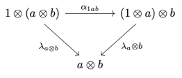
 that serves as a unit with respect to the tensor product. But, since in category theory we shy away from equalities on objects, the unit laws are not equalities, but rather natural isomorphisms, whose components are:


 with an identity natural transformation
  to get:
 . Any time you see a natural transformation tensored with an object, it’s a shorthand for whiskering.
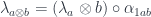


 to
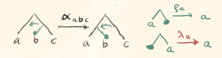
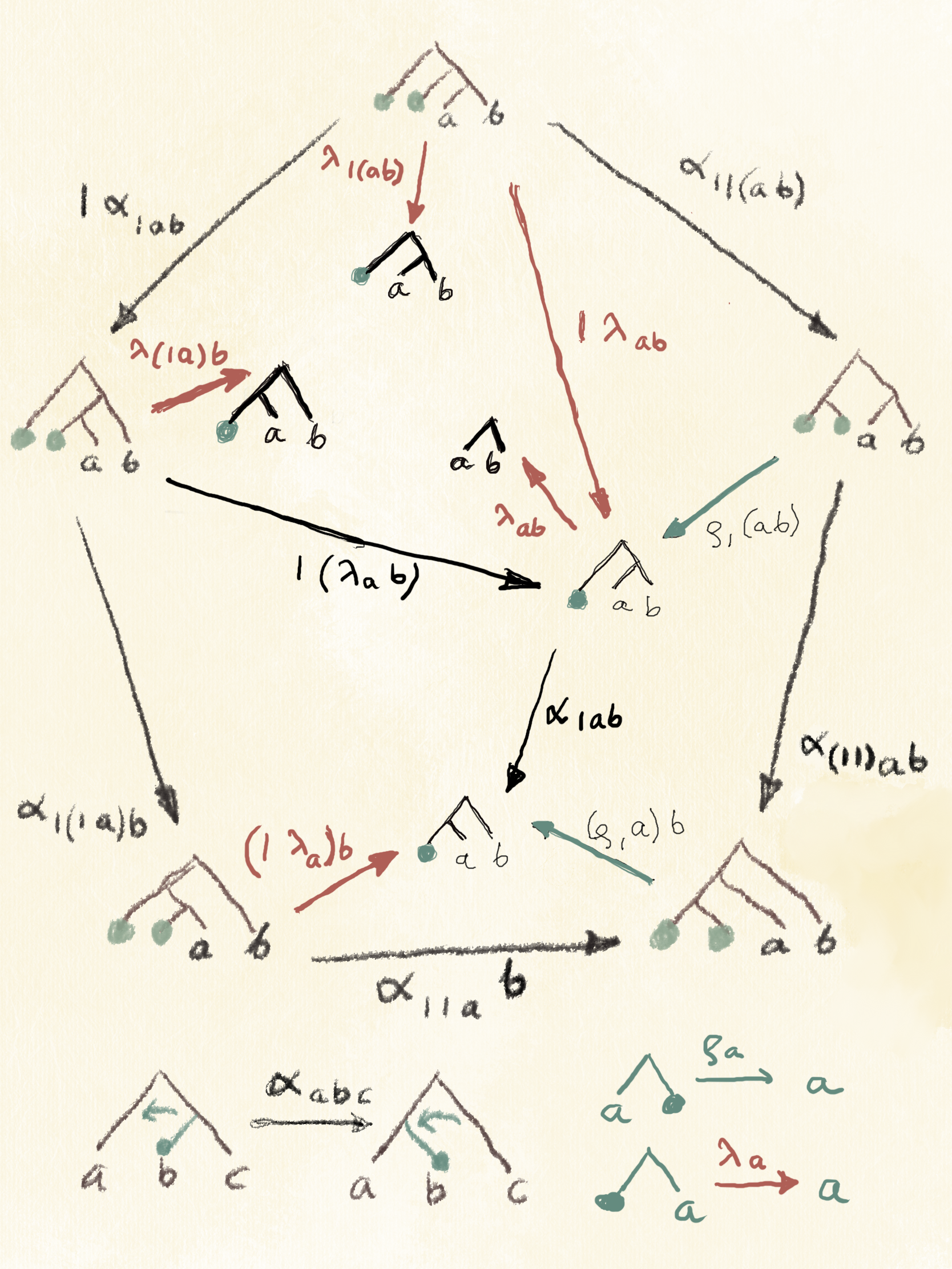
to  are equivalent. As a reminder, the notation
  at the bottom means: hold the rightmost
  in two places. But all the trees have the unit objects in the two leftmost positions, so surely he must have meant
  . I was searching for some kind of an online errata, but none was found. However, if you look closely, there are two potential sites where the right unitor could be applied, notwithstanding the fact that it has another unit to its left. So that must be it!
 . In the first case, we hold the product
  unchanged. In the second case we whisker
  with
with 
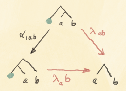
 . To apply the triangle identity, we have to do two substitutions in it. We have to use
 .
. :
:
 and
and  ; and the arrow


 . We are using its naturality in the first argument, keeping the two others constant. The arrow we are lifting is
  , and the second one to
  .
. .
.


 ) and existential quantifiers (there exists,
  ).
).

 is written as
  . The resulting optic has two possible residues,
 (I’ll use the same notation for both actions). The actions are composed using the tensor product in
 from the action of the same
 and
and  can be treated as fibers over the set
  , while the sets
  and
and  are fibers over a different set
  .
. of a discrete category
  . The products over
  are fibrated over two different sets. I have previously interpreted them as
![[\mathcal C, Set ]](https://s0.wp.com/latex.php?latex=%5B%5Cmathcal+C%2C+Set+%5D&bg=ffffff&fg=29303b&s=0&c=20201002) behaves, in many respects, like a vector space. For instance, it has a “basis” consisting of representable functors
behaves, in many respects, like a vector space. For instance, it has a “basis” consisting of representable functors  ; in the sense that any co-presheaf is as a colimit of representables. Moreover, colimit-preserving functors between co-presheaf categories are very similar to linear transformations between vector spaces. Of particular interest are functors that are left adjoint to some other functors, since left adjoints preserve colimits.
 and
and  and another with
  and
and  . Rectangular matrices
 is the transposed matrix. Transposition here serves as an analog of adjunction.
 as discrete categories. We have:
![a, b \colon [\mathcal N, \mathbf{Set}]](https://s0.wp.com/latex.php?latex=a%2C+b+%5Ccolon+%5B%5Cmathcal+N%2C+%5Cmathbf%7BSet%7D%5D+&bg=ffffff&fg=29303b&s=0&c=20201002)
![s, t \colon [\mathcal K, \mathbf{Set}]](https://s0.wp.com/latex.php?latex=s%2C+t+%5Ccolon+%5B%5Cmathcal+K%2C+%5Cmathbf%7BSet%7D%5D+&bg=ffffff&fg=29303b&s=0&c=20201002)
![c \colon [\mathcal N, \mathbf{Set}] \to [\mathcal K, \mathbf{Set}]](https://s0.wp.com/latex.php?latex=c+%5Ccolon+%5B%5Cmathcal+N%2C+%5Cmathbf%7BSet%7D%5D+%5Cto+%5B%5Cmathcal+K%2C+%5Cmathbf%7BSet%7D%5D+&bg=ffffff&fg=29303b&s=0&c=20201002)
 .
.![[\mathcal K, \mathbf{Set}] (c \bullet a, t) \cong [\mathcal N, \mathbf{Set}] (a, c^{\dagger} \bullet t)](https://s0.wp.com/latex.php?latex=%5B%5Cmathcal+K%2C+%5Cmathbf%7BSet%7D%5D+%28c+%5Cbullet+a%2C+t%29+%5Ccong+%5B%5Cmathcal+N%2C+%5Cmathbf%7BSet%7D%5D+%28a%2C+c%5E%7B%5Cdagger%7D+%5Cbullet+t%29+&bg=ffffff&fg=29303b&s=0&c=20201002)
![c^{\dagger} \colon [\mathcal K, \mathbf{Set}] \to [\mathcal N, \mathbf{Set}]](https://s0.wp.com/latex.php?latex=c%5E%7B%5Cdagger%7D+%5Ccolon+%5B%5Cmathcal+K%2C+%5Cmathbf%7BSet%7D%5D+%5Cto+%5B%5Cmathcal+N%2C+%5Cmathbf%7BSet%7D%5D+&bg=ffffff&fg=29303b&s=0&c=20201002)
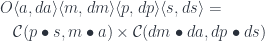
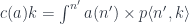
![\mathcal{O}\langle a, b\rangle \langle s, t \rangle = \int^{c} [\mathcal K, \mathbf{Set}] \left(s, c \bullet a \right) \times [\mathcal K, \mathbf{Set}] \left(c \bullet b, t \right)](https://s0.wp.com/latex.php?latex=%5Cmathcal%7BO%7D%5Clangle+a%2C+b%5Crangle+%5Clangle+s%2C+t+%5Crangle+%3D+%5Cint%5E%7Bc%7D+%5B%5Cmathcal+K%2C+%5Cmathbf%7BSet%7D%5D+%5Cleft%28s%2C++c+%5Cbullet+a+%5Cright%29+%5Ctimes+%5B%5Cmathcal+K%2C+%5Cmathbf%7BSet%7D%5D+%5Cleft%28c+%5Cbullet+b%2C+t+%5Cright%29+&bg=ffffff&fg=29303b&s=0&c=20201002)

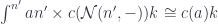
 is a representable co-presheaf.
 :
:![\int^{p} [\mathcal K, \mathbf{Set}] \left(s, \int^{n} a(n) \times p \langle n, - \rangle \right) \times [\mathcal K, \mathbf{Set}] \left(\int^{n'} b(n') \times p \langle n', - \rangle, t \right)](https://s0.wp.com/latex.php?latex=%5Cint%5E%7Bp%7D+%5B%5Cmathcal+K%2C+%5Cmathbf%7BSet%7D%5D+%5Cleft%28s%2C++%5Cint%5E%7Bn%7D+a%28n%29+%5Ctimes+p+%5Clangle+n%2C+-+%5Crangle+%5Cright%29+%5Ctimes+%5B%5Cmathcal+K%2C+%5Cmathbf%7BSet%7D%5D+%5Cleft%28%5Cint%5E%7Bn%27%7D+b%28n%27%29+%5Ctimes+p+%5Clangle+n%27%2C+-+%5Crangle%2C+t+%5Cright%29+&bg=ffffff&fg=29303b&s=0&c=20201002)
![c \colon [\mathcal N, \mathbf{Set}] \to [\mathcal K, \mathbf{Set}]](https://s0.wp.com/latex.php?latex=c+%5Ccolon++%5B%5Cmathcal+N%2C+%5Cmathbf%7BSet%7D%5D+%5Cto+%5B%5Cmathcal+K%2C+%5Cmathbf%7BSet%7D%5D+&bg=ffffff&fg=29303b&s=0&c=20201002)
![c' \colon [\mathcal K, \mathbf{Set}] \to [\mathcal M, \mathbf{Set}]](https://s0.wp.com/latex.php?latex=c%27+%5Ccolon++%5B%5Cmathcal+K%2C+%5Cmathbf%7BSet%7D%5D+%5Cto+%5B%5Cmathcal+M%2C+%5Cmathbf%7BSet%7D%5D+&bg=ffffff&fg=29303b&s=0&c=20201002)
 corresponding to
  is given by:

 and
and  . The first one tells us that there exists a
 ![l_c (s, a ) = [\mathcal K, \mathbf{Set}] \left(s, c \bullet a \right)](https://s0.wp.com/latex.php?latex=l_c+%28s%2C++a+%29+%3D+%5B%5Cmathcal+K%2C+%5Cmathbf%7BSet%7D%5D+%5Cleft%28s%2C++c+%5Cbullet+a+%5Cright%29+&bg=ffffff&fg=29303b&s=0&c=20201002)
![r_c (b, t) = [\mathcal K, \mathbf{Set}] \left(c \bullet b, t \right)](https://s0.wp.com/latex.php?latex=r_c+%28b%2C+t%29+%3D+%5B%5Cmathcal+K%2C+%5Cmathbf%7BSet%7D%5D+%5Cleft%28c+%5Cbullet+b%2C+t+%5Cright%29+&bg=ffffff&fg=29303b&s=0&c=20201002)
 and a pair:
![l'_{c'} (a, a' ) = [\mathcal K, \mathbf{Set}] \left(a, c' \bullet a' \right)](https://s0.wp.com/latex.php?latex=l%27_%7Bc%27%7D+%28a%2C++a%27+%29+%3D+%5B%5Cmathcal+K%2C+%5Cmathbf%7BSet%7D%5D+%5Cleft%28a%2C++c%27+%5Cbullet+a%27+%5Cright%29+&bg=ffffff&fg=29303b&s=0&c=20201002)
![r'_{c'} (b', b) = [\mathcal K, \mathbf{Set}] \left(c' \bullet b', b \right)](https://s0.wp.com/latex.php?latex=r%27_%7Bc%27%7D+%28b%27%2C+b%29+%3D+%5B%5Cmathcal+K%2C+%5Cmathbf%7BSet%7D%5D+%5Cleft%28c%27+%5Cbullet+b%27%2C+b+%5Cright%29+&bg=ffffff&fg=29303b&s=0&c=20201002)
 . Indeed, we can construct such an optic using the composition

![a \colon [\mathcal N, \mathbf{Set}]](https://s0.wp.com/latex.php?latex=a+%5Ccolon+%5B%5Cmathcal+N%2C+%5Cmathbf%7BSet%7D%5D+&bg=ffffff&fg=29303b&s=0&c=20201002)

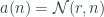

 :
:

![\partial_{[\rho} F_{\mu \nu ]} = 0](https://s0.wp.com/latex.php?latex=%5Cpartial_%7B%5B%5Crho%7D+F_%7B%5Cmu+%5Cnu+%5D%7D+%3D+0&bg=ffffff&fg=29303b&s=0&c=20201002)
 called the vector potential. The field tensor can be expressed as its anti-symmetrized derivative
![F_{\mu \nu} = \partial_{[ \mu} A_{\nu ]}](https://s0.wp.com/latex.php?latex=F_%7B%5Cmu+%5Cnu%7D+%3D+%5Cpartial_%7B%5B+%5Cmu%7D+A_%7B%5Cnu+%5D%7D&bg=ffffff&fg=29303b&s=0&c=20201002)
![\partial_{[\rho} F_{\mu \nu ]} = \partial_{[\rho} \partial_{ \mu} A_{\nu ]} = 0](https://s0.wp.com/latex.php?latex=%5Cpartial_%7B%5B%5Crho%7D+F_%7B%5Cmu+%5Cnu+%5D%7D+%3D+%5Cpartial_%7B%5B%5Crho%7D+%5Cpartial_%7B+%5Cmu%7D+A_%7B%5Cnu+%5D%7D+%3D+0&bg=ffffff&fg=29303b&s=0&c=20201002)
 .
. as its curvature. The second Maxwell equation is the Bianchi identity for this connection.
 is a completely arbitrary, time dependent scalar field. This is, again, because of the symmetry of partial derivatives:
![F_{\mu \nu}' = \partial_{[ \mu} A'_{\nu ]} = \partial_{[ \mu} A_{\nu ]} + \partial_{[ \mu} \partial_{\nu ]} \Lambda = \partial_{[ \mu} A_{\nu ]} = F_{\mu \nu}](https://s0.wp.com/latex.php?latex=F_%7B%5Cmu+%5Cnu%7D%27+%3D+%5Cpartial_%7B%5B+%5Cmu%7D+A%27_%7B%5Cnu+%5D%7D+%3D+%5Cpartial_%7B%5B+%5Cmu%7D+A_%7B%5Cnu+%5D%7D+%2B+%5Cpartial_%7B%5B+%5Cmu%7D+%5Cpartial_%7B%5Cnu+%5D%7D+%5CLambda+%3D+%5Cpartial_%7B%5B+%5Cmu%7D+A_%7B%5Cnu+%5D%7D+%3D+F_%7B%5Cmu+%5Cnu%7D&bg=ffffff&fg=29303b&s=0&c=20201002)
 is called a gauge transformation, and we can formulated a new law: Physics in invariant under gauge transformations. There is a beautiful symmetry we have discovered in nature.
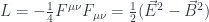

 . This is all the information about matter that the fields need to know. In fact, this equation imposes additional constraints on the matter. If you differentiate it once more, you get:
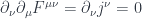


 . The problem is that two such paths that differ only by a gauge transformation result in exactly the same action, since the Lagrangian is written in terms of gauge invariant fields
  in the electromagnetic field is:
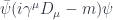
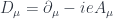
 is the electron charge.
 (the
(the  , the phases cancel, which shows that the Lagrangian does not depend on the choice of the phase.


 . Such potential is called pure gauge, because it can be “gauged away” using
  .
.

 , where
  is the time coordinate, and the rest are space coordinates. We use the system of units in which the speed of light
 ![F_{0 1} = \partial_{[0} A_{1]} = \partial_{0} A_{1} - \partial_{1} A_{0} = \partial_{t} A_{x} - \partial_{x} A_{t}](https://s0.wp.com/latex.php?latex=F_%7B0+1%7D+%3D+%5Cpartial_%7B%5B0%7D+A_%7B1%5D%7D+%3D+%5Cpartial_%7B0%7D+A_%7B1%7D+-+%5Cpartial_%7B1%7D+A_%7B0%7D+%3D+%5Cpartial_%7Bt%7D+A_%7Bx%7D+-+%5Cpartial_%7Bx%7D+A_%7Bt%7D&bg=ffffff&fg=29303b&s=0&c=20201002)


 matrix, but because of antisymmetry, it reduces to just 6 independent entries, which can be rearranged into two 3-d vector fields. The vector
  is the electric field, and the vector
  is the magnetic field.
 . Its zeroth component describes the distribution of electric charges, and the rest describes electric current density.
 that consists of polynomial functors in which the fibration is done over one fixed set


 . In this setting, we’ll write the residues
  as profunctors:

 . (Incidentally, a monoid in this category is called a promonad.)
 .
.
![[\mathcal{N}, \mathbf{Set}]](https://s0.wp.com/latex.php?latex=%5B%5Cmathcal%7BN%7D%2C+%5Cmathbf%7BSet%7D%5D+&bg=ffffff&fg=29303b&s=0&c=20201002) .
.![\mathbf{Pl}\langle s, t\rangle \langle a, b\rangle \cong \int^{c \colon [\mathcal{N}^{op} \times \mathcal{N}, Set]} [\mathcal{N}, \mathbf{Set}] \left(s, c \bullet a\right) \times [\mathcal{N}, \mathbf{Set}] \left(c \bullet b, t\right)](https://s0.wp.com/latex.php?latex=%5Cmathbf%7BPl%7D%5Clangle+s%2C+t%5Crangle+%5Clangle+a%2C+b%5Crangle+%5Ccong+%5Cint%5E%7Bc+%5Ccolon+%5B%5Cmathcal%7BN%7D%5E%7Bop%7D+%5Ctimes+%5Cmathcal%7BN%7D%2C+Set%5D%7D+++%5B%5Cmathcal%7BN%7D%2C+%5Cmathbf%7BSet%7D%5D++%5Cleft%28s%2C+c+%5Cbullet+a%5Cright%29++%5Ctimes++%5B%5Cmathcal%7BN%7D%2C+%5Cmathbf%7BSet%7D%5D++%5Cleft%28c+%5Cbullet+b%2C+t%5Cright%29+&bg=ffffff&fg=29303b&s=0&c=20201002)


![\cong \int_{n, k} \mathbf{Set}\left(c\langle k, n \rangle , [b(k), t (n)]\right)](https://s0.wp.com/latex.php?latex=%5Ccong+++%5Cint_%7Bn%2C+k%7D+%5Cmathbf%7BSet%7D%5Cleft%28c%5Clangle+k%2C+n+%5Crangle+%2C+%5Bb%28k%29%2C+t+%28n%29%5D%5Cright%29+&bg=ffffff&fg=29303b&s=0&c=20201002)
 , is:
, is:![\mathbf{Pl}\langle s, t\rangle \langle a, b\rangle \cong \int_m \mathbf{Set}\left(s(m), \int^j a(j) \times [b(j), t(m)] \right)](https://s0.wp.com/latex.php?latex=%5Cmathbf%7BPl%7D%5Clangle+s%2C+t%5Crangle+%5Clangle+a%2C+b%5Crangle+%5Ccong+%5Cint_m+%5Cmathbf%7BSet%7D%5Cleft%28s%28m%29%2C+%5Cint%5Ej+a%28j%29+%5Ctimes+%5Bb%28j%29%2C+t%28m%29%5D+%5Cright%29&bg=ffffff&fg=29303b&s=0&c=20201002)
![[\mathcal{N}, \mathbf{Set}] ( s, [b, t] \bullet a)](https://s0.wp.com/latex.php?latex=%5B%5Cmathcal%7BN%7D%2C+%5Cmathbf%7BSet%7D%5D+%28+s%2C+%5Bb%2C+t%5D+%5Cbullet+a%29&bg=ffffff&fg=29303b&s=0&c=20201002)
 of profunctors of the type:
![P \colon [\mathcal{N}, \mathbf{Set}]^{op} \times [\mathcal{N}, \mathbf{Set}] \to \mathbf{Set}](https://s0.wp.com/latex.php?latex=P+%5Ccolon+%5B%5Cmathcal%7BN%7D%2C+%5Cmathbf%7BSet%7D%5D%5E%7Bop%7D++%5Ctimes+%5B%5Cmathcal%7BN%7D%2C+%5Cmathbf%7BSet%7D%5D+%5Cto+%5Cmathbf%7BSet%7D+&bg=ffffff&fg=29303b&s=0&c=20201002)


 is the obvious forgetful functor from
 ![\mathbf{PolyLens}\langle s, t\rangle \langle a, b\rangle = \prod_{k} \mathbf{Set}\left(s_k, \sum_{n} a_n \times [b_n, t_k] \right)](https://s0.wp.com/latex.php?latex=%5Cmathbf%7BPolyLens%7D%5Clangle+s%2C+t%5Crangle+%5Clangle+a%2C+b%5Crangle+%3D+%5Cprod_%7Bk%7D+%5Cmathbf%7BSet%7D%5Cleft%28s_k%2C+%5Csum_%7Bn%7D+a_n+%5Ctimes+%5Bb_n%2C+t_k%5D+%5Cright%29+&bg=ffffff&fg=29303b&s=0&c=20201002)
 stands for a set of functions from
 ![[a, b]](https://s0.wp.com/latex.php?latex=%5Ba%2C+b%5D&bg=ffffff&fg=29303b&s=0&c=20201002) (the internal hom is the same as the external hom in
(the internal hom is the same as the external hom in  is the type of pairs
 ![\sum_{n} a_n \times [b_n, t_k]](https://s0.wp.com/latex.php?latex=%5Csum_%7Bn%7D+a_n+%5Ctimes+%5Bb_n%2C+t_k%5D+&bg=ffffff&fg=29303b&s=0&c=20201002)
 and
and  are indexed by elements of the set
  and
and  over
over 
![[t_n, y]](https://s0.wp.com/latex.php?latex=%5Bt_n%2C+y%5D&bg=ffffff&fg=29303b&s=0&c=20201002) for the internal hom:
for the internal hom:![P(y) = \sum_{n \in N} s_n \times [t_n, y]](https://s0.wp.com/latex.php?latex=P%28y%29+%3D+%5Csum_%7Bn+%5Cin+N%7D+s_n+%5Ctimes+%5Bt_n%2C+y%5D+&bg=ffffff&fg=29303b&s=0&c=20201002)
 and
and  . A natural transformation between them can be written as an end. Let’s first expand the source functor:
![\mathbf{Poly}\left( \sum_k s_k \times [t_k, -], Q\right) = \int_{y\colon \mathbf{Set}} \mathbf{Set} \left(\sum_k s_k \times [t_k, y], Q(y)\right)](https://s0.wp.com/latex.php?latex=%5Cmathbf%7BPoly%7D%5Cleft%28+%5Csum_k+s_k+%5Ctimes+%5Bt_k%2C+-%5D%2C+Q%5Cright%29++%3D++%5Cint_%7By%5Ccolon+%5Cmathbf%7BSet%7D%7D+%5Cmathbf%7BSet%7D+%5Cleft%28%5Csum_k+s_k+%5Ctimes+%5Bt_k%2C+y%5D%2C+Q%28y%29%5Cright%29&bg=ffffff&fg=29303b&s=0&c=20201002)
![\cong \prod_k \int_y \mathbf{Set} \left(s_k \times [t_k, y], Q(y)\right)](https://s0.wp.com/latex.php?latex=%5Ccong+%5Cprod_k+%5Cint_y+%5Cmathbf%7BSet%7D+%5Cleft%28s_k+%5Ctimes+%5Bt_k%2C+y%5D%2C+Q%28y%29%5Cright%29+&bg=ffffff&fg=29303b&s=0&c=20201002)
![\int_y \mathbf{Set} \left( s \times [t, y], \sum_n a_n \times [b_n, y]\right)](https://s0.wp.com/latex.php?latex=%5Cint_y+%5Cmathbf%7BSet%7D+%5Cleft%28+s+%5Ctimes+%5Bt%2C+y%5D%2C+%5Csum_n+a_n+%5Ctimes+%5Bb_n%2C+y%5D%5Cright%29+&bg=ffffff&fg=29303b&s=0&c=20201002)
![\int_y \mathbf{Set} \left( [t, y], \left[s, \sum_n a_n \times [b_n, y]\right] \right)](https://s0.wp.com/latex.php?latex=%5Cint_y+%5Cmathbf%7BSet%7D+%5Cleft%28+%5Bt%2C+y%5D%2C++%5Cleft%5Bs%2C+%5Csum_n+a_n+%5Ctimes+%5Bb_n%2C+y%5D%5Cright%5D++%5Cright%29+&bg=ffffff&fg=29303b&s=0&c=20201002)
![\int_y \mathbf{Set} \left( \mathbf{Set}(t, y), \mathbf{Set} \left(s, \sum_n a_n \times [b_n, y]\right) \right)](https://s0.wp.com/latex.php?latex=%5Cint_y+%5Cmathbf%7BSet%7D+%5Cleft%28+%5Cmathbf%7BSet%7D%28t%2C+y%29%2C+%5Cmathbf%7BSet%7D+%5Cleft%28s%2C+%5Csum_n+a_n+%5Ctimes+%5Bb_n%2C+y%5D%5Cright%29++%5Cright%29+&bg=ffffff&fg=29303b&s=0&c=20201002)
 with
with ![\mathbf{Set}\left(s, \sum_n a_n \times [b_n, t] \right)](https://s0.wp.com/latex.php?latex=%5Cmathbf%7BSet%7D%5Cleft%28s%2C+%5Csum_n+a_n+%5Ctimes+%5Bb_n%2C+t%5D+%5Cright%29+&bg=ffffff&fg=29303b&s=0&c=20201002)
![\sum_k s_k \times [t_k, y]](https://s0.wp.com/latex.php?latex=%5Csum_k+s_k+%5Ctimes+%5Bt_k%2C+y%5D&bg=ffffff&fg=29303b&s=0&c=20201002) and
and ![\sum_n a_n \times [b_n, y]](https://s0.wp.com/latex.php?latex=%5Csum_n+a_n+%5Ctimes+%5Bb_n%2C+y%5D&bg=ffffff&fg=29303b&s=0&c=20201002) is called a polynomial lens. Combining the previous results, we see that it can be written as:
is called a polynomial lens. Combining the previous results, we see that it can be written as:![\mathbf{PolyLens}\langle s, t\rangle \langle a, b\rangle = \prod_{k \in K} \mathbf{Set}\left(s_k, \sum_{n \in N} a_n \times [b_n, t_k] \right)](https://s0.wp.com/latex.php?latex=%5Cmathbf%7BPolyLens%7D%5Clangle+s%2C+t%5Crangle+%5Clangle+a%2C+b%5Crangle+%3D+%5Cprod_%7Bk+%5Cin+K%7D+%5Cmathbf%7BSet%7D%5Cleft%28s_k%2C+%5Csum_%7Bn+%5Cin+N%7D+a_n+%5Ctimes+%5Bb_n%2C+t_k%5D+%5Cright%29+&bg=ffffff&fg=29303b&s=0&c=20201002)
 depends not only on the type but also on the value of the argument
  .
.![Lan_b a \cong \int^{n \colon \mathcal{N}} a \times [b, -]](https://s0.wp.com/latex.php?latex=Lan_b+a+%5Ccong+%5Cint%5E%7Bn+%5Ccolon+%5Cmathcal%7BN%7D%7D+a+%5Ctimes+%5Bb%2C+-%5D+&bg=ffffff&fg=29303b&s=0&c=20201002)
 becomes a product. An end of hom-sets becomes a natural transformation. A polynomial lens can therefore be rewritten as:
![\prod_{k \in K} \mathbf{Set}\left(s_k, \sum_{n \in N} a_n \times [b_n, t_k] \right) \cong [\mathcal{K}, \mathbf{Set}](s, (Lan_b a) \circ t)](https://s0.wp.com/latex.php?latex=%5Cprod_%7Bk+%5Cin+K%7D+%5Cmathbf%7BSet%7D%5Cleft%28s_k%2C+%5Csum_%7Bn+%5Cin+N%7D+a_n+%5Ctimes+%5Bb_n%2C+t_k%5D+%5Cright%29++%5Ccong+%5B%5Cmathcal%7BK%7D%2C+%5Cmathbf%7BSet%7D%5D%28s%2C+%28Lan_b+a%29+%5Ccirc+t%29+&bg=ffffff&fg=29303b&s=0&c=20201002)
](https://s0.wp.com/latex.php?latex=%5Cmathbf%7BPolyLens%7D%5Clangle+s%2C+t%5Crangle+%5Clangle+a%2C+b%5Crangle+%5Ccong+%5B%5Cmathbf%7BSet%7D%2C+%5Cmathbf%7BSet%7D%5D%28Lan_t+s%2C+Lan_b+a%29+&bg=ffffff&fg=29303b&s=0&c=20201002)

![\prod_{i \in K} \prod_{m \in N} \mathbf{Set}\left(c_{m i}, [b_m, t_i ]\right)](https://s0.wp.com/latex.php?latex=%5Cprod_%7Bi+%5Cin+K%7D+%5Cprod_%7Bm+%5Cin+N%7D+%5Cmathbf%7BSet%7D%5Cleft%28c_%7Bm+i%7D%2C+%5Bb_m%2C+t_i+%5D%5Cright%29&bg=ffffff&fg=29303b&s=0&c=20201002)
![\prod_{i \in K} \prod_{m \in N} \mathbf{Set} \left(c_{m i}, [b_m, t_i] \right) \cong [\mathcal{N}^{op} \times \mathcal{K}, \mathbf{Set}]\left(c_{= -}, [b_=, t_- ]\right)](https://s0.wp.com/latex.php?latex=%5Cprod_%7Bi+%5Cin+K%7D+%5Cprod_%7Bm+%5Cin+N%7D+%5Cmathbf%7BSet%7D+%5Cleft%28c_%7Bm+i%7D%2C+%5Bb_m%2C+t_i%5D+%5Cright%29+%5Ccong+%5B%5Cmathcal%7BN%7D%5E%7Bop%7D+%5Ctimes+%5Cmathcal%7BK%7D%2C+%5Cmathbf%7BSet%7D%5D%5Cleft%28c_%7B%3D+-%7D%2C+%5Bb_%3D%2C+t_-+%5D%5Cright%29&bg=ffffff&fg=29303b&s=0&c=20201002)
 .
. . The result is that
  can be wrtitten as:
![\int^{c_{k i}} \prod_{k \in K} \mathbf{Set} \left(s_k, \sum_{n \in N} a_n \times c_{n k} \right) \times [\mathcal{N}^{op} \times \mathcal{K}, \mathbf{Set}]\left(c_{= -}, [b_=, t_- ]\right)](https://s0.wp.com/latex.php?latex=%5Cint%5E%7Bc_%7Bk+i%7D%7D+%5Cprod_%7Bk+%5Cin+K%7D+%5Cmathbf%7BSet%7D+%5Cleft%28s_k%2C++%5Csum_%7Bn+%5Cin+N%7D+a_n+%5Ctimes+c_%7Bn+k%7D+%5Cright%29+%5Ctimes+%5B%5Cmathcal%7BN%7D%5E%7Bop%7D+%5Ctimes+%5Cmathcal%7BK%7D%2C+%5Cmathbf%7BSet%7D%5D%5Cleft%28c_%7B%3D+-%7D%2C+%5Bb_%3D%2C+t_-+%5D%5Cright%29+&bg=ffffff&fg=29303b&s=0&c=20201002)
![\cong \prod_{k \in K} \mathbf{Set}\left(s_k, \sum_{n \in N} a_n \times [b_n, t_k] \right)](https://s0.wp.com/latex.php?latex=%5Ccong++%5Cprod_%7Bk+%5Cin+K%7D+%5Cmathbf%7BSet%7D%5Cleft%28s_k%2C+%5Csum_%7Bn+%5Cin+N%7D+a_n+%5Ctimes+%5Bb_n%2C+t_k%5D+%5Cright%29+&bg=ffffff&fg=29303b&s=0&c=20201002)

