One of my teaching roles is in an introductory Genetics course, where first year students are presented with a wide range of new ideas at a relatively fast pace. It seems that often, students choose to take a memorization approach to learning the material, rather than taking the chance to think about how and why these genetic concepts actually work. It is my conviction that, as teachers, it is our role to provide students with the opportunities to engage with the course material, and construct a solid understanding that will serve them as they proceed on to higher specialization.
When it comes to bang for my pedagogical buck, I have found that you really can’t beat the use of simulation as a platform for providing the opportunity for students to engage with theoretical concepts. Here is an R script which I have written and used to allow students to explore how random mating in a population leads to the well known Hardy-Weinberg (HW) distribution.
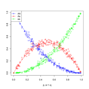
For those who need a refresher, HW describes the genotype frequencies in randomly mating population. For the simple two allele case (A >> a), the frequencies are denoted by p and q; freq(A) = p; freq(a) = q; p + q = 1. If the population is in equilibrium, then freq(AA) = p2 for the AA homozygotes in the population, freq(aa) = q2 for the aa homozygotes, and freq(Aa) = 2pq for the heterozygotes.
What doesn’t usually get mentioned in introductory courses, is that the HW formula provides the expected frequencies of each genotype. Of course, in real, finite populations, there will be variability around these values. The seeming exactness of HW obscures the random processes at play. To help students see how HW arises in finite populations (as opposed to the theoretical infinite populations required for the strict solution), I let them play with this simulation (R script).
Students can play around with the population size (N) and the number of generations (num_generations), to see how well the simulated populations correspond to the predicted HW. Here is a plot of 200 simulated populations of size N=200, which are initiated out of the HW equilibrium and then randomly mated for one generation:
Feel free to try it out in your own class!
-BayesianBiologist

Though this is out of reach of many Intro Genetics students, the beauty of H-W is how it allows us to track allele frequencies through what is assumed to be the focus of selection, that is, the genotype. Because selection (through differential viability) is easily incorporated into the H-W framework we can model evolution (as defined by changes in allele frequencies) extremely easily, providing an explicit, quantitative demonstration of evolution that is entirely concordant with Mendelian genetics.
True – the utility of HW in quantifying selection is not usually taught at the intro level. Students are usually just told that HW is what happens under no selection, mutation, or migration. Perhaps at least alluding to how it is useful in current problems would provide a little more motivation for understanding it. -Thanks for the read, Adam!
Nice idea, I’ll use it in class. 🙂
Pingback: Simulating weak gravitational lensing « bayesianbiologist
I’m trying to modify your code to depict three alleles. The code is running, but I’m not sure how to graph it with the additional variable. Any suggestions?
With three alleles you’re into higher dimensional space. You want to show the relative frequencies your 6 possible genotypes as a function of the relative frequencies of the 3 alleles. The problem is that representing the relative frequencies of three alleles requires two dimensions (since there are two degrees of freedom), and then a third on which to project the genotype frequencies. I’m picturing maybe doing it as a 6 panel figure, one for each genotype. Each panel would be a 3d plot with x=frequency of allele a, y= frequency of allele b, and z=frequency of a genotype. (note that frequency of allele c is determined by the location in the x,y plane since a+b+c=1.)
Good luck!
Thanks!
Pingback: Simudidactic | bayesianbiologist
Hi Corey,
I am extremely interested in the idea of simulation in introducing science concepts in general. I tried to open the R script that you have nice provided in the article but it does not open up. Any suggestions?
Thank you
Narmin
Thanks for pointing out the dead links, Narmin. I’ve updated them to point to the gist here https://gist.github.com/cjbayesian/468725f4bd7d6f3f027d#file-hw_sim-r
Good luck!
Hi Corey! Great post. Do you have the AA and aa labels switched around in your figure (https://biolympiads.com/population-genetics-iii/)?
I ask because I am trying to create a null distribution of expected allele frequencies to compare to my experimental allele frqeuences (example figure of distribution can be found on page 31: http://adegenet.r-forge.r-project.org/files/tutorial-genomics.pdf). I think your R script is great and am trying to convert this is a frequency distribution that includes AA, aa, and Aa.
I am using the following but I don’t think it is quite correct:
freqaa<-curve(x^2,col='darkgreen',add=T)
hist(freqaa$y, nclass=20)
freqAA<-curve((1-x)^2,col='blue',add=T)
hist(freqAA$y, nclass=20)
No longer works — looks like updated gist is broken. random_mating doesnt return nor edit pop.
Hi, i am really intrigued, where can I see the script?
https://gist.github.com/cjbayesian/468725f4bd7d6f3f027d#file-hw_sim-r