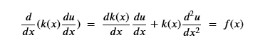
Over the last two years  some very interesting research has emerged that illustrates a fascinating connection between Deep Neural Nets and differential equations.    There are two aspects of these discoveries that will be described here.  They are

1. Many differential equations (linear, elliptical, non-linear and even stochastic PDEs) can be solved with the aid of deep neural networks.
2. Many classic deep neural networks can be seen as approximations to differential equations and modern differential equation solvers can great simplify those neural networks.

The solution of PDE by neural networks described here is largely the excellent work of Karniadakis at Brown University and his collaborators on “Physics Informed Neural Networks” (PINNs).   This work has led to some impressive theory and also advances in applications such as uncertainty quantification of the models of subsurface flow at the Hanford nuclear site, one of the most contaminated sites in the western hemisphere.

While the work on PINNs shows us how to use neural networks to solve differential equations, the second discovery cited above tells us how modern differential equation solvers can simplify the architecture of many neural networks.  A team led by Chen , Rubanova , Bettencourt, Duvenaud at the University of Toronto, Vector Institute examined the design of some neural networks and noticed how their architecture resembled discretizations of certain differential equations.  This led them to define a hybrid of neural net and differential equation they call a “Neural Ordinary Differential Equation”. Neural ODEs  have several striking properties including excellent accuracy and greatly reduced memory requirements.

These works suggest that there exists a duality between differential equations and many deep neural networks that is worth trying to understand.  This paper will not be a deep mathematical analysis, but rather, try to provide some intuition and examples (with PyTorch code).  We first describe the solution of PDEs with neural networks and then look neural ODEs.

PINNs

We now turn to the work on using neural networks to solve partial differential equations.  The examples we will study are from four papers.

1. Raissi, Perdikaris, and Karniadakis, “Physics Informed Deep Learning (Part II): Data-driven Discovery of Nonlinear Partial Differential Equations”, Nov 2017, is the paper that introduces PINNS and demonstrates the concept by showing how to solve several “classical” PDEs.
2. Yang, Zhang, and Karniadakis, “Physics-Informed Generative Adversarial Networks for Stochastic Differential Equations”, Nov 2018, addresses the problem of stochastic differential equations but uses a generative adversarial neural network.
3. Yang, et. all “Highly-scalable, physics-informed GANs for learning solutions of stochastic PDEs”, oct 2019, is the large study that applies the GAN PINNs techniques to the large scale problem of  as uncertainty quantification of the models of subsurface flow at the Hanford nuclear site.
4. Shin, Darbon and Karniadakis, “On the Convergence and Generalization of Physics Informed Neural Networks”, 2020, is the theoretical proof that the PINNs approach really works.

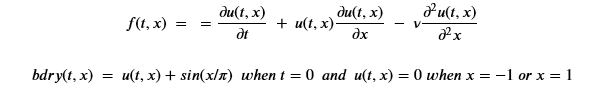
We will start with a very simple partial differ that is discussed in the Rassi paper.  Burgers’ Equation is an excellent example to study if you want to understand how shock waves can come about from relatively benign initial conditions.  The equation is

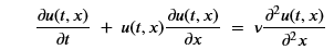
Were the domain of x is the interval [-1, 1] and the time variable t go from 0 to 1.   The initial, t=0, condition is u(0,x) = -sin(pi*x). and the boundary conditions are u(t,-1) = u(t,1)=0.  The parameter v is 0.01/pi.   (If we set v = 0 then this is the inviscid equation which does describe shock waves, but with v >0 the equation is called the viscus Burgers’ equations.  While not technically describing discontinuity shock as t goes forward in time, it is awfully close.    The figure below shows the evolution of the value of u(t,x) from the initial sine wave at t=0 to a near discontinuity at t=39.

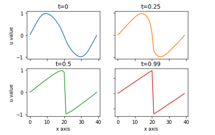
Figure 1.  Samples of u(t, x) for x in [-1,1] at 40 points and t in 4 points.

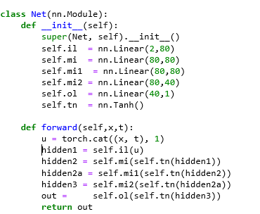
The basic idea of a physics informed neural net is,  in this case, a network defining a map

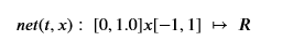
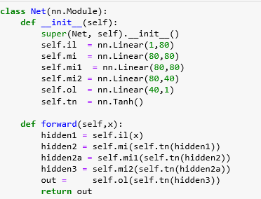
This network, when trained, should satisfy both the boundary condition and the differential equation.   To satisfy the differential equation we must be able to differentiate the network as a function of x and t.  But we know how to do that! We compute the derivatives of a network symbolically when we do the back propagation for training.   Neural nets are non-linear functions with first derivatives.   In our case we also need the second derivatives which means that we cannot use ReLU as an activation function because it is piecewise linear and has second derivatives that are all zeros.   However Tanh is smooth with fine second derivatives so we will build our net function as follows.

Our goal is to train an instance of this network to minimize the functions

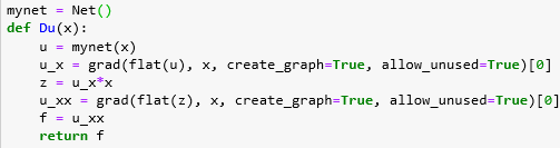
The function f in Torch is

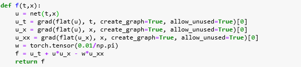
Where we are using the grad function from torch.autograd  to compute derivatives.  The function flat(x) just returns the list [x[i] for i in range(x.shape[0)].

The unique thing here is that we are training the network to satisfy the differential equation and boundary conditions without data samples from the solution u.  When converged the network should give us the solution u.  This works because Burger’s equation, in this form, has been proven to have a unique solution,  Of course, this raises the question: when are a differential equation and boundary conditions sufficient to guarantee the existence and uniqueness of a solution?  Simple linear differential operators do, but not all differential equations.  In the case of PINNs, one can speculate that if our laws of nature are correct, then nature proves the solution exists. (Thanks to Wolfgang Gentzsch and Joseph Pareti for making me realize this point needed to be made.)

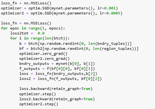
To train the network we iterate over 200000  epochs  using two optimizers (one for the boundary and one for the function differential equation function f).   For each epoch we randomly draw a batch of boundary samples and a batch of samples drawn from the interior of the [0,1]x[-1,1] rectangle.   Each sample is a tuple consisting of a t-value, an x-value and a u boundary value or zero.  (Recall we are forcing f(t, x) to zero and bndry to zero or u(0,x).)  The main part of the code is below.  The full details are in the github repository.

A python library giving us an approximation of an exact solution is available on line that we can use to compare to our result. Figure 2 below shows the heatmap of the solution.

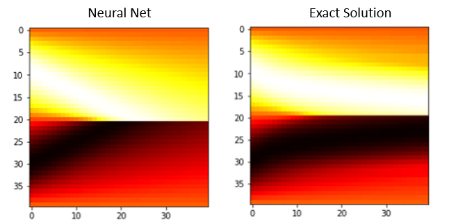
Figure 2.  The horizontal axis is time (t in [0,1]) sampled at 40 points and the vertical axis is x in the interval [-1,1] sampled at 40 points.  Dark colors are u values near 1 and white are u values near -1.

The mid horizontal line shows the evolution of the shock as it becomes a sharp transition as t goes from 0 to 1 on the right.

A better view can be seen from the evolution of the solution from the initial condition.  This is shown in Figures 3 and 4.  It is also interesting to note that there is a subtle difference between the neural net solution and the approximation to the exact solution.

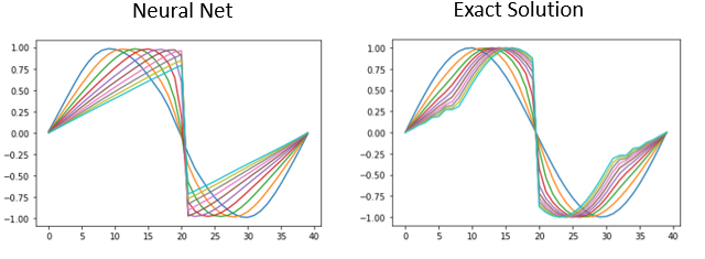
Figure 3.  The x axis x in the interval [-1,1] at 40 points and the y axis is u(t,x).  Each line represents u(t, x) for a specific value of t.   The blue line is the initial condition t=0.  Subsequent lines show the evolution to the singularity.

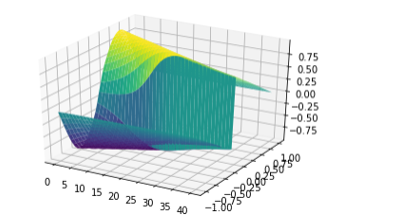
Figure 4.   A 3D view showing the evolution of the sine wave on the left to the sharp shock on the right edge.

Nonlinear Boundary Value Problems

The classical elliptical PDE takes the form

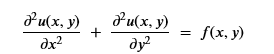
where u is defined on a region in x-y space and known on a bounding edge.   A good physical example is a steel plate that is clamped and temperature controlled on perimeter and f represents heat applied to the surface.  u will represent the temperature when it reaches a steady state.

For purposes of illustration we can consider the one-dimensional case, but to make it interesting we will add some non-linear features.  In addition to the function f(x),  let us add another known function k(x) and consider

To show that the technique works, we will consider special cases where we know the exact solution.  We will let k(x) = x and u(x) = sin²(x).    Taking the derivative and applying a few trig identities we get f(x) as

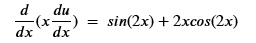
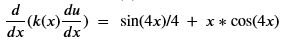
Where we will look for the solution u on the interval [0, pi] subject to the boundary condition u(0) = u(1) = 0.  The second case will be similar, but the solution is much more dynamic: u(x) = sin²(2x)/8 with the same boundary conditions.   In this case the operator is

The network is like the one above but with only one input parameter

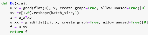
The differential operator that is the left side of the equation above is computed with the function Du(x) shown below.

Training the network is straightforward.  As with the Burgers example, we use a mean squared error lost function and gradient descent optimizer. We have an array vx of x-axis points from which batches of samples are drawn.   For each point x in each batch we also create a batch consisting of f(x).  There is only one batch for the boundary.   In this case, the boundary is only two points, so it is represented by one batch.

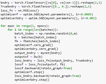
Running this for 3000 epochs with batch of size 10 will converge the network.   The result for the 1^st case (u = sin²(x) ) is extremely close to the exact solution as shown in figure 5.   Both the true solution (a blue line) and the computed solution (an orange line) are plotted together.   They are hard to distinguish.   Below the solution we plot the differential equation f(x) which is what the networked was trained to learn and it is not surprising the fit is good there too.

The second case (u = sin²(2x)/8 ) is more dynamic.    The differential equation f(x) fit is excellent but the solution is shifted up (because the boundary condition was off on one end.

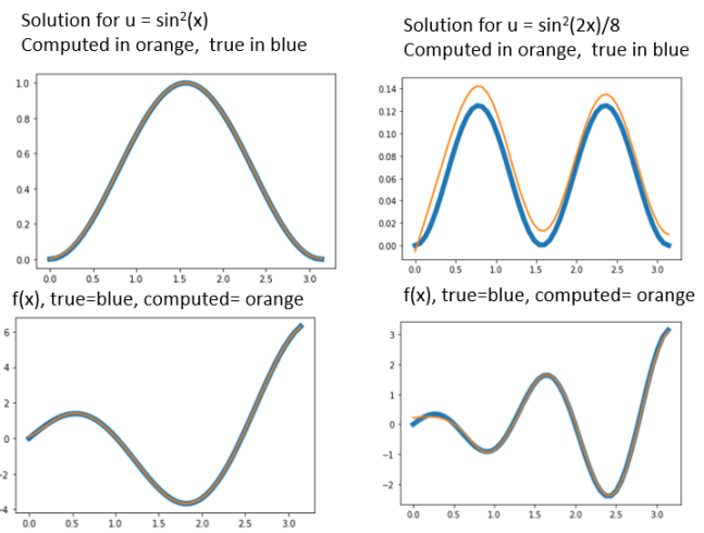
Figure 5.   Solution to the differential equation d/dx(x du/dx) = f(x)

Stochastic Differential Equations and Generative Adversarial Nets

If we consider the differential equation from the previous section

but now make the stipulation that the functions k(x) and f(x) are Gaussian processes rather than fixed functions, we now have a stochastic differential equation.   Papers 2 and 3 mentioned above show us how to create a generative adversarial network to solve for the Gaussian process that defines u.  they do not treat this as an initial value, boundary value problem as described above, but rather the authors assume we have a series of snapshots  ( k(x_i), u(x_i), f(x_i) ) for i in 1, … n for some reasonably large n.  With these we will set up a GAN to find a representation of u.

Recall how a GAN works.  We have two networks, a generator, and a discriminator.  The generator is trained to transform a normal distribution into a distribution that fits your data.  The discriminator is trained to recognize your true data and distinguish it from the fake data from the generator.  This is illustrated in Figure 6 below.

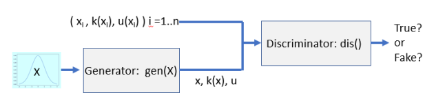
Figure 6.  Basic GAN configuration.

It is relatively easy to build a GAN that can reproduce u from samples of x, k(x) and u(x).  Unfortunately, making a GAN that looks like u(x) does not mean it satisfies the differential equation.  Taking the simple case where k(x)=x, a GAN base based on the design above generated the result in Figure 7 below.  On the left is a plot of the distribution of the converging solution for random normally distributed samples X over the true solution in blue (see right half of figure 5).  However, when we apply the differential operator to the generated solution we see it (multi-colored dots) is nothing like our the true solution operator (blue).

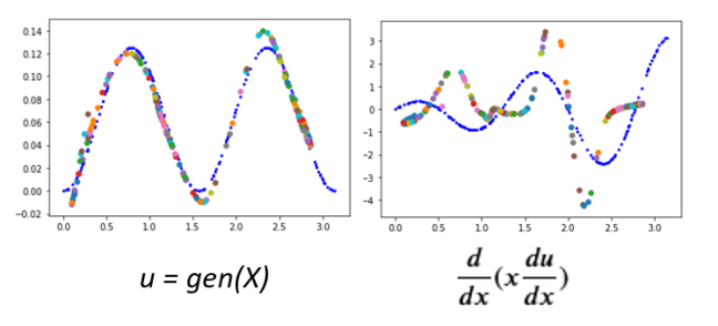
Figure 7.  GAN from figure 6 distribution of normally distributed sample X and, on right differential operator applied to gen(X)

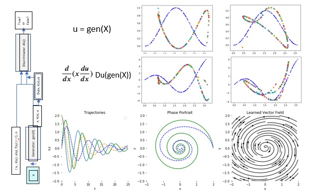
To solve this problem the GAN discriminator must evaluate both u(x) AND the result of the differential operator f(x) = Du(x, k(x), u) as show in Figure 8.

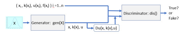
Figure 8.  Full GAN to map normal distribution to solution that also satisfies the differential equation.

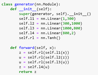
The construction of the GAN generator is straight forward.  It takes inputs as batches of samples from a normal distribution and generates a batch of points in R² that are eventually trained to represent samples from (x, u(x)).   As for our previous examples we use Tanh () for the activation function.

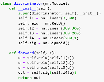
The discriminator takes triples of the form (x_i, u(x_i), f(x_i)) from the samples.  (Note we are using k(x)=x, so there is no need for that argument.   We can use ReLU for the activation because we do not need second derivatives of the discriminator.

The torch version of the differential operator is

The discriminator wants inputs of the form

Which are provided by the samples (x_i, u(x_i), f(x_i)) and from the generator in the form

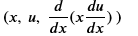
The training algorithm alternates between optimizing  log(D(G(z))) for the generator and optimizing log(D(x)) + log(1 – D(G(z))) + a gradient penalty for the discriminator.   The gradient penalty is introduced by Yang, Zhang, and Karniadakis in paper 2.  The full code for this example is in the Github repository.  Figure 9 illustrates the convergence of the solution in for snapshots (A, B, C, D) with step D taken at 200000 epochs.  It is interesting to observe that image of the 1-D normal sample space in R² takes to form of a path that gradually conforms to the desired distribution.  However at step D there is still unfocused resolution for x > 2.6.

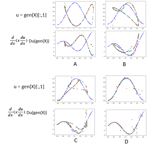
Figure 9.   Four snapshots in time (A, B, C, D) of the convergence of the GAN.

We should also note that this is not a true stochastic PDE because we have taken our samples for the training from the exact solution and are not Gaussian sources, but the concepts and training are correct.

A much more heroic and scientifically interesting example is in paper 3.   The authors of this paper address the problem of modeling the subsurface flow at the Hanford Site in Washington State where the reactors to generate plutonium for the US atomic arsenal.   The 500 square mile site had nine nuclear reactors and five large plutonium processing complexes and produced 3 million US gallons of high-level radioactive waste stored within 177 storage tanks, an additional 25 million cubic feet of solid radioactive waste.  And over the years the tanks have been leaking.   Hanford is now nation’s largest environmental cleanup project.   The team involved with paper 3 is from Brown University, Lawrence Berkeley National Lab, Pacific Northwest National Lab, Nvidia, Julia Computing and MIT.  They look at a large 2-D version of the PDE discussed above.   In this case u(x,y) is hydraulic head of the subsurface flow, k(x,y) is depth-averaged hydraulic conductivity and f is the infiltration from the earth to the flow.   These quantities are measured by sensors at a large number of sites on the Hanford reservation.

Because k and u are both stochastic and are supported only by data at the sensor points the generator in their GAN must produce both k and u (actually  log(k) and u) as shown in Figure 10.

Figure 10.  GAN architecture from Yang, et. al, “Highly-scalable, physics-informed GANs for learning solutions of stochastic PDEs”, arXiv:1910.13444v1.

In order to tackle a problem of the size of the Hanford problem, they partitioned the domain into a hierarchy of subdomains  and had a separate discriminator for each subdomain.   The top levels (1 and 2) capture long range characteristics while the lower levels capture properties that correspond to short range interactions.   They parallelized the computing utilizing over 2700 GPUs on the ORNL Summit machine so that it maintained 1.2 exaflops.

Neural Ordinary Differential Equations

In the previous section we saw how neural networks can solve differential equations.   In this section we look at the other side of this coin: how can differential equation solvers simplify the design, accuracy, and memory footprint of neural nets.   Good papers and blogs include the following.

1. Chen, Rubanova, Bettencourt, Duvenaud “Neural Ordinary Differential Equations”
2. Colyer, Neural Ordinary Differential Equations, in the Morning Paper, Jan 9, 2029, Colyer’s amazing blog about computer science research.
3. Duvenaud, comments in Hacker News about the Chen, et. al. paper.
4. Chen, “PyTorch Implementation of Differentiable ODE Solvers”.
5. Rackauckas, “Mixing Differential Equations and Machine Learning” .
6. He, et. al. “Deep Residual Learning for Image Recognition”.
7. Gibson, “Neural networks as Ordinary Differential Equations”
8. Holländer, “Paper Summary: Neural Ordinary Differential Equations”
9. Surtsukov, “Neural Ordinary Differential Equations”

Chen et. al. in [1] and others have observed that the deep residual networks that made training very deep networks possible [6] had a form that looked like Euler’s method for solving a differential equation.  Residual networks use blocks of network layers where the input is transformed by a residual before sending it to the next layer by the simple equation

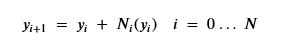
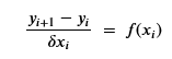
So that what we are training is the sequence or residual layers N_i  .  If you have a differential equation dy/dx = f(x) then Euler’s method is to compute y from a sequence of small steps of based on an approximation of dy/dx by

By analogy, our residual network now looks like this

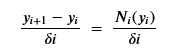
With delta i is equal to 1.   If we abstract the sequence of networks into a single network that depends upon t as well as y, we can define a neural ODE to be of the form

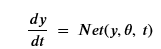
Where theta represents the network parameters.

The interesting idea here is that if residual networks are basically Euler’s method applied then why not use a much more modern and accurate differential equation solver?  If we have an initial value y₀ at  time t₀, we can integrate forward to time t_n to obtain

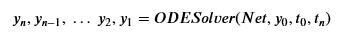
To illustrate how we can train a neural ordinary differential equation we look at a slightly modified version of the ode_demo.py example provided by the authors. we will take our sample data from the solution of a simple ODE that generates spirals in 2-D given by

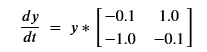
Where y is a 2-d row vector.   Given the starting point y₀ = (2.0, 0.0) and evolving this forward 1000 steps the values are plotted below.

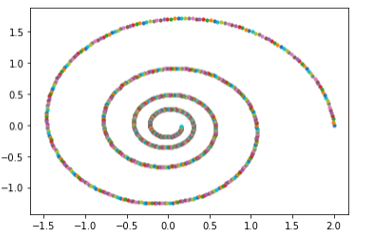
Figure 11.  Spiral Training Data

Our neural network is extremely simple.

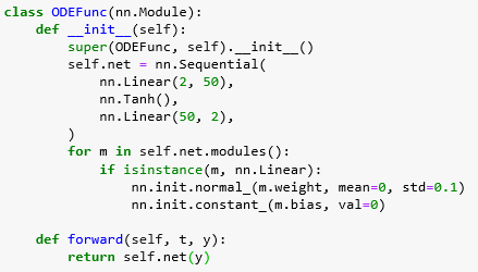
You will notice that while the network takes a tuple (t, y) as input, the value t is unused.  (This is not normally the case.) The training algorithm is quite simple.  Recall that the function is a derivative, so to predict new values we must integrate forward in time.

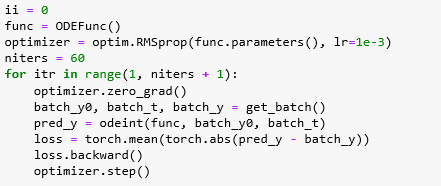
The authors use Hinton’s Root Mean Square Propagation optimizer. And the function get_batch() returns a batch of 20 points on the spiral as starting points as batch_y0.  Batch_t is always the 10 time points between 0 and 0.225 and batch_y is a batch of 20 10-step paths along the spiral starting from the corresponding batch_y0 point.   For example, shown below is a sample batch.

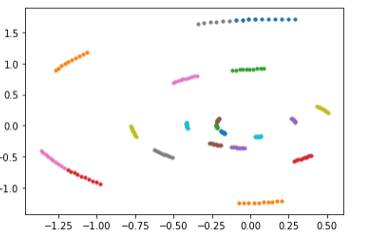
Figure 12.  Sample training data batch

An incredibly important point is a property of the ODE solver we use “odeint”.

It comes from the author’s  torchdiffeq package as an adjoint integrator.  The actual integrator we want to use is scipy.integrate.odeint which is a wrapper for an old, but sophisticated method written in the 1980s and from ODEPACK.  But we need to be able to compute the symbolic derivative of the loss operation so we can do the backpropagation.   But we can’t do the symbolic integration back through the old ODEPACK solver.  To get around this problem the Chen and the team uses the integrator to solve an adjoint problem which, very cleverly, allows us to compute all the derivatives without trying to differentiate the solver.  The details of this step are described in the original paper and in the other references above.  We won’t go into it here.

It is fun to see the result of the training as the it evolves.   We captured the output every 10 iterations.

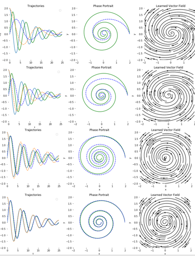
Figure 13.  Snapshots of training showing the trajectories of the solution and the correct values.

It is worth observing that, once trained our network, when given a point (x, y) in the plane returns a vector of the trajectory of the spiral path through that point.   In other words, it has learned a vector field which can be plotted as on the right in figure 13 and below.

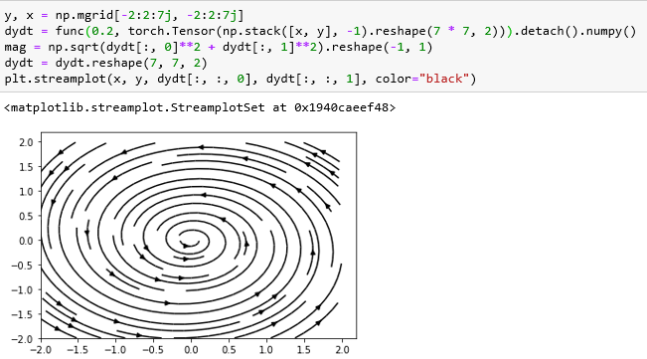
Figure 14.  plot of the vector field generated by the network

Neural ODEs can be applied well beyond applications that resemble simple differential equations.  The paper illustrates that they can be applied to the vision tasks that resnet was invented to solve.  The paper show how it can be applied to build a MNIST hand written digit classifier but with a much smaller memory footprint (one layer  versus many layers in resnet).  There is a very nice implementation in Surtsukov [9].

The solution (detailed in Surtsukov’s notebook in his gitub repo) also contains all the details of the solution to the adjoint problem for computing the gradients of the loss.   The model to classify the MNIST images is almost identical to the classical Resnet solution.   A slightly modified version that combines parts of Surtsukov’s solution with Chen’s solution  is in our Github repo.

The input to the model is passed through an initial down-sampling followed by the residual blocks that compute the sequence

More specifically the Resnet version consists

• A down sampling layer
• 6 copies of a residual block layer
• And a layer that does the final reduction to 10 scores.

The neural ODE  replaces the six residual layers N_i(y_i ) with the continuous derivative  N(y,t).  The forward method of the NeuralODE invokes the adjoint solution to the integration by using the odeint() function described in the previous example.   You can experiment with this in the Jupyter notebook in the repo.  With one epoch of training the accuracy on the test set was 98.6%.  Two epoch put it over 99%.

One of the other applications of Neural ODEs is to time series data.  A challenge for many tradition neural network approaches to time series data analysis is that they require uniformly spaced samples for training.  Because the Neural ODE is continuous,  the sampling can be flexible and adaptive.

Final Thoughts

This report is an attempt to illustrate a striking duality that seems to exist between deep neural networks and differential equations.   On the one hand, neural networks are non-linear functions that, with the right choice of activation functions, can have smooth first and second derivatives and, consequently, they can be trained to solve complex differential equations.    Generative adversarial networks can even model the solution to stochastic differential equations that fully satisfy the governing laws of physics.  Seen from another perspective, many deep networks are just discrete approximations to continuous operators that can be solved with advanced differential equations packages.   These Neural ODEs have much smaller memory requirements and are more adaptive in their execution and may more accurately solve difficult problems.

It is going to be interesting to see where these approaches lead in the years ahead.

The github repository for this paper contains four Jupyter notebooks:  the solution to Burger’s equation, the simple non-linear and generative adversarial example, and the simple Neural ODE solution to the spiral described above and the MNIST solver.

Postscript. I realize now that I overlooked another significant contribution to this discussion.  “Deep Learning Based Integrators for Solving Newton’s Equations with Large Timesteps” arXiv:2004.06493v2 by Geoffrey Fox and colleagues show how RNN can be use to vastly improve the performance of the integration of Newton’s equation.