
In this tutorial, we are going to cover the basics of Tensors in TensorFlow.
This blog post is the first in the series Getting Started with TensorFlow.
- Introduction to Tensors in TensorFlow.
It’s been a while since TensorFlow 2.x (2.0, 2.1, 2.2, and so on) came out. And it brings many new features and improvements with it. The best way to know about all these improvements and features is to get familiar with the basics.
Covering the important parts of any machine learning or deep learning framework/library by breaking them down to the basics, makes it really easy when writing complex models and code. This is what we aim to achieve with this Getting Started with TensorFlow series. We will cover a small topic with each part of the series. This will make things much clearer than if we directly jump into the advanced deep learning stuff. And don’t worry, we will cover training tutorials in this series as well.
So, what are we going to cover in this tutorial?
- Installing TensorFlow 2.x locally.
- Creating different rank tensors (Rank 0, Rank 1, Rank 2, Rank 3).
- Specifying data types while creating tensors.
- Converting tensors to NumPy arrays.
- Converting NumPy arrays back to tensors.
- Basic arithmetic operations in tensors.
- Interoperatbility Between Tensors in TensorFlow and NumPy Arrays.
- GPU acceleration for TensorFlow tensors.
- How to specify CPU and GPU operations manualy?
I hope that you are excited to follow along till end the end of the tutorial. Let’s start with the installation of TensorFlow.
Installing TensorFlow 2.x
Starting from TensorFlow 2.x, installation on local machines is a breeze. The only thing you need, either a Python virtual environment or a Conda environment.
Step 1: Create a Separate Environment
It is always better to install any new versions of a deep learning framework or library in a separate environment. You can choose to create either a Python virtual environment or a Conda environment, whichever you prefer. We will not go into the details of creating one here. If you are absolutely new to this, then you can follow this post which provides a concise, yet complete procedure for the same.
Step 2: Install TensorFlow
After you create your virtual environment and activate it, install TensorFlow using the following command.
pip install tensorflow
This installs the latest stable version of TensorFlow for both, CPU and GPU. At the time of writing this series, TensorFlow 2.5 is the latest stable version. So, all the tutorials in this series will use TensorFlow 2.5.
Step 3: Check the TensorFlow Version
The final step is to check whether TensorFlow is installed correctly and its version.
Open your terminal, activate your TensorFlow environment, and type python to enter the Python CLI.
Then type the following commands.
>>> import tensorflow as tf
2021-07-10 07:00:54.696570: I tensorflow/stream_executor/platform/default/dso_loader.cc:53] Successfully opened dynamic library libcudart.so.11.0
>>> print(tf.__version__)
2.5.0
First, we import TensorFlow and check the TensorFlow version. You can see that the version is 2.5.0, which we will use throughout the series.
One other good thing starting from the installation of TensorFlow 2.x is that it installs both, the CPU and GPU compatible packages. This means that we do not need to install any GPU-specific things separately. And if you have an NVidia GPU in your system with CUDA and cuDNN already set up, then you are good to go to benefit from the GPU accelerated tensor operations.
Now, that we are done with installing TensorFlow, let’s start to learn about tensors in TensorFlow with a more hands-on approach.
Note: All the code in this tutorial is expected to be run on Jupyter Notebook. Although you can always opt for Python scripts, it is easier to follow along with a notebook for this tutorial.
Tensors in TensorFlow
Before getting into the hands-on part, let’s try to answer one simple question in short. What are Tensors in deep learning?
Generally, we define tensors as multidimensional arrays on which we can perform basic mathematical operations like multiplication and addition easily.
But with the current deep learning frameworks, sometimes, tensors may not be multidimensional. They can be single numbers which we will see just a bit further on.
Tensors with Different Ranks
In this section, we will see tensors with different ranks, namely, rank 0, rank 1, rank 2, and rank 3 tensors.
Sometimes, getting familiar with the ranks of tensors gets beginners confused who are just starting out with deep learning. So, let’s try to simplify them as much as possible.
First, we need to import tensorflow and numpy as these are the two packages that we will use throughout this tutorial.
import tensorflow as tf
import numpy
import numpy as np
Rank-0 Tensor
We can call a rank-0 tensor a scalar as well. This is just a single value without any axes or even a shape.
Take a look at the following code block.
rank_0 = tf.constant(10)
print(rank_0)
print(rank_0.shape)
The first thing to note in the above block is that we are using tf.constant() to create a tensor. Be it a rank-0 tensor or a rank-3 tensor, we always use tf.constant() to create tensors in TensorFlow. Then we are printing the tensor itself and its shape.
The following block shows the output.
tf.Tensor(10, shape=(), dtype=int32)
()
A few things to note here:
- The tensor value is 10. And it is a
Tensor()object which is represented bytf.Tensor(). - The shape of the tensor is
(), that is, empty. This is because it is a single number, or a scalar, or a tensor with no axes. You can choose to call it whatever you prefer. - Finally, it also has a
dtype(data type). It isint32by default, which is understandable given we passed the number 10 to thetf.constant()function.
Coming to the dtype once again. What will be the default dtype if we provide a floating-point value to the function? Well, let’s check it out.
# a floating point number
rank_0 = tf.constant(10.)
print(rank_0)
print(rank_0.shape)
tf.Tensor(10.0, shape=(), dtype=float32)
()
You see, this time, the dtype is float32 by default. So, we can conclude that the tf.constant() function can infer the data type of the number we are passing and assign it accordingly.
Rank-1 Tensor
A rank-1 tensor is also called a vector. Unlike the rank-0 tensor, it does have one axis and even a shape.
rank_1 = tf.constant([1, 2, 3])
print(rank_1)
tf.Tensor([1 2 3], shape=(3,), dtype=int32)
If you observe closely, you will conclude a few things.
- First, a rank-1 tensor is a list of values, if seen with the Python language paradigm.
- But unlike a Python list, it does have a shape. Which is
(3, )in this case. This is just like a NumPy array containing three numbers. - And the dtype is again
int32by default.
From the above points, we can sense that tensors in TensorFlow have some relationship with NumPy arrays. In one of the further sections, we will see how to convert tensors to NumPy arrays and vice-versa.
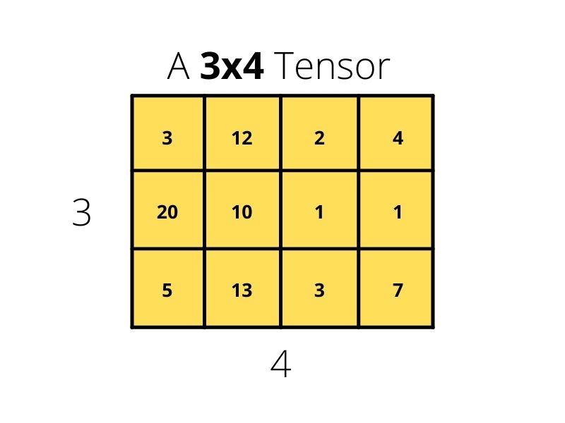
Rank-2 Tensor
A rank-2 tensor is very similar to a matrix or a 2D NumPy array. It has two axes as well.
rank_2 = tf.constant([
    [10, 12],
    [20, 22],
    [30, 32],
])
print(rank_2)
tf.Tensor(
[[10 12]
 [20 22]
 [30 32]], shape=(3, 2), dtype=int32)
- We can see that the tensor has 2 axes.
- The shape is
(3, 2)with default data type ofint32.
This was pretty easy. Let’s move on to rank-3 tensors.
Rank-3 Tensor
A rank-3 tensor has 3 axes and is similar to a 3D Numpy array.
rank_3 = tf.constant([
    [
        [1, 2, 3, 4],
        [5, 6, 7, 8],
    ],
    [
        [9, 10, 11, 12],
        [13, 14, 15, 16],
    ],
    [
        [17, 18, 19, 20],
        [21, 22, 23, 24],
    ]
])
print(rank_3)
tf.Tensor(
[[[ 1  2  3  4]
  [ 5  6  7  8]]

 [[ 9 10 11 12]
  [13 14 15 16]]

 [[17 18 19 20]
  [21 22 23 24]]], shape=(3, 2, 4), dtype=int32)
The shape of the rank-3 tensor is (3, 2, 4). And by now you must have figured out that it looks very similar to a 3D NumPy array.
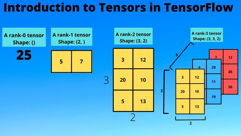
After rank-3, visualization of tensors can become very tricky. We will not dive into that for now. Nor is it required for the things that will come further on. For now, let’s visualize all the tensor images together so that the things that we have covered till now becomes even more clear.
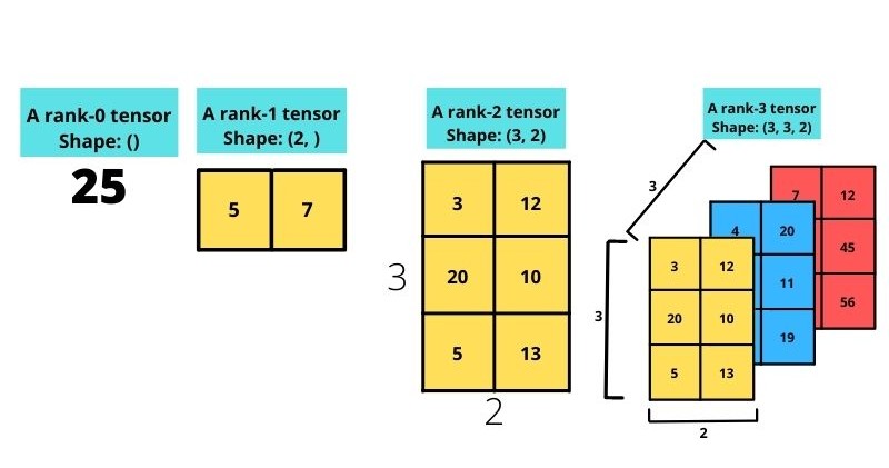
Figure 7 shows tensors from rank 0 till rank 3 and how their corresponding axes and shape keep changing throughout.
Changing Data Types of Tensors in TensorFlow
By default, tensors in TensorFlow will be assigned the data type according to the value we provide.
For example, if we provide an integer value to tf.constant(), then the default data type will be int32.
# default data type is int32
test_tensor = tf.constant(1)
print(test_tensor)
tf.Tensor(1, shape=(), dtype=int32)
But when we provide a floating-point value to tf.constant(), then the default data type will be float32. Let’s confirm that with some basic code.
# default data type is float32
test_tensor = tf.constant(1.)
print(test_tensor)
tf.Tensor(1.0, shape=(), dtype=float32)
By now, we know that the data type depends on the value we provide. But what if we want to explicitly define the data type while creating the tensor? We can do that too!
Let’s create a tensor of having data type float32.
# define a float32 value
test_tensor = tf.constant(1, dtype=tf.float32)
print(test_tensor)
tf.Tensor(1.0, shape=(), dtype=float32)
For one final test, let’s create a rank 2 tensor with data type float16.
# data type float16
test_tensor = tf.constant([1, 2], dtype=tf.float16)
print(test_tensor)
tf.Tensor([1. 2.], shape=(2,), dtype=float16)
In the above rank 1 tensor, all the elements will have a float16 data type. We can easily confirm that also by checking the individual data types as there are only two elements.
print(test_tensor[0].dtype)
print(test_tensor[1].dtype)
<dtype: 'float16'>
<dtype: 'float16'>
Now, it is pretty clear how we can assign the data types while creating tensors in TensorFlow.
Converting TensorFlow Tensors to NumPy Arrays
Now, let’s check out how we can convert the TensorFlow tensors to NumPy arrays. This is also pretty easy.
We will create a rank 1 tensor and convert that to a NumPy array.
test_tensor = tf.constant([23, 24])
# convert the tensor to NumPy array
test_numpy_1 = np.array(test_tensor)
print(test_numpy_1, type(test_numpy_1))

# OR
test_numpy_2 = test_tensor.numpy()
print(test_numpy_2, type(test_numpy_2))
[23 24] <class 'numpy.ndarray'>
[23 24] <class 'numpy.ndarray'>
We can choose either of the two ways to convert the tensors to NumPy arrays:
- Either use the
array()method from NumPy while passing the tensor as the argument. - Or use the
Tensor.numpy()function to do so.
Both of the above methods will produce the same results as you can see.
NumPy Indexing
After the NumPy conversion, you can also apply the usual NumPy array indexing to the results.
Let’s check that out with a new example.
test_tensor = tf.constant([
    [1, 2, 3],
    [4, 5, 6],
    [7, 8, 9]
])

test_numpy_3 = test_tensor.numpy()
# print 0th element of all the rows
print(test_numpy_3[:, 0])
[1 4 7]
First, we create a rank 2 tensor. Then we convert the tensor to NumPy array. This allows us to apply the usual NumPy indexing that we are all familiar with and we are printing the 0th element of all the rows in the new NumPy array.
Converting NumPy Arrays Back to TensorFlow Tensors
In the above code block, we converted the tensor test_tensor to a NumPy array, test_numpy_3.
Can we convert the NumPy array back to tensor? Yes, we can. TensorFlow provides the convert_to_tensor() function to convert any NumPy array to tensor format. The following code block provides an example for the same.
test_tensor_new = tf.convert_to_tensor(test_numpy_3)
print(test_tensor)
tf.Tensor(
[[1 2 3]
 [4 5 6]
 [7 8 9]], shape=(3, 3), dtype=int32)
We can see that the NumPy array has been converted to a TensorFlow Tensor() object after passing the test_numpy_3 array as an argument to the convert_to_tensor() function. The result is stored in a new tensor variable called test_tensor.
Basic Arithmetic Operations with Tensors
Here, we will look at a few of the arithmetic operations that we can carry out with tensors.
Tensor Addition
As the name suggests, this is the addition of two tensors. TensorFlow provides the add() function using which we can add two tensors.
Let’s create two rank 0 tensors and add them.
tensor_1 = tf.constant(1)
tensor_2 = tf.constant(2)

print(tf.add(tensor_1, tensor_2))
tf.Tensor(3, shape=(), dtype=int32)
As expected, the is a tensor with a value of 3 having int32 data type.
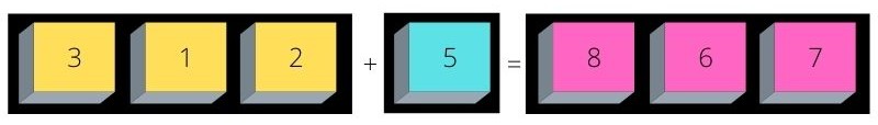
Now, let’s try adding a rank 0 tensor with a rank 1 tensor.
tensor_3 = tf.constant([3, 4, 5])
print(tf.add(tensor_1, tensor_3))
tf.Tensor([4 5 6], shape=(3,), dtype=int32)
In this case, the rank 0 tensor, i.e., 1, is added to each element of the rank 1 tensor. This results in a new rank 1 tensor.
Tensor Multiplication
Moving on to tensor multiplication in TensorFlow. We can carry out tensor multiplication using TensorFlow’s multiply() function. This returns an element-wise multiplication between two tensors.
Let’s check out a simple example.
tensor_4 = tf.constant([1, 2, 3])
tensor_5 = tf.constant([4, 5, 6])
print(tf.multiply(tensor_4, tensor_5))
We have two rank 1 tensors called tensor_4 and tensor_5 which we multiply using tf.mulitply(). The following is the result.
tf.Tensor([ 4 10 18], shape=(3,), dtype=int32)
We have a rank 1 tensor as the result and each of the values in the tensor is an element-wise product of the above tensor_4 and tensor_5.
Interoperability Between Tensors and NumPy Arrays
Tensors in TensorFlow and NumPy arrays can interoperate. This means that we can carry out basic arithmetic operations between the tensors and NumPy arrays directly even if they are not of the same type.
The following code block shows a simple example.
tensor_1 = tf.constant(1)
numpy_1 = np.array(2)

result_1 = tf.add(tensor_1, numpy_1)
print(result_1)
result_2 = tf.multiply(tensor_1, numpy_1)
print(result_2)
tensor_1 is a tensor and numpy_1 is a NumPy array. Still, we can use TensorFlow’s add() and multiply() functions on them to obtain the results.
tf.Tensor(3, shape=(), dtype=int32)
tf.Tensor(2, shape=(), dtype=int32)
And the final result will be converted to a TensorFlow Tensor() object automatically.
GPU Acceleration for Tensors
One great thing about tensors in deep learning. We can use the power of a GPU (Graphics Processing Unit) to accelerate the basic arithmetic as well as deep learning specific operations. And if you have CUDA and cuDNN already set up in your system, then TensorFlow automatically uses GPU for all the arithmetic operations.
We can start by checking the availability of GPU in our local system.
# check GPU availability
print(f"Devices available: {tf.config.list_physical_devices()}")
The above code lists all the computation devices available.
If you have an NVidia GPU in your system, then you should get the following output.
Devices available: [PhysicalDevice(name='/physical_device:CPU:0', device_type='CPU'), PhysicalDevice(name='/physical_device:GPU:0', device_type='GPU')]
The above output shows that the system has a CPU as well as a GPU to carry out the computations.
Let’s initialize a tensor and check whether it is being loaded onto the GPU or not.
# check of the tensor is on CPU or GPU
test_tensor = tf.constant(3)
print(test_tensor.device)
print(test_tensor.device.endswith('GPU:0'))
/job:localhost/replica:0/task:0/device:CPU:0
False
We can see that the tensor is on the CPU. Until and unless we carry out any operation using this tensor, it will not be loaded onto the GPU by default.
To check that, we will initialize two tensors and apply the add() and multiply() operations on them.
# Create some tensors
a = tf.constant([
    [1, 2, 3],
    [4, 5, 6],
])
b = tf.constant([
    [7, 8, 9],
    [10, 11, 12],
])

print(a.device)
print(b.device)

c = tf.add(a, b)
print(c)
print(c.device)

d = tf.multiply(a, b)
print(d)
print(d.device)
We are operating on two rank 2 tensors, a and b. The addition and multiplication results are stored in tensors c and d respectively. Let’s check out the results.
/job:localhost/replica:0/task:0/device:CPU:0
/job:localhost/replica:0/task:0/device:CPU:0

tf.Tensor(
[[ 8 10 12]
 [14 16 18]], shape=(2, 3), dtype=int32)
/job:localhost/replica:0/task:0/device:GPU:0

tf.Tensor(
[[ 7 16 27]
 [40 55 72]], shape=(2, 3), dtype=int32)
/job:localhost/replica:0/task:0/device:GPU:0
First, tensors a and b are on the CPU at the time of initialization. Tensor c, after the addition, is on the GPU, and the same goes for tensor d after the element-wise multiplication.
Matrix Multiplication on the GPU
By now you must have noticed that we have carried out element-wise multiplication on two tensors. But what about matrix multiplication?
Here, we will see how to carry out matrix multiplication on two tensors using the GPU. Let’s check out the following code block.
# 3x2 tensor
d = tf.constant([
    [1.0, 2.0],
    [3.0, 4.0],
    [5.0, 6.0],
])
# 2x2 tensor
e = tf.constant([
    [7.0, 8.0],
    [9.0, 10.0]
])

f = tf.matmul(d, e)

print(f)
print(f.device)
First, we create a tensor d which is a 3×2 tensor. Tensor e is a 2×2 tensor. Note that the number of columns of the first matrix should be the same as the number of rows in the second matrix for the matrix multiplication to take place correctly. This is the typical matrix multiplication constraint that we have in mathematics as well.
Secondly, we use the tf.matmul() function to carry out the matrix multiplication using the above two tensors. The following is the result.
tf.Tensor(
[[ 25.  28.]
 [ 57.  64.]
 [ 89. 100.]], shape=(3, 2), dtype=float32)
/job:localhost/replica:0/task:0/device:GPU:0
As expected, the result is a 3×2 matrix with float32 data type. And we can see that the operation took place on the GPU and therefore, the result is also stored in the GPU.
Specifically Using the CPU
There might be scenarios where we want the operation to take place on the CPU. Maybe we know beforehand that the operation is not compute-intensive and a CPU can handle it pretty easily. In such cases, we need to specify the computation device.
We can do so using the tf.device() function. The following block shows one example.
with tf.device('/CPU:0'):
    # 3x2 tensor
    d = tf.constant([
        [1.0, 2.0],
        [3.0, 4.0],
        [5.0, 6.0],
    ])
    # 2x2 tensor
    e = tf.constant([
        [7.0, 8.0],
        [9.0, 10.0]
    ])

    f = tf.matmul(d, e)

print(f)
print(f.device)
We use the with tf.device('/CPU:0') to initialize the tensors and carry out the matrix multiplication as well. Let’s check out the results.
tf.Tensor(
[[ 25.  28.]
 [ 57.  64.]
 [ 89. 100.]], shape=(3, 2), dtype=float32)
/job:localhost/replica:0/task:0/device:CPU:0
As the operation used the CPU instead of the GPU, so, the resulting tensor f is also attached to the CPU.
Summary and Conclusion
In this tutorial, you learned about the basics of tensors in TensorFlow. We started with learning about the different ranks of tensors. Then we saw how to specify the data type while creating tensors. Then we moved on to converting tensors to NumPy arrays and vice-versa. After that, we carried out some basic arithmetic operations using the tensor. Finally, we checked out how to specifically use the GPU and CPU for operating on tensors. I hope that you learned something new in this tutorial.
If you have any doubts, thoughts, or suggestions, then please leave them in the comment section. I will surely address them.
You can contact me using the Contact section. You can also find me on LinkedIn, and Twitter.

7 thoughts on “Introduction to Tensors in TensorFlow”