Hierarchical logistic regression giving non-sensible results? Do I formulate it correctly?

[mrzeliboba]

Hello PyMC3 community, it would be really great to get your evaluation of my PyMC3 formulation of the simple hiearchical model. Somehow even on the synthetic data, the results are weird and there are two possible options for it: either I do something wrong in the PyMC modeling or the problem by itself is not well formulated for an approach chosen.

Formulation of the model:
Participant j \in [1 \dots N] completes the task i \in [1 \dots T] by choosing one of the two provided options (ways of completing the task) a_{ji} and b_{ji}. Each option a_{ji} and b_{ji} can characterized by two components:

a_{ji} = a^{\circ}_{ji} + a^{\bullet}_{ji}

We assume that components a^{\circ}_{ji} and a^{\bullet}_{ji} are not identical in the cost percieved by participant. We model the difference in cost of options:

\begin{align} \Delta c_{ji} &= \beta_j \Delta c^{\circ}_{ji} + \Delta c^{\bullet}_{ji} \\ &= \beta_j (a^{\circ}_{ji} - b^{\circ}_{ji}) + (a^{\bullet}_{ji} - b^{\bullet}_{ji}) \end{align}

The ultimate goal of the analysis is to estimate \beta_j — participant-specific inflation coefficient of component \circ as compared to component \bullet of costs associated with completing the tasks.

We model the choices in a probabilistic way. Probability of choosing option a_{ji} at choice i by participant j:

p(y_{ji}=1) = \frac{1}{1+\exp[\Delta c_{ji}/\tau_j]}

Where y_{ij} is indicator variable of whether option a_{ji} was chosen, \tau_j is a temperature parameter individual parameter for each participant, reflecting the sensitivity of participant’s decisions to the difference in the option’s costs.
In this model we assume that no learning is involved, the parameters are static during the experiment and that the decisions made by participant are independent one from another. Thus, likelihood of observing the decisions y_{j} = \{y_{ji}, \dots, y_{jT}\}:

p(y_{j}) = \prod^{T}_{i=1} p(y_{ji}=1) = \prod^{T}_{i=1}\frac{1}{1+\exp[\Delta c_{ji}/\tau_j]}

The hiearchical model can be expressed by diagram:

The PyMC3 model formulation looks as follows:

def pymc_hier_model(choices, a_components, b_components, participants, cauchy_param=5.):
""" Build the PyMC3 hiearchical model of choices.

Args:
    choices (np.array(N*T)): Array of indicators of whether option A was chosen by participant.
    a_components (np.array(N*T, 2)): Array of components characterizing option A.
        First column is circle component, second column is bullet component.
    b_components (np.array(N*T, 2)): Array of components characterizing option B.
        Analogous to previous param.
    participants: (np.array(N*T)): Array of identifiers of participant, who made a particular choice.
        Each element is in [0 ... N-1].
    cauchy_param (float): Parameter of hyperprior Half-Cauchy distribution.

Returns:
    pm.Model: Hiearchical model of the choices.
"""

participants_n = participants.max() + 1
with pm.Model() as model:
    # a_beta, b_beta, a_tau, b_tau
    hyperparams = pm.HalfCauchy('hyperparams', cauchy_param, shape=4)

    beta = pm.Gamma('beta', hyperparams[0], hyperparams[1], shape=participants_n)
    tau = pm.Gamma('tau', hyperparams[2], hyperparams[3], shape=participants_n)

    delta_c = beta[participants] * (a_components[:, 0] - b_components[:, 0]) \
            + (a_components[:, 1] - b_components[:, 1])

    p_dec = pm.Deterministic('p_dec', pm.invlogit(-delta_c / tau[participants]))

    decisions = pm.Bernoulli('decisions', p_dec, observed=choices)

return model

The questions would be:

• Does the formulation look OK?
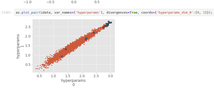
• If yes, why could that be that I get on the data generated with assumed data-generating process estimates of parameters (means), which no way look like accurate:
  
  

Thank you in advance!

[twiecki]

Have you tried using Normal/HalfNormal distributions rather than HalfCauchy and Gamma’s? Often these are easier to reason about. I would then do a prior predictive check first to see what types of data the model generates and tweak the priors to give you the rough results you expect to see.

[mrzeliboba]

Dear Thomas,

Thank you for your response. Yes, indeed, I found that model is super sensitive to priors, which is unexpected for a beginner, coz I set them super weakly informative. I have tried several ways to improve the results, including the reparameterization and different priors.

So far, the most reasonable results I could get are with the following reparameterization, estimation of transformed parameters and returning to original ones after sampling:

a_{ji} - b_{ji} = \Delta c^{\circ}_{ji} + \Delta c^{\bullet}_{ji} \\ \Delta c^{\bullet}_{ji} = (a_{ji} - b_{ji}) - \Delta c^{\circ}_{ji} \\ \begin{align} \Delta c_{ji} &= \beta_j \Delta c^{\circ}_{ji} + \Delta c^{\bullet}_{ji} \\ &= \beta_j \Delta c^{\circ}_{ji} + (a_{ji} - b_{ji}) - \Delta c^{\circ}_{ji} \\ &= (\beta_j - 1)\Delta c^{\circ}_{ji} + (a_{ji} - b_{ji}) \end{align}\\ p(y_{ji}=1) = \frac{1}{1+\exp[\Delta c_{ji}/\tau_j]}\\

\begin{align} \frac{\Delta c_{ji}}{\tau_j} &= \frac{(\beta_j - 1)\Delta c^{\circ}_{ji} + (a_{ji} - b_{ji})}{\tau_j} \\ &= \tilde{\beta_j}\Delta c^{\circ}_{ji} + \tilde{\tau_j}(a_{ji} - b_{ji}) \text{, where} \end{align} \\ \tilde{\tau_j} = 1 / {\tau_j} \sim \text{Inv-Gamma} \\ \tilde{\beta_j} = (\beta_j - 1)/{\tau_j} \sim \text{Normal}

Model diagram then looks like that:

Yet, I am far from convergence (there is always a message of \hat{R} > 1.05 (or even 1.4) with Metropolis step and 50K steps + 5K tuning steps. This does not seem OK, right?

I have also tried NUTS step, apart from being super slow (10 draw/s with NUTS vs 1.2K with Metropolis), after 1K samples it appears that it did not even explore much, all the \tau_j and \beta_j are around 1 or so.

• Would you say that using Half-Normal for p(\sigma) is appropriate? It has support at 0 which will drive things nuts, no? That is why I stick to Half-Cauchy. Or would you just add to it a small number to tackle this?
• Using direct parameterization and Log-normal/Normal priors resulted in all the samples stuck at one point – no exploration of sample space again.

Overall, I continue my exploration of probabilistic modeling with PyMC, looks like it is a lot about experience and intuition. Any advice is super appreciated. I also have notebook, in case you are so kind to have a closer look.

Thank you once again!

[nkaimcaudle]

Do you have a link to the notebook or code with example data we can look at?

[mrzeliboba]

Dear Nicholas, yes, I have tried to make it as clean and neat as possible. It would be great if you could have a look at it.

[nkaimcaudle]

Thanks, that is pretty complicated but well worked and with good graphics.

I didn’t look into the actual model very much but I could get it to run ok after some modifications.

• Standardise the a and b components
• Use NUTS
• Set a high target_accept
• Set a high number of tuning steps

After these I could get rhat around 1.04 (still on the high size, you want <1.01 ideally, and ess 160 with 1000 draws and 4 chains. But you could play around with the priors a lot more I reckon.

Standardise:
You’ll probably want to do this more elegantly but I just did it here. PyMC3 (and in general all probabilistic programming languages) prefer to have numbers not too high and not too low, Especially if you have a exponential or sigmoid somewere.

NUTS:
Metropolis is pretty universally discouraged, NUTS although more complex comes with the great benefit that if it complains then it nearly always means something is wrong in the model. Metropolis will just go along without warnings and you have no idea. In relation to speed, Metropolis may look faster initially but the ess/second is usually worse.

To get no divergences I used
trace = pm.sample(tune=5000, target_accept=0.99)
you could use more draws and tuning steps as you see fit.

[mrzeliboba]

Thank you, Nicholas. Could you share your figures of estimated parameters after you run it for 1000 draws with NUTS?

That is absolutely true, that the scale of the options is high. Standardising distorts original picture a bit, but just downscaling all options by a factor 100 (so that all \Delta c_{ji} \in [-1.5, 1.5] could be another to handle it.

Running the model with your advice to standardise and pm.sample(tune=5000, target_accept=0.99) gave no divergencies also and message of some parameters’ \hat{R} > 1.05, which is already good. But the estimates do not converge to true parameters, which is worrying. There is no even this approximate alignment along x=y line in scatters of true vs. estimated parameter (below). Did it look better in your case?

With other formulations, rescaling result in occurence of divergences. Adding more data per participant leads to expected drop in NUTS speed. Would you say, that thinking of different priors could improve things, or the whole model and it’s parameterization should be rethought?

Also, would you say, that Michael Betancourt’s “Conceptual intro in to HMC” is a good start to understand divergencies, ESS and overall NUTS, or there are more beginner-friendly resources?

Thank you once again.

[nkaimcaudle]

Seems that the model is over parameterised. You can see the first two and last two elements of hyperparams have correlation around 1.

Also it’s best to use non-centered parameterisations.

participants_n = participants.max() + 1
with pm.Model() as model:
    # a_beta, b_beta, a_tau, b_tau
    #hyperparams = pm.HalfCauchy('hyperparams', cauchy_param, shape=4)
    #hyperparams = pm.Normal('hyperparams', 0, 1, shape=2)
    locs = pm.Normal('locs', 0, 1, shape=2)
    scales = pm.HalfNormal('scales', 1, shape=2)

    #beta = pm.Gamma('beta', hyperparams[0], hyperparams[1], shape=participants_n)
    #beta = pm.Gamma('beta', tt.exp(hyperparams[0]), 1., shape=participants_n)
    #beta = pm.HalfNormal('beta', 5, shape=participants_n)
    beta_raw = pm.Normal('beta_raw', 0, 1, shape=participants_n)
    beta = pm.Deterministic('beta', tt.exp(locs[0] + scales[0]*beta_raw))
    #tau = pm.Gamma('tau', hyperparams[2], hyperparams[3], shape=participants_n)
    #tau = pm.Gamma('tau', tt.exp(hyperparams[1]), 1., shape=participants_n)
    #tau = pm.HalfNormal('tau', 5, shape=participants_n)
    tau_raw = pm.Normal('tau_raw', 0, 1, shape=participants_n)
    tau = pm.Deterministic('tau', tt.exp(locs[1] + scales[1]*tau_raw))
    
    #chol, corr, stds = pm.LKJCholeskyCov('lkj', eta=2., n=2, compute_corr=True, sd_dist=pm.HalfNormal.dist(1.))
    #params = pm.MvNormal('params', mu=0., chol=chol, shape=(participants_n, 2))
    #beta = pm.Deterministic('beta', tt.exp(params[:, 0]))
    #tau = pm.Deterministic('tau', tt.exp(params[:, 1]))

    delta_c = beta[participants] * (a_components[:, 0] - b_components[:, 0]) \
            + (a_components[:, 1] - b_components[:, 1])

    p_dec = pm.Deterministic('p_dec', pm.invlogit(-delta_c / tau[participants]))
    #p_dec = pm.Deterministic('p_dec', pm.invlogit(-delta_c / tau))

    decisions = pm.Bernoulli('decisions', p_dec, observed=choices)

return model

This runs fast and gives ok convergence, max rhat<1.01 and min ess>800. The posterior is still not great at recovering the true parameters. They are within the 94% hdi though,
np.logical_and(az.hdi(betas[None, ...])[:, 0] < participant_beta, participant_beta < az.hdi(betas[None, ...])[:, 1]).mean()
equals 1.00

I also played around with a 2d multi-variate normal, as you can see in the commented out code, it runs and gives ok results but takes over 10 times as long to run (15mins versus 1min).

@AlexAndorra is the maestro at web resources and learning. The pdf you link to is pretty heavy on the maths side, there should be some other links that give a higher level intro. Here is an 1hr long youtube video that introduces MCMC. The entire playlist is decent if you have time to go over it.

[AlexAndorra]

Indeed, all your hyper parameters are very correlated:

• More informative priors could help
• Reparametrizing with a non-centered version, as @nkaimcaudle did, should help too
• At worst, the data you have don’t have enough information about the parameters you’re trying to infer, so you might have to lower your expectations

The paper you linked too is very good, but very math-heavy so I clearly wouldn’t recommend it to beginners. The link Nicholas’ shared is great, as well as the accompanying book, Statistical Rethinking 2. Bayesian Analysis with Python, by Osvaldo Martin (a PyMC dev), is also a very good resource to get started. You can find more here.
To cite some of Betancourt’s work, this article is a good start to understand divergences a bit better, and I like this one about choice of priors!

Hope this helps
PS: Nicholas is too kind calling me a maestro

[mrzeliboba]

Wow, Richard McElreath, definetely has a style. Super nice lecture! Thank you guys for advice, I have got some few things to check on now.
This correlation between hyperparameters 0 and 1, and 2 and 3 is understandable as they are a and b of Gamma distribution, so to preserve lets say mean, increasing one of them would imply increasing another. There is also hyperbolic relation between hyperparams 0/1 and 2/3 because they are regulating distributions of two variables which are divided one by another in the model. So, I will try, to fix, say, a of Gamma distributions and make one b being estimated through hiearchical model.
Will also integrate non-centered version of the model parameterization.

[mrzeliboba]

Great resources, thank you! I now start with simpler formulation with estimating only \beta_j per subject and pooling \tau for all of them. Otherwise it indeed can be too optimistic to get that complex model to give reasonable estimates on the data I have.

Thank you once again, and I will post my results soon.

[nkaimcaudle]

Good news. Indeed it is often better to start with a simpler model, then you can add some complexity and see if it brings any benefit.

By the way, one technique for dealing with two highly correlated parameters is to rather than do:
a ~ N(0, 1)
b ~ N(0, 1)
c = aa_data + bb_data

do this

d ~ N(0, 1)
e ~ N(0, 1)
c = (d+e)*a_data + (d-e)*b_data

Here for Gamma you need positive values so you could wrap them inside tt.exp(). It means the variables lose their nice intuitive meaning but you can add a pm.Deterministic() node in to recover it.

You can see the huge benefit here:

[AlexAndorra]

This is awesome, I didn’t know about this! Does this trick have a name?

[nkaimcaudle]

Not sure, I probably learnt it on this forum a while back but I cannot find the post unfortunately.

[mrzeliboba]

Can I clarify on this?
We have two parameters of \text{Gamma}(a,b), which we expect to be correlated when fitted simultaneously. To handle it, instead of taking

a, b \sim \text{Half-Cauchy}(5)

We say

d, e \sim \text{Normal(0, 100)}

and parameterize:

a = \exp(d + e) \\ b = \exp(d - e)

Did I get it correctly?
Because in your explanation it looks like you have applied it to \beta_j, \tau_j coefficients of cost components, but show the plots for hyperparameters 0 and 1 which a,b of \beta_j \sim \text{Gamma}(a,b).

[nkaimcaudle]

Perhaps I wasn’t clear enough, the code I have looks like this

participants_n = participants.max() + 1
with pm.Model() as model:
    hyperparams = pm.Normal('hyperparams', 0, 1, shape=4)

    beta = pm.Gamma('beta', tt.exp(hyperparams[0]+hyperparams[1]), tt.exp(hyperparams[0]-hyperparams[1]), shape=participants_n)
    tau = pm.Gamma('tau', tt.exp(hyperparams[2]+hyperparams[3]), tt.exp(hyperparams[2]-hyperparams[3]))

    delta_c = beta[participants] * (a_components[:, 0] - b_components[:, 0]) \
            + (a_components[:, 1] - b_components[:, 1])

    p_dec = pm.Deterministic('p_dec', pm.invlogit(-delta_c / tau))
    decisions = pm.Bernoulli('decisions', p_dec, observed=choices)

return model

The point I was trying to make is that this technique can often be used when you have two highly correlated variables. Weather they are hyper priors, slopes/gradients or others. In this case they are hyper priors for Gamma() so they must be positive.

So your code would work except that Normal(0, 100) is far too wide, especially since it then gets exponentiated. I used Normal(0, 1) but I haven’t done much checking to to see how reasonable the results are.