Bayes Theorem: A Primer

Imagine you’re sleeping, and you hear strange noises in your front lawn. You’re very sleepy, so you hypothesize that the strange noises are being generated by a hungry dinosaur. You think to yourself, ‘this is exactly what I would hear if there was a dinosaur outside in my front lawn’. But then as you think more about it, you realize that the likelihood of there actually being a dinosaur in your front lawn is extremely low; whereas the likelihood of hearing strange noises from the front lawn is likely pretty high. So you exhale as you realize that the actual probability of there being a dinosaur in your front lawn, aka your original hypothesis, given the evidence is extremely low.

This is the essence of Bayes theorem. Bayes theorem helps you quantify how much you can trust any piece of evidence and then determine the probability you could assign an event, given this piece of evidence.

Before we move further in our understanding of Bayes theorem, we need to distinguish between events and potential evidence of these events. Evidence of an event isn’t the same as the event itself. For e.g. we might have evidence of cancer in form of a positive test for cancer, but a positive test for cancer is not the same as actually having cancer. Evidence and tests can be flawed in 2 ways:

it can be positive when the event doesn’t exist, i.e. false positive
it can be negative when the event does exist, i.e. false negative

Bayes theorem helps us against faulty logic:

It takes into account the prior probability of the event
So, just because we see a lot of evidence that would be present if the event had occurred, (this is exactly what you’d hear if dinosaurs were in the next room), doesn’t mean that the event has occurred (there are dinosaurs in the front lawn). The prior probability of the event occurring (of dinosaurs being present) is a very important factor. If the prior probability of the event is low, the conditional probability that dinosaurs exist given the evidence of the strange noises is low. The evidence could be explained by another factor that is not this hypothesis.
Thus, Bayes Theorem says we need to take into account the rarity of the event, not just the accuracy of the evidence measured.
It takes into account that P(Event|Evidence) ≠ P(Evidence|Event)
That is to say the probability that there is a lot of evidence for an event occurring, doesn’t conclusively prove that the event occurred.
For example, the presence of a large number false positives in the evidence might give us a really flawed impression of how frequently the event occurs. Let’s take another example. If we’re measuring a rare phenomenon like cancer, even a really advanced test can create false evidence in form of false positives, out of which perhaps only 10% of the positive test results are real evidence of cancer. So even if we have presence of evidence (a positive test), only 10% of those cases represent actual instances of cancer.
Thus, Bayes Theorem says that we need to distinguish between the probability of the event given that we see the evidence; and the probability of seeing the evidence given that the event has occurred.
P(H|E) = P(E|H) is known as the base rate fallacy.

Thus, Bayes theorem takes these skewed test results (i.e. our evidence) and recreates the actual probability of the event, i.e. the true positive. It’s that it is a highly useful tool for any logical thinker.

I find that using a few different ways to look at Bayes theorem helps me understand it slightly better with each way. So explained another way, in essence, what it does is this: If we consider that a state of belief about the world is represented by some probability distribution, such that each possible state is assigned a probability, with P(all the states) equalling a probability of 1. Let’s imagine we observe some some new evidence. Bayes theorem says we should remove all the states of the world incompatible with this evidence, and then normalize the remaining states’ probabilities so they add up to 1 once more. This is our new belief about the world after observing the evidence.

Visualizing Bayes Theorem

Before we dive into the formula, let’s quickly visualize Bayes theorem using a venn diagram.

Imagine the following scenario:

There are 100 people in our universe
5 out of the 100 people have a disease
A test for the disease is 90% accurate
14 people test positive

What is the probability that this one person has the disease, given that they tested positive for it?

Intuitively, we might say that there is a 90% chance that they have the disease. But this is actually not true! We can visualize why with these venn diagrams:

90% of people the disease get a positive test result (green circle). Hence 90% of those with the disease (blue circle) intersect with them. Also, 10% of the people without the disease get a positive test result. Hence 10% of non-sick people are also represented by the green circle of positive test results.

As we can see, the green circle (people testing +ve) has a larger area than the blue circle (people with the disease) because 5 people have a disease, where as 14 people get a positive test result (90% * 5 +ves + 10% * 95 -ves = 14 people).

So a person who tests positive (green circle) has a 32.14% chance (4.5 out of 14 people) of having a disease, not 90% as was our intuition.

A Bayes Theorem walkthrough

Let’s work through an example to see how we might use the Bayes Theorem.

Imagine you are in your home when suddenly you hear you car’s alarm. Given the sound of the car alarm, what are the chances that your car is actually being broken into, and that it’s not due to a ball that hit your car or some other weird reason?

Let’s imagine that out of 10,000 instances that your car is parked:

1% of the time your car is broken into, so 100 times
99% of the time your car is not broken into, so 9,900 times
80% of the times you hear the car alarm, your car is actually being broken into, 80%*100 = 80 (true positive)
20% of the times you hear the car alarm, your car is not being broken into, 20%*100 = 20 (false negative)
9.6% of the times the car alarm goes off when the car is not being broken into, 9.6%*9900 = 950.4 (false positive)
90.4% the car alarm doesn’t go off when the car is not being broken into, 90.4*9,900 = 8,949.6 (true negative)

Now suppose you hear your car alarm going off!

What are the chances your car is actually being broken into given that you hear your car alarm going off? 80%? 99%? 1%? i.e. what’s the chance that you’re one of the 80 people (a true positive) who’s car was being broken into and not one of the 950 people who’s car was not being broken into (a false positive)?

Probability of a true positive = probability your car is being broken into * probability your car alarm goes off = 1% * 80% = .008.
Probability of a false positive = probability your car is not being broken into * probability your car alarm goes off anyway = 99% * 9.6% = 0.09504.
Probability of your car actually being broken into given that you hear your car alarm going off = probability of getting a real positive result / probability of getting any type of positive result
- where, probability of getting any type of positive result = probability of a true positive + the probability of a false positive
In mathematical terms this = true positive / (true positive + false positive) = .008/(.008 + 0.09504) = .008/.10304 = 7.8%

Fascinating! A car alarm going off only means there is a 7.8% probability of your car being broken into, rather than 80% (which is the accuracy of the alarm).

Untitled

It might seem strange but it actually makes sense: the alarm gives a false positive 9.6% of the time (quite high), so there will be many false positives in a population. For a rare occurrence, most of the positive alarm sounds results will be wrong. The 950 instances with false positives makes it really unlikely that your car alarm is one of the 80 instances with a true positive. Forgetting to account for false positives is what makes the low 7.8% chance of car being broken into (given the car alarm going off) seem counter-intuitive.

Quick notes:

When an event is really rare, false positives skew the evidence a lot and you can trust it less.
When an event is more common, false positives aren’t as big a problem.
Priors are the probabilities before seeing evidence, i.e. what are the chances (of being broken into) before you’ve seen the evidence (1%)
Posterior are the probabilities after seeing evidence, i.e. what are the chances after you’ve seen the evidence (7.8%)
So we can see that we went from a prior of 1% to a posterior of 7.8% after seeing the evidence
This is the intuition behind Bayes theorem, it tells us how to adust prior probabilities into posterior probabilities, i.e. what should we believe after we see the evidence.

Bayes Theorem Formula

We’ve built enough intuition at this point about Bayes Theorem, and it’s finally time to move onto the Bayes Theorem formula. Here it is!

Where:

Pr(H|E) = Posterior probability of our car being broken into (H) given a positive evidence, i.e. hearing the car alarm (E).
Pr(E|H) = Conditional probability or likelihood of hearing a car alarm sound (E), given that our car was broken into (H). This is the probability of a true positive.
Pr(H) = Prior probability of our car being broken into (H), before observing the evidence.
Pr(E) = Marginal probability of a hearing a car alarm test (E), under all possible hypotheses.

This is essentially the process we followed above, turned into a formula.

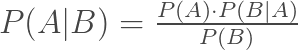
Deriving The Formula

We know what the Bayes formula is, but how can we derive it? To derive the Bayes Theorem formula, let’s start with a probability axiom that we know well:

So the probability of both A and B is the probability of B * probability of A, given B; or the probability of A * probability of B, given A.

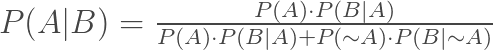
If we combine these equations, we get

If we divide both by P(B), we get

This is Bayes theorem.

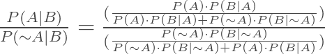
If we want the odds form, we first establish that

From this we deduce that P(A|B) =

And similarly P(~A|B) =

If we divide P(A|B) by P(~A|B), we get

By simplifying the a/b/c/b form to a/b * b/c, we get a/c, i.e.

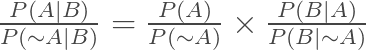
which is essentially Bayes Theorem in odds form. This form is used for computing a Bayesian updated.

Application of Bayes Theorem to Machine Learning

Naive Bayes is a supervised machine learning classification algorithm based on Bayes Theorem. This is an implementation of Naive Bayes from scratch in python, inspired by one of my favorite data scientists of all time, Chris Albon!

# Importing libraries
import pandas as pd
import numpy as np

# Create the data
data = pd.DataFrame()
data['job'] = ['writer','writer','writer','writer','engineer','engineer','engineer','engineer']
data['hours_worked'] = [84,52.5,91.2,45.4,94.2,89.9,90.2,40.8]
data['salary_in_k'] = [55,40,120,75,180,210,170,220]
data['office_on_floor'] = [2,1,9,4,2,10,8,15]

# Person to predict job for
person = pd.DataFrame()
person['hours_worked'] = [88]
person['salary_in_k'] = [180]
person['office_on_floor'] = [7]

Python

Using Bayes theorem, we see that

where:

job is the gender, writer or engineer
data is a collection of the features that comprise a person (hours_worked, salary_in_k, office on floor)
p(job) is the prior probability
p(job|data) is the posterior probability
p(data|job) is the likelihood

In Naive Bayes, we calculate the posterior probabilities for every class for every person, we then pick the largest probability and assign that class, i.e. job, to the datapoint, i.e. the person. So we calculate P(writer|data) and P(engineer|data) for each person.

Now let’s do that in code!

Calculate Prior Probabilities

n_writer = data['job'][data['job'] == 'writer'].count()
n_engineer = data['job'][data['job'] == 'engineer'].count()
total_ppl = data['job'].count()

# Probability of writer
P_writer = n_writer/total_ppl

# Probability of engineer
P_engineer = n_engineer/total_ppl

Calculate Likelihood

# Group by job, calculate mean and variance of each feature
data_means = data.groupby('job').mean()
data_variance = data.groupby('job').var()

# Mean - writer
writer_avg_hours_worked_mean = data_means['avg_hours_worked'][data_variance.index == 'writer'].values[0]
writer_salary_in_k_mean = data_means['salary_in_k'][data_variance.index == 'writer'].values[0]
writer_office_on_floor_mean = data_means['office_on_floor'][data_variance.index == 'writer'].values[0]

# Mean - engineer
engineer_avg_hours_worked_mean = data_means['avg_hours_worked'][data_variance.index == 'engineer'].values[0]
engineer_salary_in_k_mean = data_means['salary_in_k'][data_variance.index == 'engineer'].values[0]
engineer_office_on_floor_mean = data_means['office_on_floor'][data_variance.index == 'engineer'].values[0]

# Variance - writer
writer_avg_hours_worked_variance = data_variance['avg_hours_worked'][data_variance.index == 'writer'].values[0]
writer_salary_in_k_variance = data_variance['salary_in_k'][data_variance.index == 'writer'].values[0]
writer_office_on_floor_variance = data_variance['office_on_floor'][data_variance.index == 'writer'].values[0]

# Variance - engineer
engineer_avg_hours_worked_variance = data_variance['avg_hours_worked'][data_variance.index == 'engineer'].values[0]
engineer_salary_in_k_variance = data_variance['salary_in_k'][data_variance.index == 'engineer'].values[0]
engineer_office_on_floor_variance = data_variance['office_on_floor'][data_variance.index == 'engineer'].values[0]

# Calculate p(x | y):
def p_x_given_y(x, mean_y, variance_y):
    p = 1/(np.sqrt(2*np.pi*variance_y)) * np.exp((-(x-mean_y)**2)/(2*variance_y))
    return p

Excellent, we have our classifier! Now it’s time to use the classifier to make some predictions!

Get predictions using Naive Bayes Classifier

# Probability of P(writer|data)
P_writer * 
p_x_given_y(person['avg_hours_worked'][0], writer_avg_hours_worked_mean, writer_avg_hours_worked_variance) * 
p_x_given_y(person['salary_in_k'][0], writer_salary_in_k_mean, writer_salary_in_k_variance) * 
p_x_given_y(person['office_on_floor'][0], writer_office_on_floor_mean, writer_office_on_floor_variance)

**Outputs: 0.0027**

# Probability of P(engineer|data)
P_engineer * 
p_x_given_y(person['avg_hours_worked'][0], engineer_avg_hours_worked_mean, engineer_avg_hours_worked_variance) * 
p_x_given_y(person['salary_in_k'][0], engineer_salary_in_k_mean, engineer_salary_in_k_variance) * 
p_x_given_y(person['office_on_floor'][0], engineer_office_on_floor_mean, engineer_office_on_floor_variance)

**Outputs: 12.79**

Because P(engineer|data) > P(writer|data), we make the prediction that the person is an engineer!

Alternatively, we can simply use the Naive Bayes classifier that ships with sklearn

from sklearn.naive_bayes import MultinomialNB
naive_bayes = MultinomialNB()
# Train model
naive_bayes.fit(training_data, y_train)
# Get predictions
predictions = naive_bayes.predict(testing_data)

# Measure accuracy
from sklearn.metrics import accuracy_score, precision_score, recall_score, f1_score
print('Accuracy score: ', format(accuracy_score(y_test, predictions)))
print('Precision score: ', format(precision_score(y_test, predictions)))
print('Recall score: ', format(recall_score(y_test, predictions)))
print('F1 score: ', format(f1_score(y_test, predictions)))

Accuracy score:  0.9885139985642498
Precision score:  0.9720670391061452
Recall score:  0.9405405405405406
F1 score:  0.9560439560439562

And that is how Bayes Theorem is used in machine learning! In real life, we just feed it with more complex features, but the essence and the steps followed are the same as what we created above.

Now it’s your turn, I encourage you to take a problem from your life an apply Bayes Theorem to it!

Thank you for making it to the end of this post, as a reward, here’s a video of dogs meeting cute baby animals, you’ve earned it! 😇