

WHAT IS
MATH AND POLITICS TRIVIA
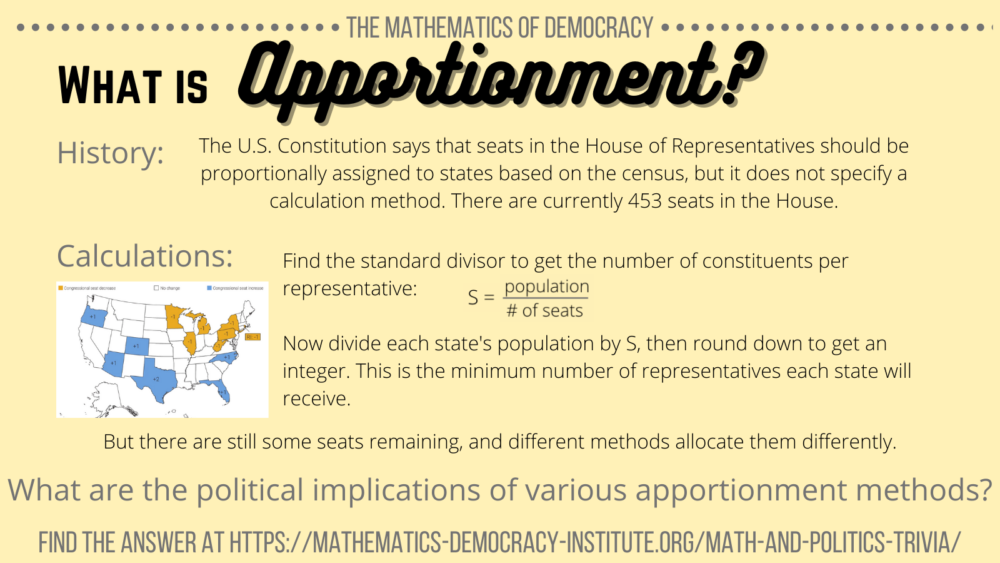
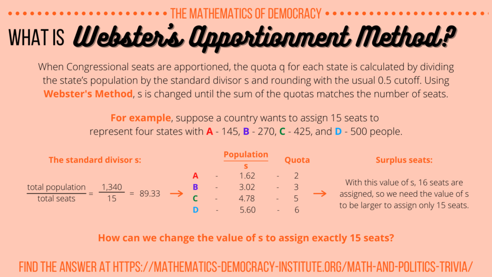
The importance of the apportionment of seats in the U.S. House of Representatives is often underestimated. Seats are only reallocated once every ten years based on the census, so apportionment decisions can have long-lasting consequences.
The total number of representatives was permanently set as 435 in 1929 (given an ever-changing population, this number is largely arbitrary today). Each state receives a minimum number of those 435 representatives; this minimum is obtained by rounding down the quotient of the state’s population by the standard divisor (ideal amount of people per representative). This does not account for all 435 representatives, and the remaining seats have to be allocated according to some method.
Throughout U.S. history, various procedures, proposed by Hamilton, Jefferson, and Webster among others, have been used for allocation of remaining seats. The dispute over the initial method even caused the first ever presidential veto by George Washington! A method based on the geometric mean, due to Huntington and Hill, is currently in use. There is no agreement among mathematicians that Huntington-Hill is the best possible way to apportion House seats.
Different methods of apportionment allocate seats differently, and this means that some states might be overrepresented or underrepresented in Congress. This disparity carries over to the Electoral College, since the number of each state’s electoral votes is based on the size of its congressional delegation. For more on the Electoral College, see our previous trivia.
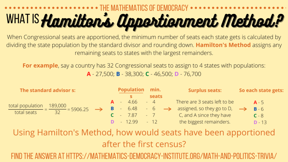
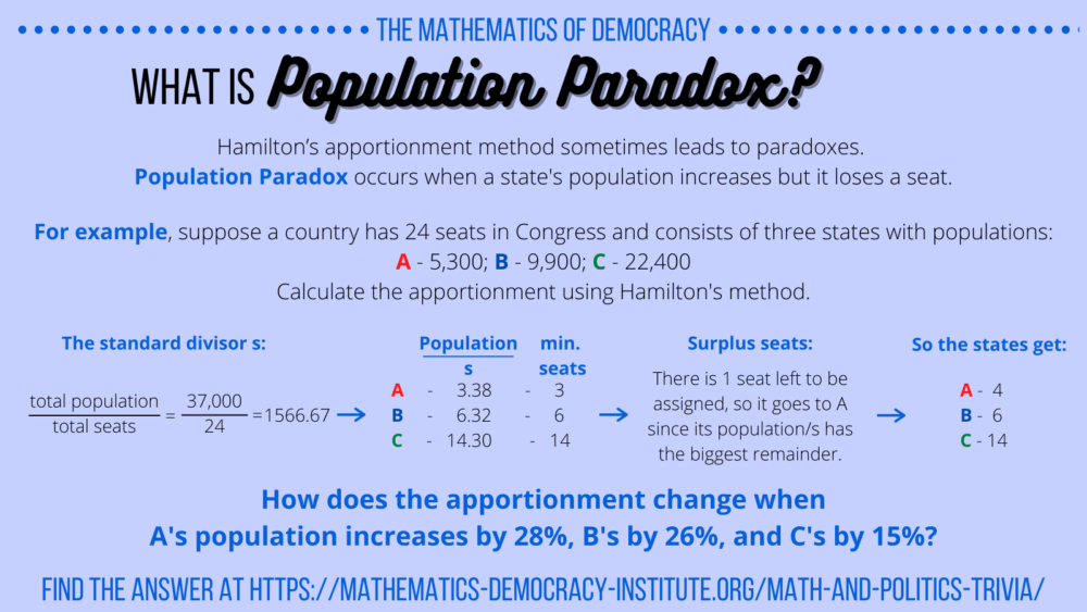
After the first census was conducted in 1790, the US government needed a method to apportion congressional seats, so Alexander Hamilton proposed his method in 1791. Congress approved a bill for the House of Representative to have 120 representatives and for the use of Hamilton’s method. According to the census, the total population at the time was 3,893,635, so the standard divisor is calculated as:
s = total population/total seats = 3,893,635/120 = 32,446.958
Therefore, using Hamilton’s Method, the seats would have been assigned this way:
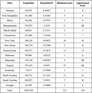
While Hamilton’s Method was adopted by Congress, Washington vetoed the decision, the first presidential veto ever used. Washington may have done this because Jefferson’s alternative method gave his home state of Virginia an extra representative. Later, Hamilton’s Method was readopted and used from 1852 until 1911.
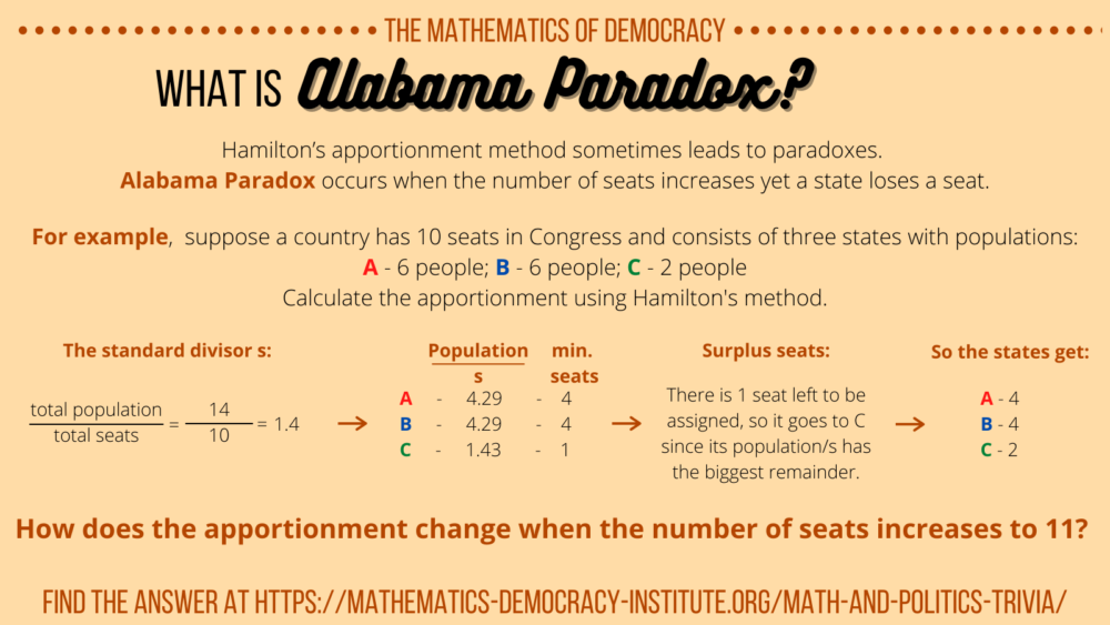
One of Hamilton Method’s advantages is that it does not violate the quota rule, a desirable property of apportionment where the number of seats a state receives is the rounding, up or down, of its total population divided by the standard divisor. This means that each representative represents approximately the same number of people. Additionally, Hamilton’s method is straightforward and easy to understand. However, this simplicity is also its downfall because Hamilton’s method can produce strange and counterintuitive apportionments. These are known as the Alabama paradox, new states paradox, and the population paradox. Stay tuned for future trivia posts on these topics!
To find the power index for each voter, we must look at every possible sequential coalition (order matters!). Here, the sum is in blue until the quota of 16 is cleared. The last blue voter is pivotal.
To start, we recalculate the standard divisor s = total population/total number of seats = 14/11 = 1.27. Therefore we get:
There are two seats that remain to be allocated, so they go to A and B since they have the biggest remainders. This means the final allocation of seats is:
Even though the number of seats increased, state C lost a seat!
The Alabama Paradox was first observed after the 1882 census. During the mid-19th century, the United States experienced a population boom with 14 states joining the country. The number of seats in the House of Representatives increased from 234 to 386 between 1856 and 1902. To compensate for these changing populations, in 1882 the US Census calculated all possible apportionments of Congressional seats using Hamilton’s method for every house size between 275 and 350 seats. They first noticed this paradox when Alabama lost a seat in the calculations between the House sizes of 299 and 300:
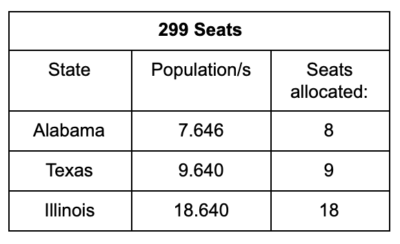
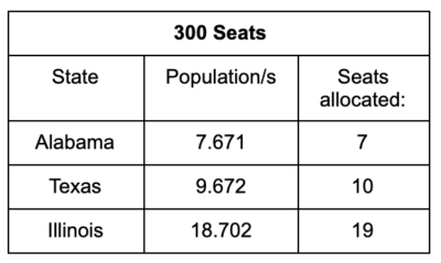
Why did the Alabama Paradox occur? When the seats were increased to 300, each state population was divided by a smaller standard divisor s than when there were 299 seats. When the denominator gets smaller, the fraction gets bigger, so each state’s population/s increases by about 0.33%. However, since Illinois and Texas started with larger populations, this change is more significant for them than Alabama. This caused the two larger states to see an increase that was larger than that of Alabama, with their decimal part overtaking Alabama’s.
Ultimately, Congress decided to continue using Hamilton’s Method with a House of 325 members, a size at which this paradox did not occur. However, this problem reappeared in 1902. Again, the Census Bureau recalculated the apportionments for all possible House sizes between 350 and 400 seats, revealing a host of issues related to the Alabama Paradox: Maine got 3 seats for house sizes of 350–382, 386, 389–390, but 4 seats at all other sizes, and Colorado got 3 seats except when it lost a seat with with a House of 357 members. Representative John Littlefield of Maine went so far as to say, “God help the State of Maine when mathematics reach for her and undertake to strike her down.” The debate became so substantial that Hamilton’s method was ultimately abandoned in favor of Webster’s method, a topic we’ll cover in a future trivia post.
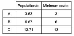
After the population increase, the populations are now: A: 6,800, B: 12,500, and C: 27,500. Now recalculate the apportionment. The new standard divisor equals
total population/total seats = 45,000/24 = 1875
To start, we recalculate the standard divisor s = total population/total number of seats = 14/11 = 1.27. Therefore we get:
There are two seats that remain to be allocated, so they go to B and C since they have the biggest remainders. This means the final allocation of seats is:
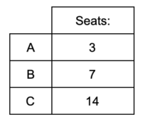
Notice that even though A had the largest population growth, it lost a seat!
The population paradox was first observed in the early 20th century: In 1900, seats were reapportioned following the latest census. Virginia’s population/s was large enough that Virginia got an extra seat whereas Maine did not.
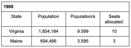
Over the following year, the United States experienced substantial population growth: Virginia’s population grew by 19,767 and Maine’s by 4,648. If House representatives had been reapportioned that year, we would have
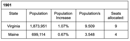
Even though Virginia’s population grew more than Maine’s, Virginia still would have lost a seat to Maine.
This paradox is rooted in two issues: first, the number of seats in Congress has not necessarily kept up with population growth (in fact, it has been fixed at 435 since 1940). Thus, anytime one state’s population grows to warrant an extra representative, it must take a seat away from another state. Also, decimal remainders do not reflect relative size when comparing two different state populations/s. Due to paradoxes like this, Hamilton’s method was eventually abandoned in favor of more mathematically “fair” apportionment methods. Stay tuned to learn more about these methods in future trivia posts.
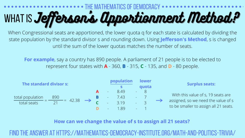
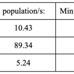
We want to assign all 21 seats, so the divisor s should be smaller, making each value of population/s larger. Let’s try something convenient, say s=42.
That didn’t help allocate any of the remaining seats, so we need s to be even smaller. Let’s try s=40. This means we have:
This works, and all 21 seats have been assigned!
This method of apportionment was proposed by Thomas Jefferson in 1791 as an alternative to Hamilton’s method. It was used to allocate Congressional seats in the United States from 1792-1842, after George Washington vetoed Hamilton’s proposal. Though Jefferson’s method avoids some of the paradoxes we see in Hamilton’s method, it has some pitfalls of its own. First, finding the correct value to use for s is often done by trial and error, a potentially inefficient process. Also, this apportionment method tends to favor larger states. Some speculate that Washington initially chose this method over Hamilton’s because it gave his home state of Virginia, a large state at the time, an extra seat.
Jefferson’s method also fails the quota rule, the idea that the number of seats a state gets should be its population/s rounded either up or down. For example, let’s say we have a population of 1,229,000 and there are 57 seats to apportion. This means s=1,229,000/57=21,651.4.
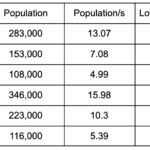
This value of s only assigns 54 of the 57 seats, so let’s try s=20,300.
Now we have assigned all 57 seats, but notice that state D ends up with 17 seats. Since D’s population divided by the original value of s was 15.98, the quota rule states that D should be assigned either 15 or 16 seats. This illustrates the failure of Jefferson’s method to satisfy the quota rule.
First, we need to recalculate s to include the new population and seats: s=105,250/105=1,002.38.
Since there is one more seat to assign, it goes to state A since it has the largest remainder. Therefore, each state gets:
A – 11
B – 89
C – 5 seats.
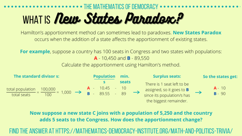
The new state C got exactly 5 seats, the amount that was added to the Congress. However, the apportionment of the other 100 seats changed just from the addition of the new state. This is a prime example of the new states paradox, a phenomenon that was first observed in 1907 when Oklahoma became the 46th state. At the time, the existing 45 states had a combined population of about 75 million and 386 seats in Congress, and Oklahoma’s 1 million citizens corresponded to about 5 representatives. To avoid complications like the Alabama paradox and the population paradox, 5 seats were added to Congress when Oklahoma joined the union. As expected, when the apportionment was calculated, Oklahoma got those extra five seats. However, New York lost a seat to Maine, even though neither of their populations changed:
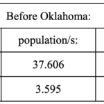
Since the remainder of New York’s population/s was bigger than Maine’s, New York was allocated an extra seat.
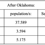
After Oklahoma and the extra seats were included in the calculation, the fractional parts of the population/s for each state decreased. Since New York’s population/s was greater than Maine’s, its fraction decreased more, enough to give Maine the extra seat.
While the Alabama paradox was avoided by permanently setting the number of representatives, and the population paradox was only found through experimenting with calculations, the new states paradox was a problem that could not be controlled by Congress. In 1911, soon after the discovery of the new states paradox, Hamilton’s method was abandoned.
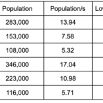
We need s to be larger, so let’s try s=11,000. Now we get:
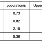
The number of assigned seats remained unchanged, so we need s to be even higher. Let’s try s=12,000.
Now we’ve assigned too few seats. Since we want just the apportionment of either C or D to change, let’s lower s slightly and try =11,800.
Finally, this value of s assigns exactly 10 seats. Therefore, using Adams’ apportionment method, the states get: A – 1; B – 1; C – 3; D – 5 seats. Let’s compare this to Jefferson’s method. The two calculations differ, because Adams’ method always rounds up while Jefferson’s method rounds down. In this example, using s=8,250, we get:
Observe that, under Jefferson’s method, the state with the largest population, D, got more seats, while A, the state with the smallest population, lost a seat. This is true in general – Adams’ method favors smaller states and larger states have the advantage under Jefferson’s method. Since Adams’ method prioritizes small states, it can sometimes violate the quota rule: a state can be assigned a number of seats that is not their population divided by the original s rounded up or down. However, unlike with Jefferson’s method, every state will always be assigned at least one representative, a Constitutional requirement.
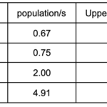
Since the original s value assigned 16 seats, we need s to be slightly larger to only assign 15. Let’s try s=90.
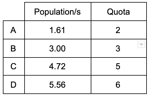
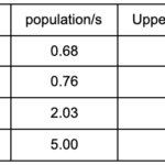
This s value still assigned a total of 16 seats, so we need s to be even larger. This time, let’s use s=92.
Finally, this value of s assigns the correct amount of seats!
Webster’s method, like Jefferson’s method, is a divisor method since it changes the value of s until the desired number of seats are apportioned. They therefore share some of the same properties. For example, both methods may fail the quota rule and tend to favor larger states. But the methods differ on how they round each state’s quota: Jefferson’s method rounds the quotas down, while Webster’s method uses the usual 0.5 rounding cutoff. Due to this difference, Webster’s method faces these complications much less often: with Webster’s method, it is much more likely a state will receive its original quota rounded either up or down, and big states are at less of an advantage. In fact, when Congress began to have concerns over the preferential treatment of big states under Jefferson’s method, they adopted Webster’s method instead in 1842. In 1852, it was replaced by Hamilton’s method, but Webster’s was adopted yet again and used from 1910-1940 after the paradoxes of Hamilton’s method became apparent.
Webster’s method uses the arithmetic mean (half way between two successive integers) as the cutoff for rounding, but there are other ways to decide where to cut off. Stay tuned for future trivia posts, where we’ll explore other apportionment methods, including the one still used today.
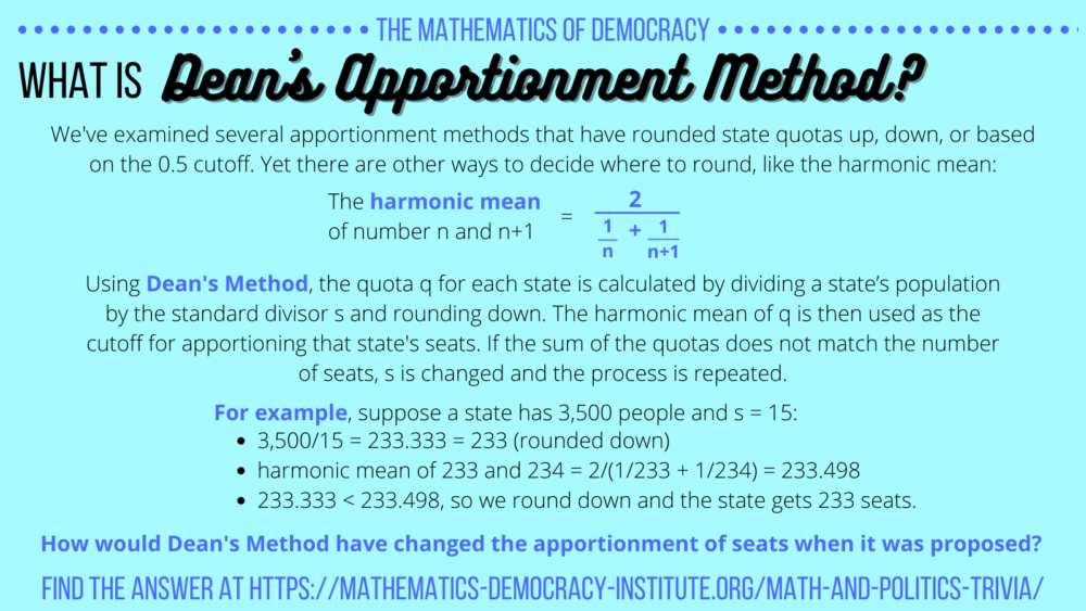
James Dean proposed his apportionment method in 1832. At the time, the United States had 24 states with a total population of 11,931,000 and 240 House of Representative seats. Here’s how he proposed those seats be apportioned:
s=11,931,000/240=49,712.5.
| State: | Population: | Population/s: | Round down: | Harmonic mean: | Apportionment: |
| NY | 1,918,578 | 38.59347247 | 38 | 38.49350649 | 39 |
| PA | 1,348,072 | 27.11736485 | 27 | 27.49090909 | 27 |
| VA | 1,023,503 | 20.58844355 | 20 | 20.48780488 | 21 |
| OH | 937,901 | 18.86650239 | 18 | 18.48648649 | 19 |
| NC | 639,747 | 12.86893638 | 12 | 12.48 | 13 |
| TN | 625,263 | 12.57758109 | 12 | 12.48 | 13 |
| KY | 621,832 | 12.50856424 | 12 | 12.48 | 13 |
| MA | 610,408 | 12.27876289 | 12 | 12.48 | 12 |
| SC | 455,025 | 9.1531305 | 9 | 9.473684211 | 9 |
| GA | 429,811 | 8.645934121 | 8 | 8.470588235 | 9 |
| MD | 405,843 | 8.163801861 | 8 | 8.470588235 | 8 |
| ME | 399,454 | 8.035282877 | 8 | 8.470588235 | 8 |
| IN | 343,031 | 6.900296706 | 6 | 6.461538462 | 7 |
| NJ | 319,922 | 6.435443802 | 6 | 6.461538462 | 6 |
| CT | 297,665 | 5.987729444 | 5 | 5.454545455 | 6 |
| VT | 280,657 | 5.645602213 | 5 | 5.454545455 | 6 |
| NH | 269,326 | 5.417671612 | 5 | 5.454545455 | 5 |
| AL | 262,508 | 5.280523007 | 5 | 5.454545455 | 5 |
| LA | 171,904 | 3.457963289 | 3 | 3.428571429 | 4 |
| IL | 157,147 | 3.161116419 | 3 | 3.428571429 | 3 |
| MO | 130,419 | 2.623464923 | 2 | 2.4 | 3 |
| MS | 110,358 | 2.219924566 | 2 | 2.4 | 2 |
| RI | 97,194 | 1.955121951 | 1 | 1.333333333 | 2 |
| DE | 75,432 | 1.517364848 | 1 | 1.333333333 | 2 |
| Total: | 242 |
Since slightly too many seats are apportioned, we have to use a larger s. Let’s try s = 49,900.
| State: | Population: | Population/s: | Round down: | Harmonic mean: | Apportionment: |
| NY | 1,918,578 | 38.44845691 | 38 | 38.49350649 | 38 |
| PA | 1,348,072 | 27.01547094 | 27 | 27.49090909 | 27 |
| VA | 1,023,503 | 20.51108216 | 20 | 20.48780488 | 21 |
| OH | 937,901 | 18.79561122 | 18 | 18.48648649 | 19 |
| NC | 639,747 | 12.82058116 | 12 | 12.48 | 13 |
| TN | 625,263 | 12.53032064 | 12 | 12.48 | 13 |
| KY | 621,832 | 12.46156313 | 12 | 12.48 | 12 |
| MA | 610,408 | 12.23262525 | 12 | 12.48 | 12 |
| SC | 455,025 | 9.118737475 | 9 | 9.473684211 | 9 |
| GA | 429,811 | 8.613446894 | 8 | 8.470588235 | 9 |
| MD | 405,843 | 8.133126253 | 8 | 8.470588235 | 8 |
| ME | 399,454 | 8.00509018 | 8 | 8.470588235 | 8 |
| IN | 343,031 | 6.874368737 | 6 | 6.461538462 | 7 |
| NJ | 319,922 | 6.411262525 | 6 | 6.461538462 | 6 |
| CT | 297,665 | 5.965230461 | 5 | 5.454545455 | 6 |
| VT | 280,657 | 5.624388778 | 5 | 5.454545455 | 6 |
| NH | 269,326 | 5.397314629 | 5 | 5.454545455 | 5 |
| AL | 262,508 | 5.260681363 | 5 | 5.454545455 | 5 |
| LA | 171,904 | 3.44496994 | 3 | 3.428571429 | 4 |
| IL | 157,147 | 3.149238477 | 3 | 3.428571429 | 3 |
| MO | 130,419 | 2.613607214 | 2 | 2.4 | 3 |
| MS | 110,358 | 2.211583166 | 2 | 2.4 | 2 |
| RI | 97,194 | 1.947775551 | 1 | 1.333333333 | 2 |
| DE | 75,432 | 1.511663327 | 1 | 1.333333333 | 2 |
| Total: | 240 |
As opposed to the actual apportionment method used in 1832, under Dean’s method, states such as New York, Pennsylvania, and Virginia would have lost seats, whereas states like Delaware, Missouri, and Louisiana would have gained some. In practice, Dean’s method has never actually been used to apportion seats in the United States House of Representatives. However, when facing the loss of a seat after the 1990 census, Montana politicians did argue for its adoption.
Dean’s method is quite similar to other apportionment methods we’ve seen, such as Jefferson’s, Adam’s, and Webster’s. The only difference is in the use of the harmonic mean. Observe the differences between the rounding cutoffs used in each method:
| Rounding Down
(Jefferson’s) |
Rounding up
(Adam’s) |
0.5 Cutoff
(Webster’s) |
Harmonic Rounding
(Dean’s) |
|
| 0-1 | 1 | 0 | 0.5 | 0 |
| 1-2 | 2 | 1 | 1.5 | 1.333 |
| 2-3 | 3 | 2 | 2.5 | 2.400 |
| 3-4 | 4 | 3 | 3.5 | 3.429 |
| 4-5 | 5 | 4 | 4.5 | 4.444 |
| 5-6 | 6 | 5 | 5.5 | 5.455 |
| 6-7 | 7 | 6 | 6.5 | 6.462 |
| 7-8 | 8 | 7 | 7.5 | 7.467 |
In the table above, we see that the smaller numbers tend to have harmonic means with a smaller decimal. This means there is a lower cutoff for states with smaller populations to gain an extra seat, an advantage for small states.
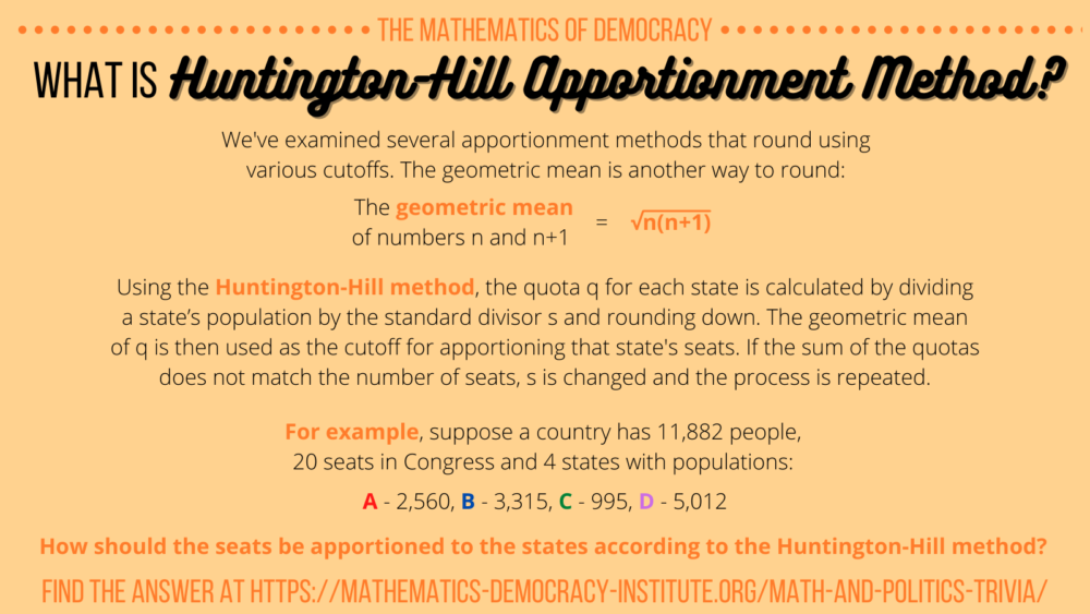
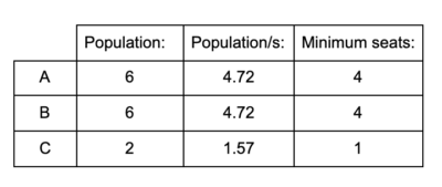
We start by calculating s = total population/total number of seats = 11, 882/20 = 594.1. Then we can look at how this affects each state:
| State | population/s | population/s, rounded down |
| A | 4.31 | 4 |
| B | 5.58 | 5 |
| C | 1.67 | 1 |
| D | 8.44 | 8 |
Now we can calculate the geometric means for each of the rounded down numbers:
| Number | Geometric mean |
| 4 | √(4 · 5) = 4.47 |
| 5 | √(5 · 6) = 5.48 |
| 1 | √(1 · 2) = 1.41 |
| 8 | √(8 · 9) = 8.49 |
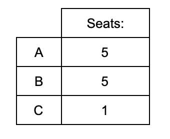
Finally, we compare the population/s to the geometric means. Anytime the population/s is greater than the geometric mean, we round it up. If it’s less than the mean, we round down:
| State | population/s vs geometric mean | Seats allocated |
| A | 4.31 < 4.47 | 4 |
| B | 5.58 > 5.48 | 6 |
| C | 1.67 > 1.41 | 2 |
| D | 8.44 < 8.49 | 8 |
All 20 seats have been allocated! This is an advantage of the Huntington-Hill method: it often allocates exactly the number of available seats, so s does not need to be changed.
This apportionment method is similar to both the Webster and Dean methods, though they all round in different ways. Like the other methods, Huntington-Hill tends to give smaller states an advantage. The geometric mean produces numbers smaller than the usual 0.5 cutoff and this difference is more pronounced in smaller numbers, so it is easier for small states to clear the rounding cutoff. This means that the Huntington-Hill method has a stronger bias for smaller states than the Webster method. However, since the geometric mean is closer to the 0.5 cutoff than the harmonic mean used in the Dean method, there is less bias in the Huntington-Hill method than in the Dean method.
Huntington-Hill method was first proposed by members of the Census Bureau in the 1920’s. Though it gained traction, it was never used during that decade, because it would have changed the apportionment of six states, negatively impacting primarily large states. Through the 1930’s, both Webster and Huntington-Hill methods were used to apportion American Congressional seats. However, in 1941, the calculations differed, with Webster assigning 6 seats to Arkansas and 18 to Michigan, versus Huntington-Hill’s 7 to Arkansas and 17 to Michigan. A representative from Arkansas successfully campaigned to make Huntington-Hill the permanent apportionment method. Huntington-Hill was then adopted in the 1941 Apportionment Act and is still used today. (That act also permanently set the number of House seats at 435.)
It’s important to note how each of the methods we’ve explored so far fails the Balinski-Young Theorem. First, as we saw, Hamilton’s method is susceptible to a host of paradoxes, including the population paradox. However, one advantage is that it always satisfies the quota rule. In contrast, the Jefferson, Adams, Webster, Dean, and Huntington-Hill methods are all “divisor methods” because they change the standard divisor s to apportion seats. All divisor methods can violate the quota rule, but they always avoid paradoxes. Additionally, all of the methods we’ve seen so far are neutral.
In the mid 1980’s, mathematicians Michel Balinski and Peyton Young searched for an apportionment system that had the best of both worlds, satisfying the quota rule and avoiding paradoxes. They constructed a system that satisfies the quota rule and is free of the Alabama paradox, but it can have the population paradox. This method has many desirable properties, but it is not used very often. Using a structure similar to the proof of Arrow’s Impossibility Theorem, they proved that an apportionment method satisfying all of these desirable properties can never exist.
After their proof, Balinski and Young argued that the best of the existing apportionment methods is Webster’s. Most experts agree with this: even though Webster is a divisor method that is capable of failing the quota rule, it is less susceptible to failure than other existing divisor methods. In fact, had Congressional seats been apportioned with Webster’s method for all of American history, the quota rule would have always been satisfied. Despite this evidence, the Huntington-Hill method is still used for American apportionment.
