Stage
Modality
Delivery technique
Dose calculation
Early
Ortovolt – X ray
Conventional
Experiment based
Intermediate
Co – 60, low-energy Linac
2D and 3D conformal
Pencil beam
Advanced
High-energy Linac
IMRT
Pencil beam convolution
Superposition
Monte Carlo
Analytical anisotropical algorithm (AAA)
Boltzmann-based method
Regarding the delivery techniques in radiotherapy, Fig. 8.1 shows illustrations on how the delivery techniques evolved. In the early stage, the external beams were implemented with a limited number of fields and arranged in simple ways that could be regularly repeated from case to case. The evolution on computer technologies brings also the influence into the delivery techniques in radiotherapy. In 1988, Andre Brahme had proposed a theory to modulate the fluence of beam radiation through the inverse method (Brahme 1988). This technique became a well-known technique which was called IMRT technique. However, the clinical implementation of this technique can be done around 12 years after Brahme’s work (Webb 2005).
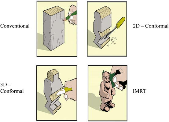
Fig. 8.1
The dose sculpting to illustrate the evolution of delivery techniques (Modified from John Schreiner 2006)
Nowadays, IMRT has many derivations. Regarding the radiation source, IMRT can be implemented not only for photons but also for other particles such as proton and electron. IMRT also evolves its technique with various methods. One of the new techniques has used image confirmation of the targets during treatment, namely, image-guided radiation therapy (IGRT) (Jaffray 2005). The other new technique based on the high-precision accelerated stereotactic modality is called stereotactic radiation therapy/surgery (SRT/S) (Blomgren et al. 1995; Hamilton et al. 1995). The newest delivery technique in IMRT was named intensity-modulated arc therapy (IMAT). These techniques implement rotational cone beams of varying shapes to achieve intensity modulations (Yu 1995). In this chapter, the discussion is focused only on the basic IMRT technique.
8.1 3D Conformal Radiation Therapy Versus IMRT
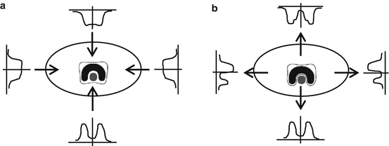
To understand the advantage of IMRT technique, it can be started by comparison between the 3D conformal radiation therapy (3DCRT) and IMRT (Webb 2000; Schlegel and Mahr 2001; Sternick 1997). Figure 8.2b shows that the IMRT is based on the inverse method to achieve the best dose distribution on the target. It differs from the 3DCRT which is based on forward method (Fig. 8.2a). IMRT has reformed the aims of treatment planning from the design of fields to the design of dose distributions.
IMRT also changes the paradigms in radiotherapy. Based on ICRU-50 recommendation, the dose distribution on the planning target volume (PTV) that is produced by 3DCRT should be uniformed (ICRU 50, 1993). But IMRT does not need to produce the uniform dose distribution on PTV. In the IMRT method, the ability to vary the fluence of radiation across the surface of the beam plays an important role. The IMRT technique should not produce the beams whose intensity is either uniform or changes uniformly, such as by the addition of a wedge filter. The other paradigm is also shifted in IMRT, namely, the dose at isocenter. In 3DCRT, the dose at isocenter should be reported but not in IMRT. The dose at isocenter in IMRT became an insignificant parameter. Table 8.2 shows the detailed comparison between the paradigms in 3DCRT and IMRT.
Table 8.2
The paradigms in 3DCRT and IMRT
3DCRT | IMRT | |
|---|---|---|
Dose calculation | Forward method | Inverse method |
Field composition | Simple | Complex |
Region of interest (ROI) | No need to define | Target and organs at risk |
Fluence distribution | Uniform | Nonuniform |
Dose distribution | Uniform | High gradient |
Monitor unit | Low | High |
8.2 IMRT Terminology
As on the previous discussion, the IMRT method provides better dose distribution than 3DCRT method. Unfortunately, even with IMRT, it is impossible to deliver 100 % dose in target and 0 % in organs at risk. Bortfeld et al. confirmed that it is infeasible to make true inverse dose planning in IMRT. In this section, the IMRT terminology will be discussed. It is related to the physical variables that will be optimized and should be defined.
The first variable that should be optimized is the number of beams and their beam angles. Figure 8.3 shows the illustration of the number of beams and beam angles. The number of beams and beam angles depends on many factors such as anatomy, radiation tolerance, and the prescribed dose of target. Based on the image reconstruction in the CT scan, the early theoretical approaches to inverse planning assumed a very high number of coplanar beams (Brahme et al. 1982). It is related that the higher the number of beams is, the higher the dose conformation potential is. But Söderström and Brahme 1995 suggested using no more than three beams. Therefore, the question about the “optimum” number of beams in IMRT has been discussed frequently in the literature among the researchers (Brahme 1993, 1994; Mackie et al. 1994; Mohan and Ling 1995; Mohan and Wang 1996; Söderström and Brahme 1996). Regarding the optimization of orientation and the number of beams, it should be noted that the noncoplanar beams are unusually used in IMRT and the parallel-opposed beam should also be avoided (Stein et al. 1997).
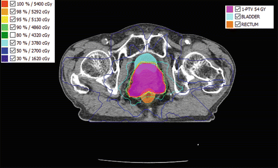
Fig. 8.3
An IMRT dose distribution for a prostate cancer from seven beam angles, namely, 25°, 85°, 129°, 180°, 223°, 275°, and 335°
In IMRT, the second variable that should be optimized is the intensity map for each beam. Usually, each beam is divided into a number of small areas which are called beam elements (bixels or beamlets). Each bixel or beamlet has a typical size of 0.5 × 0.5 to 1 × 1 cm2, and the number of bixels or beamlets for all beams is normally in the order of 1000–10,000. Because it could be very difficult to deliver intensity-modulated beams directly with a linear accelerator (LINAC), the intensity maps are developed using a set configuration of multileaf collimator (MLC). One configuration of MLC is well known as segment. Figure 8.4 shows the illustration to understand bixels or beamlets and segments. Therefore, finding the best intensity maps is not only a high-dimensional problem in optimization but also a complex problem in “leaf sequencing.” Many methods and techniques to optimize intensity maps have been developed and implemented (Cho and Marks 2000; Alber and Nüsslin 2001).
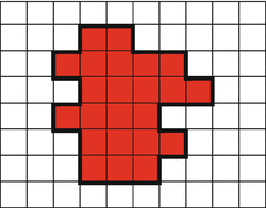
Fig. 8.4
One segment (red areas) consists of 23 bixels or beamlets
Instead of the intermediate step of using intensity maps altogether, there are two research groups that suggested to directly optimize MLC shapes (apertures) and their weights (DeNeve et al. 1996; Shepard et al. 2002). Based on the anatomy of the target or organs at risk, the MLC shapes can be generated. But the MLC shapes can be directly optimized together with the weights of the segments. The direct optimization of MLC shapes and weights becomes mathematically a difficult, non-convex problem.
The last optimization is related to the number of intensity levels. Many researchers agree that IMRT planning methods assume a continuous modulation of the intensity. But there are several researchers who have another idea to use a different approach. They suggested that promising results can be achieved “discreetly” like beam profile as well (Bortfeld et al. 1994a; Gustafsson et al. 1994; DeNeve et al. 1996). In fact, the results show no significant difference between using a moderate number of stairstep with 5–20 “intensity levels” in each beam profile and continuous modulation (Keller-Reichenbecher et al. Keller-Reichenbecher et al. 1999). Figure 8.5 shows the intensity levels that are produced by both methods. Therefore, it is unnecessary to use fully dynamic method in IMRT with MLC. To avoid the high-dose delivery to patients, IMRT can be realized in a step-and-shoot method. This method delivers the beams based on a number of static MLC-shaped segments from each direction of incidence. By this way, the total number of beam segments that is delivered is in the order of 100. Nowadays, the linac machine can implement this method automatically and quickly. More detailed information about the comparison of the features of dynamic versus step-and-shoot IMRT can be found in the publication from Chui et al. (2001).
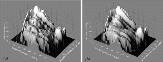
Fig. 8.5
The intensity levels based on the step-and-shoot method (a) and the sliding windows method (b)
8.3 Inverse Planning Techniques
After the discussion about the variables to be optimized, the inverse planning techniques became the next topic to discuss. The advantages of IMRT can only be taken into account through the implementation of these techniques. Using inverse planning, the aims of the treatments are not only the desired dose distribution but also the desired biological end points. The plan parameters which best reflect the treatment’s aims are determined by optimization algorithms.
There are two well-known inverse planning techniques which are implemented in IMRT, namely, beamlet-based inverse planning and aperture-based inverse planning. The difference of both techniques is based on the treatment’s variables that are optimized. Beamlet-based inverse planning begins with dividing the field into a grid of beamlets, and then the weights of these beamlets are optimized. The intensity map, which is a distribution of the beamlet’s weights, is provided by the optimization. After the intensity maps are done, each intensity map is sequenced into a set of deliverable aperture shapes. Figure 8.6 shows the illustration of the two steps on the beamlet-based inverse planning. On the other hand, aperture-based inverse planning does not have the sequencing step, while a set of deliverable apertures is already included in the optimization.
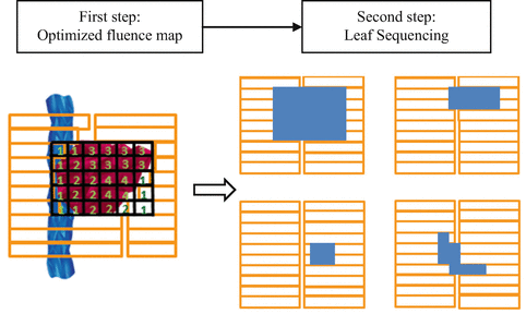
Fig. 8.6
An illustration of a two-step method on the beamlet-based inverse planning (Modified from Yu et al. 2006)
Many researchers proposed beamlet-based inverse planning based on two major step approaches to produce an optimized treatment plan. In the first step, the pencil beam intensities of each beamlets are optimized (Bortfeld et al. 1994b; Chui et al. 1994; Galvin et al. 1993; Webb 1994, 1998a, b). During this process, the quality of the treatment plan is recorded based on an objective function. In the second step, this technique applied the leaf sequencing algorithm to implement each optimized intensity map into a set of deliverable beam apertures (Xia and Verhey 1998; Crooks et al. 2002; Langer et al. 2001; Saw et al. 2001; Convery and Webb 1998).
However, some problem appears from this two-step process (intensity optimization and leaf sequencing) employed in the beamlet-based inverse planning process for MLC-based IMRT. Cho et al. reported that a large number of complex field shapes lead to a loss in efficiency and an increase in collimator artifacts (Cho and Marks 2000). Some researcher tries to simplify the delivery and smoothing the intensity maps, but a loss in treatment plan quality occurred (Alber and Nüsslin 2000; Spirou et al. 2001). The other researcher used a large number of segments with a low number of monitor units (MUs) along with small off-axis fields (van Santvoort and Heijmen 1996; Webb et al. 1997). This approach not only brings new challenges for accurate dose calculation and unrealistic requirements for geometry accuracy of the MLC and dosimetric accuracy of the linear accelerator (Budgell et al. 2000; LoSasso et al. 1998) but also needs an intensively quality assurance to achieve the well-established safety and accuracy standards (LoSasso et al. 1998).
Aperture-based inverse planning is made as an inverse planning technique to solve the complexity of IMRT treatment plans. Each aperture that is considered by optimization process is determined to satisfy the delivery constraints. There is no leaf sequencing and no need to divide the final intensity maps into discrete intensity level. For this planning, there are two methods that already developed, namely, contour-based treatment planning and direct aperture optimization.
There are two approaches in contour-based treatment planning to define the aperture shapes. The first approach is based on the patient’s anatomy (Xiao et al. 2000, 2003; Bednarz et al. 2002; Chen et al. 2002). Before the optimization, this approach constructed the aperture shapes based on a target and organ at risk for each beam angle from the beam’s eye view (BEV). After the first aperture shape is confirmed for the target and its appropriate margin, the additional apertures are added to protect any OAR regarding the first aperture shape. Figure 8.7 demonstrates an illustration of these processes. After the dose calculation, the aperture weights are optimized. There are several algorithms, which have been performed for optimization, such as a simultaneous projection algorithm (Xiao et al. 2000), a mixed integer algorithm (Bednarz et al. 2002), and an iterative least-square algorithm (Chen et al. 2002). To produce the additional apertures, DeGersem developed an anatomy-based segmentation tool (ABST) (DeGersem et al. 2001a, b). In the second approach, isodose curves can be used to perform a contour-based treatment planning. At William Beaumont Hospital, this approach has been developed to increase the dose uniformity with tangential breast radiotherapy (Kestin et al. 2000; Remouchamps et al. 2003).
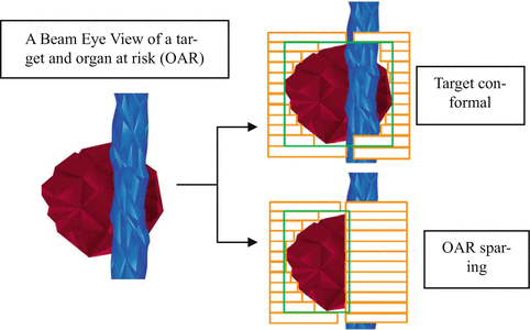
Fig. 8.7
 Computer-Aided Detection and Differentiation of Breast Cancer on Mammograms
 Computerized Prediction of Treatment Outcomes and Radiomics Analysis
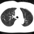 Computer-Aided Detection of Lung Cancer
 Computer-Assisted Treatment Planning Approaches for Carbon-Ion Beam Therapy
 Surface-Imaging-Based Patient Positioning in Radiation Therapy
 Computer-Assisted Target Volume Determination


An illustration of the processes to construct the aperture shapes based on a target and organ at risk from a beam’s eye of view (BEV) (Modified from St-Hilaire et al. 2009)
Related posts:
Computer-Aided Detection and Differentiation of Breast Cancer on Mammograms
Computerized Prediction of Treatment Outcomes and Radiomics Analysis
Computer-Aided Detection of Lung Cancer
Computer-Assisted Treatment Planning Approaches for Carbon-Ion Beam Therapy
Stay updated, free articles. Join our Telegram channel
Full access? Get Clinical Tree
