The Euler angle parameterization

The most popular representation of a rotation tensor is based on the use of three Euler angles. Early adopters include Lagrange, who used the newly defined angles in the late 1700s to parameterize the rotations of spinning tops and the Moon [1, 2], and Bryan, who used a set of Euler angles to parameterize the yaw, pitch, and roll of an airplane in the early 1900s [3]. Today, Euler angles are widely used in vehicle dynamics and orthopaedic biomechanics. As discussed in [4, 5], the Euler angle representation dates to works by Euler [6, 7] that he first presented in 1751. Although the paper [7] dates to the 18th century, it was first published posthumously in 1862. In Euler’s papers, he shows how three angles can be used to parameterize a rotation, and he also establishes expressions for the corotational components of the angular velocity vector.

Contents

The Euler angle sequence and Euler basis

One interpretation of the Euler angles involves a decomposition of a rotation tensor $\mathbf{R}$ into a product of three fairly simple rotations:

(1) $\begin{equation*} {\bf R} = \grave{\bf R}(\gamma^1, \, \gamma^2, \, \gamma^3) = {\bf L}\left(\gamma^3, \, {\bf g}_3\right){\bf L}\left(\gamma^2, \, {\bf g}_2\right){\bf L}\left(\gamma^1, \, {\bf g}_1\right), \end{equation*}$

where, from Euler’s representation,

(2) $\begin{equation*} {\bf L}(\theta, \, {\bf b}) = \cos(\theta)({\bf I} - {\bf b}\otimes{\bf b}) - \sin(\theta)( \bepsilon {\bf b}) + {\bf b}\otimes{\bf b} \end{equation*}$

for a counterclockwise rotation of $\theta$ about an axis in the direction of a unit vector $\mathbf{b}$ . In representation (1), $\gamma^i$ denote the Euler angles, and the set of unit vectors $\{{\bf g}_i\}$ is known as the Euler basis. In general, ${\bf g}_3$ is a function of $\gamma^1$ and $\gamma^2$ , and ${\bf g}_2$ is a function of $\gamma^1$ . Because there are three Euler angles, the parameterization of a rotation tensor by use of these angles is an example of a three-parameter representation of a rotation. Furthermore, there are 12 possible choices of the Euler angles. For example, Figure 1 illustrates these angles for a set of 3-2-3 Euler angles:

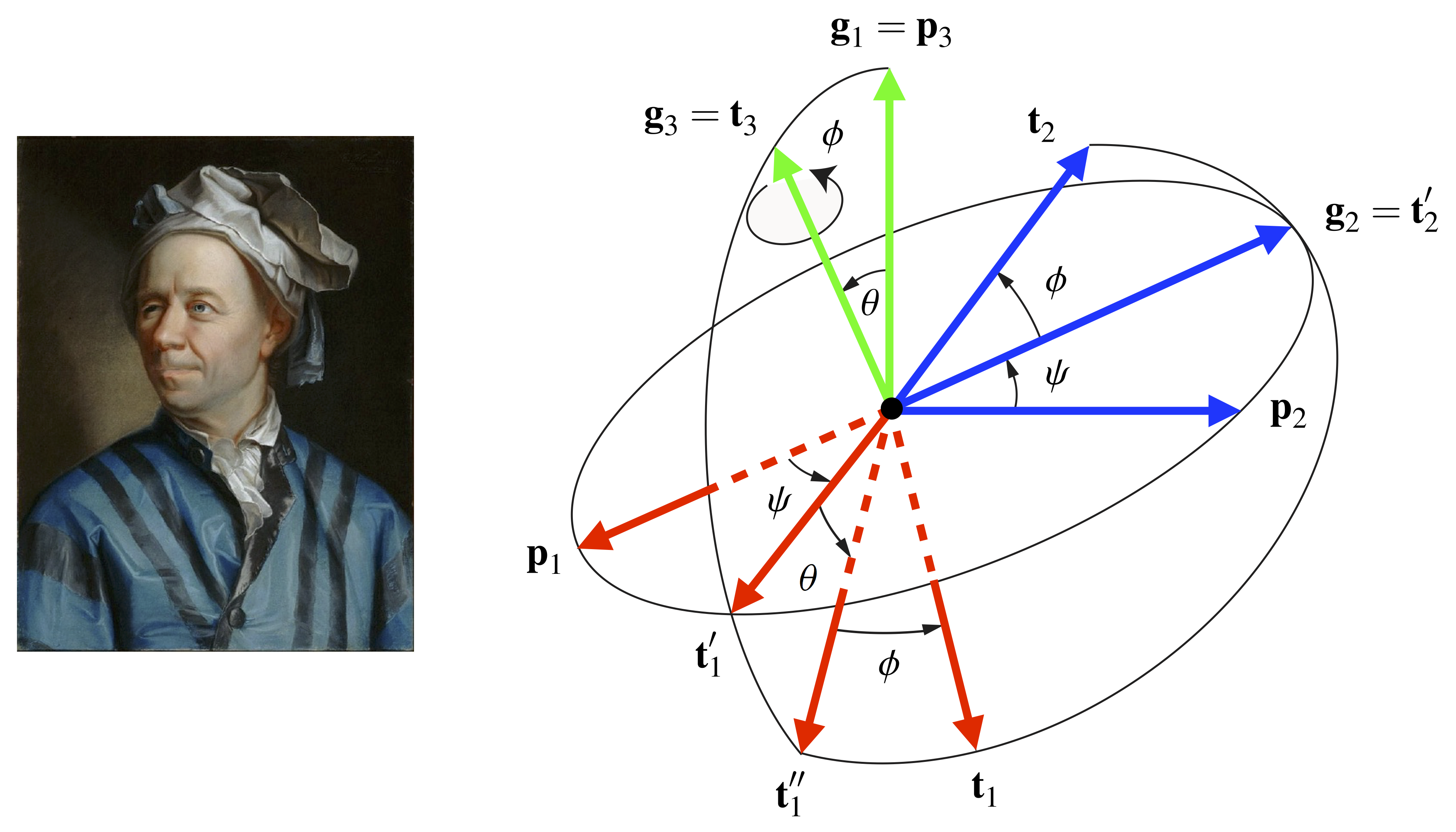
(3) $\begin{equation*} {\bf R} = {\bf L}\left(\phi, \, {\bf t}_3\right) {\bf L}\left(\theta, \, {\bf t}^{\prime}_2 \right) {\bf L}\left(\psi, \, {\bf p}_3\right). \end{equation*}$

**Figure 1.** Schematic of the 3-2-3 set of Euler angles and the individual rotations these angles represent. In this figure, the three Euler angles are denoted by $\psi = \gamma^1$ , $\theta = \gamma^2$ and $\phi = \gamma^3$ , and the rotation tensor ${\bf R}$ that they parameterize transforms the vectors ${\bf p}_i$ $(i = 1, \, 2, \, 3)$ to ${\bf t}_i$ . The image on the left is a portrait of Leonhard Euler.

While the Euler basis is composed of a set of unit vectors, the basis is typically non-orthogonal and, in many cases, not right-handed. This can be observed from the animation of the 3-2-3 Euler angle sequence provided in Figure 2, where the Euler basis is highlighted in cyan. Notice that the Euler basis vector ${\bf g}_2$ is perpendicular to the plane formed by ${\bf g}_1$ and ${\bf g}_3$ , i.e., ${\bf g}_2$ is perpendicular to both ${\bf g}_1$ and ${\bf g}_3$ .

**Figure 2.** Animation of the 3-2-3 Euler angle sequence. The fixed basis $\{{\bf p}_1, \, {\bf p}_2, \, {\bf p}_3\}$ is first rotated by $\psi = 0.3$ rad about ${\bf g}_1 = {\bf p}_3 = {\bf t}_3'$ ; the first intermediate basis $\{{\bf t}_1', \, {\bf t}_2', \, {\bf t}_3'\}$ is rotated by $\theta = 1$ rad about ${\bf g}_2 = {\bf t}_2' = {\bf t}_2''$ ; and the second intermediate basis $\{{\bf t}_1'', \, {\bf t}_2'', \, {\bf t}_3''\}$ is then rotated by $\phi = 0.7$ rad about ${\bf g}_3 = {\bf t}_3'' = {\bf t}_3$ to arrive at the corotational basis $\{{\bf t}_1, \, {\bf t}_2, \, {\bf t}_3\}$ .

The angular velocity vector

If we assume that the Euler basis vector ${\bf g}_1$ is constant, then the angular velocity vector associated with the Euler angle representation of a rotation tensor ${\bf R}$ can be established by using relative angular velocity vectors. In this case, there are two such vectors: $\hat{\bomega}_{{\bf L}\left(\gamma^2, \, {\bf g}_2\right)}$ and $\hat{\bomega}_{{\bf L}\left(\gamma^3, \, {\bf g}_3\right)}$ . For the first rotation, because its axis of rotation ${\bf g}_1$ is fixed, the angular velocity vector is simply

(4) $\begin{equation*} {\bomega}_{{\bf L}\left(\gamma^1, \, {\bf g}_1\right)} = \dot{\gamma}^1{\bf g}_1 . \end{equation*}$

The angular velocity of the second rotation relative to the first is

(5) $\begin{equation*} \hat{\bomega}_{{\bf L}\left(\gamma^2, \, {\bf g}_2\right)} = \dot{\gamma}^2{\bf g}_2, \end{equation*}$

while the angular velocity of the third rotation relative to the second is

(6) $\begin{equation*} \hat{\bomega}_{{\bf L}\left(\gamma^3, \, {\bf g}_3\right)} = \dot{\gamma}^3{\bf g}_3. \end{equation*}$

The calculation of the relative angular velocity vectors is similar to the example considered in our discussion of relative rotations and their angular velocities. Combining (4), (5), and (6), we conclude that the angular velocity vector associated with ${\bf R}$ is

(7) $\begin{eqnarray*} {\bomega}_{\bf R} \!\!\!\!\! &=& \!\!\!\!\! {\bomega}_{{\bf L}\left(\gamma^1, \, {\bf g}_1\right)} + \hat{\bomega}_{{\bf L}\left(\gamma^2, \, {\bf g}_2\right)} + \hat{\bomega}_{{\bf L}\left(\gamma^3, \, {\bf g}_3\right)} \\[0.075in] &=& \!\!\!\!\! \dot{\gamma}^1{\bf g}_1 + \dot{\gamma}^2{\bf g}_2 + \dot{\gamma}^3{\bf g}_3 . \end{eqnarray*}$

The simplicity of this representation is remarkable. If the rotation tensor ${\bf R}$ transforms the fixed vectors ${\bf p}_i$ into the corotational vectors ${\bf t}_i$ , then it is possible to express the Euler basis in terms of either set of vectors. Alternative approaches to establishing (7) can be found in various textbooks. In one such approach, all three Euler angles are considered to be infinitesimal. A good example of this approach can be found in Section 2.9 of Lurie’s text [8]. Another approach, which can be found in [9, 10] and dates to Euler, features spherical geometry. Finally, a third, but lengthy, approach involves differentiating the rotation tensor (1), computing the angular velocity tensor $\bOmega_{\bf R}$ , and then calculating its corresponding axial vector.

Singularities

For the Euler angles to effectively parameterize all rotations, we must assume that we can find $\gamma^i$ and $\dot{\gamma}^i$ such that (7) holds for any given angular velocity vector $\bomega_{\bf R}$ . For this to happen, it is necessary and sufficient that the Euler basis vectors ${\bf g}_1$ , ${\bf g}_2$ , and ${\bf g}_3$ span $\euclid^3$ . When these vectors are not linearly independent, we say that the Euler angles have a singularity. This singularity is unavoidable for Euler angles and occurs for certain values of $\gamma^2$ . Thus, it is necessary to restrict this angle to avoid these singularities. In the motion of a rigid body, the singularity manifests in the determinant of mass matrix $\mathsf{M}$ associated with the kinetic energy of the rigid body vanishing and $\mathsf{M}$ becoming non-invertible.

The Euler angle singularity is often erroneously referred to as “gimbal lock” (e.g., see [11]). However, as correctly pointed out by Mebius et al. [12] and discussed in further detail in Hemingway and O’Reilly [13], gimbal lock is a physical phenomenon where the application of moments and forces to a system of rigid bodies has no effect on the dynamics of the generalized coordinates of the system of rigid bodies. The illustration of gimbal lock often involves a body that is suspended by a pair of gimbals. For this system of three rigid bodies, gimbal lock occurs when the axes of relative rotation of one gimbal and the rotation of the suspended body relative to the other gimbal becoming parallel or antiparallel. As discussed in [13,14], it can be shown that gimbal lock does not lead to singularity of the mass matrix for the dynamics of the system of rigid bodies.

The dual Euler basis

For future developments, it is also convenient to define the dual Euler basis $\{{\bf g}^j\}$ $(j = 1, \, 2, \, 3)$ such that ${\bf g}^j\cdot{\bf g}_i = \delta^j_i$ , where $\delta^j_i$ is the Kronecker delta. The dual Euler basis vectors are analogous to the contravariant basis vectors in differential geometry and have similar uses in dynamics. We will use the dual Euler basis later when discussing particular sets of Euler angles; a rapid summary of this and other uses can be found in [14, 15, 16]. One method of determining the dual Euler basis is to express the Euler basis vectors ${\bf g}_i$ in terms of a right-handed basis, say, $\{ {\bf t}_i \}$ . Then, for example, to determine ${\bf g}^3$ , we could write ${\bf g}^3 = a{\bf t}_1 + b{\bf t}_2 + c {\bf t}_3$ and solve the three equations ${\bf g}_1\cdot{\bf g}^3 = 0$ , ${\bf g}_2\cdot{\bf g}^3 = 0$ , and ${\bf g}_3\cdot{\bf g}^3 = 1$ for the three unknowns $a$ , $b$ , and $c$ . Alternatively, one can use results from differential geometry [17]. Either way, the dual Euler basis vectors ${\bf g}^j$ are related to the Euler basis vectors ${\bf g}_i$ by

(8) $\begin{eqnarray*} && {\bf g}^1 = \frac{1}{g} \left({\bf g}_2\times{\bf g}_3\right), \\ \\[0.10in] && {\bf g}^2 = {\bf g}_2, \\ \\[0.10in] && {\bf g}^3 = \frac{1}{g} \left({\bf g}_1\times{\bf g}_2\right), \end{eqnarray*}$

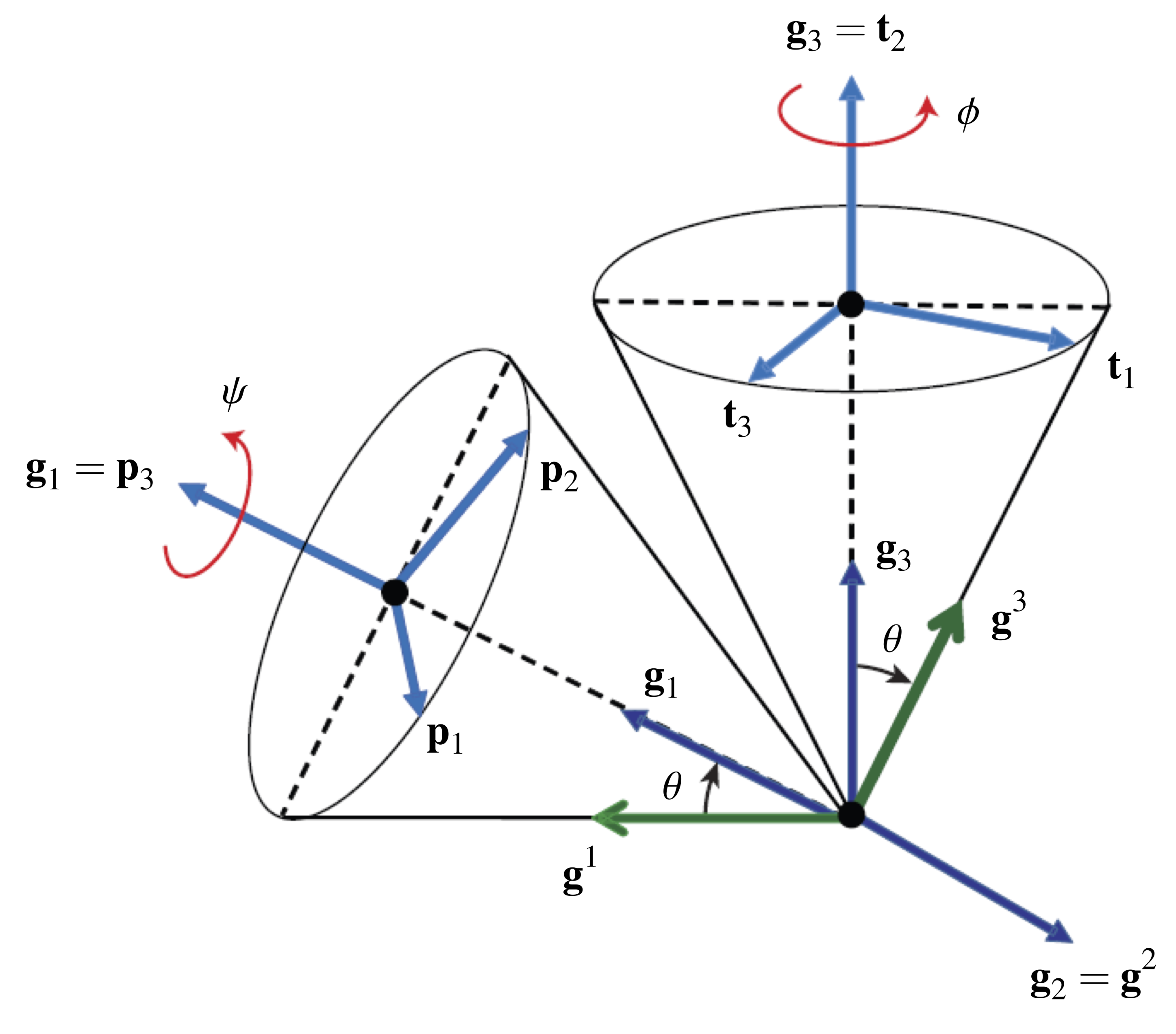
where $g = \left( {\bf g}_1\times{\bf g}_2\right)\cdot{\bf g}_3$ . These relationships are illustrated graphically in Figure 3 for a set of 3-1-2 Euler angles. Based on (8), we can make a few interesting observations: first, ${\bf g}^2 = {\bf g}_2$ , and thus $\lnorm {\bf g}^2 \rnorm = 1$ , for all possible sets of Euler angles; and second, $\lnorm {\bf g}^1 \rnorm$ and $\lnorm {\bf g}^3 \rnorm$ depend on $\gamma^2$ . When the Euler angles have singularities, one will find that the dual Euler basis vectors ${\bf g}^1$ and ${\bf g}^3$ cannot be defined.

**Figure 3.** Graphical representation of the Euler basis vectors and the dual Euler basis vectors for a set of 3-1-2 Euler angles. In this figure, $\psi = \gamma^1$ , $\theta = \gamma^2 > 0$ , and $\phi = \gamma^3$ .

The 3-2-1 set of Euler angles

To elaborate further on the Euler angles, we now consider the 3-2-1 set of Euler angles depicted in Figure 4. This set is arguably among the most popular sets of Euler angles. The 3-2-1 Euler angles are used in Greenwood’s text [18], Rao’s text [19], and numerous texts on vehicle and aircraft dynamics. In several communities, these angles are known as examples of the Tait [20] and/or Bryan [3] angles (after Peter G. Tait (1831-1901) and George H. Bryan (1864-1928)) or the Euler-Cardan angles (after Euler and Girolamo Cardano (1501-1576)).

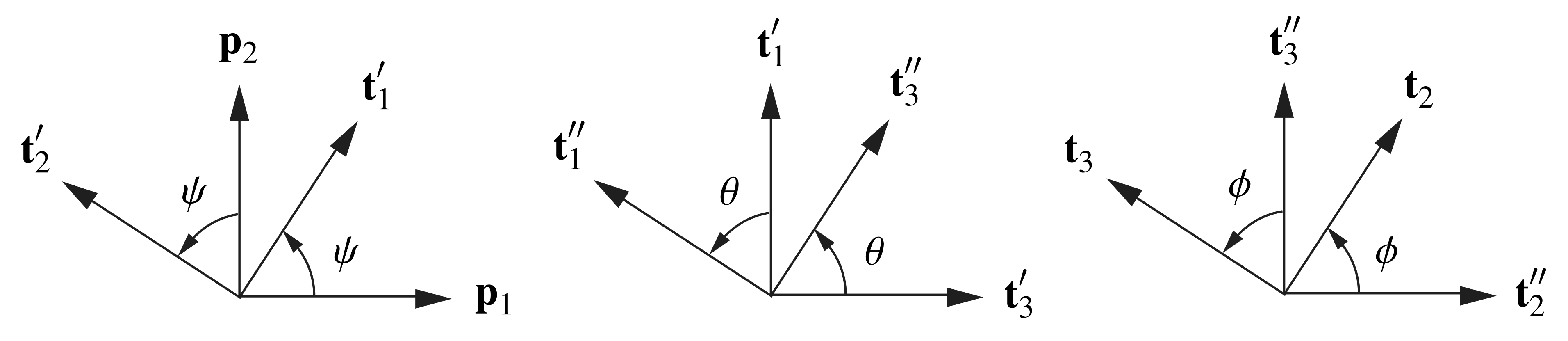
**Figure 4.** The transformations of various basis vectors induced by the individual angles in a set of 3-2-1 Euler angles.

Referring to Figure 4, suppose the corresponding rotation tensor has the representation

(9) $\begin{equation*} {\bf R} = \sum_{i \, \, = \, 1}^3 {\bf t}_i \otimes {\bf p}_i, \end{equation*}$

where $\{ {\bf p}_i \}$ is a fixed Cartesian basis. The first rotation transforms the vectors ${\bf p}_i$ to ${\bf t}^{\prime}_i$ through a rotation of $\psi$ about the axis ${\bf p}_3 = {\bf t}^{\prime}_3$ . In the second rotation, ${\bf t}^{\prime}_i$ are transformed into ${\bf t}^{\prime \prime}_i$ by a rotation $\theta$ about ${\bf t}^{\prime}_2 = {\bf t}^{\prime \prime}_2$ . The third and final rotation transforms ${\bf t}^{\prime \prime}_i$ to the corotational basis vectors ${\bf t}_i$ through a rotation of $\phi$ about the axis ${\bf t}^{\prime \prime}_1 = {\bf t}_1$ . Thus,

(10) $\begin{equation*} {\bf R} = \grave{\bf R}(\psi, \, \theta, \, \phi) = {\bf L}\left(\phi, \, {\bf t}_1\right){\bf L}\left(\theta, \, {\bf t}^{\prime}_2\right){\bf L}\left(\psi, \, {\bf p}_3\right) , \end{equation*}$

where

(11) $\begin{eqnarray*} && {\bf t}^{\prime}_i = {\bf L}\left(\psi, \, {\bf p}_3\right){\bf p}_i, \\ \\ && {\bf t}^{\prime \prime}_i = {\bf L}\left(\theta, \, {\bf t}^{\prime}_2\right){\bf t}^{\prime}_i, \\ \\ && {\bf t}_i = {\bf L}\left(\phi, \, {\bf t}_1\right){\bf t}^{\prime \prime}_i. \end{eqnarray*}$

It is not difficult to express the various basis vectors as linear combinations of each other:

(12) $\begin{eqnarray*} && \left[ \begin{array}{c} {\bf t}^{\prime}_1 \\ {\bf t}^{\prime}_2 \\ {\bf t}^{\prime}_3 \end{array} \right] = \left[ \begin{array}{c c c } \cos(\psi) & \sin(\psi) & 0 \\ - \sin(\psi) & \cos(\psi) & 0 \\ 0 & 0 & 1 \end{array} \right] \left[\begin{array}{c} {\bf p}_1 \\ {\bf p}_2 \\ {\bf p}_3 \end{array} \right], \\ \\ \\ && \left[ \begin{array}{c} {\bf t}^{\prime \prime}_1 \\ {\bf t}^{\prime \prime}_2 \\ {\bf t}^{\prime \prime}_3 \end{array} \right] = \left[ \begin{array}{c c c } \cos(\theta) & 0 & - \sin(\theta) \\ 0 & 1 & 0 \\ \sin(\theta) & 0 & \cos(\theta) \end{array} \right] \left[ \begin{array}{c} {\bf t}^{\prime}_1 \\ {\bf t}^{\prime}_2 \\ {\bf t}^{\prime}_3 \end{array} \right], \\ \\ \\ && \left[ \begin{array}{c} {\bf t}_1 \\ {\bf t}_2 \\ {\bf t}_3 \end{array} \right] = \left[ \begin{array}{c c c } 1 & 0 & 0 \\ 0 & \cos(\phi) & \sin(\phi) \\ 0 & - \sin(\phi) & \cos(\phi) \end{array} \right] \left[ \begin{array}{c} {\bf t}^{\prime \prime}_1 \\ {\bf t}^{\prime \prime}_2 \\ {\bf t}^{\prime \prime}_3 \end{array} \right]. \end{eqnarray*}$

The inverses of these relationships are easy to obtain because each of the three matrices in (12) is orthogonal. As the inverse of an orthogonal matrix is its transpose, we quickly arrive at the sought-after results:

(13) $\begin{eqnarray*} && \left[ \begin{array}{c} {\bf p}_1 \\ {\bf p}_2 \\ {\bf p}_3 \end{array} \right] = \left[ \begin{array}{c c c } \cos(\psi) & - \sin(\psi) & 0 \\ \sin(\psi) & \cos(\psi) & 0 \\ 0 & 0 & 1 \end{array} \right] \left[\begin{array}{c} {\bf t}^{\prime}_1 \\ {\bf t}^{\prime}_2 \\ {\bf t}^{\prime}_3 \end{array} \right], \\ \\ \\ && \left[ \begin{array}{c} {\bf t}^{\prime}_1 \\ {\bf t}^{\prime}_2 \\ {\bf t}^{\prime}_3 \end{array} \right] = \left[ \begin{array}{c c c } \cos(\theta) & 0 & \sin(\theta) \\ 0 & 1 & 0 \\ - \sin(\theta) & 0 & \cos(\theta) \end{array} \right] \left[ \begin{array}{c} {\bf t}^{\prime \prime}_1 \\ {\bf t}^{\prime \prime}_2 \\ {\bf t}^{\prime \prime}_3 \end{array} \right], \\ \\ \\ && \left[ \begin{array}{c} {\bf t}^{\prime \prime}_1 \\ {\bf t}^{\prime \prime}_2 \\ {\bf t}^{\prime \prime}_3 \end{array} \right] = \left[ \begin{array}{c c c } 1 & 0 & 0 \\ 0 & \cos(\phi) & - \sin(\phi) \\ 0 & \sin(\phi) & \cos(\phi) \end{array} \right] \left[ \begin{array}{c} {\bf t}_1 \\ {\bf t}_2 \\ {\bf t}_3 \end{array} \right]. \end{eqnarray*}$

Relationships (12) and (13) can be combined to express ${\bf t}_i$ in terms of ${\bf p}_k$ and vice versa. Later, they will also be used to establish representations for the Euler and dual Euler bases in terms of ${\bf p}_k$ and ${\bf t}_i$ . By using (13), we can obtain expressions for the rotation tensor components $R_{ij} = ({\bf R}{\bf p}_j) \cdot {\bf p}_i$ . These components are conveniently expressed in matrix form, $\left [ R_{ij} \right ]$ :

(14) $\begin{equation*} \left[ \begin{array}{c c c} R_{11} & R_{12} & R_{13} \\ R_{21} & R_{22} & R_{23} \\ R_{31} & R_{32} & R_{33} \\ \end{array} \right] = \left[ \begin{array}{c c c } \cos(\psi) & - \sin(\psi) & 0 \\ \sin(\psi) & \cos(\psi) & 0 \\ 0 & 0 & 1 \end{array} \right] \left[ \begin{array}{c c c } \cos(\theta) & 0 & \sin(\theta) \\ 0 & 1 & 0 \\ - \sin(\theta) & 0 & \cos(\theta) \end{array} \right] \left[ \begin{array}{c c c } 1 & 0 & 0 \\ 0 & \cos(\phi) & - \sin(\phi) \\ 0 & \sin(\phi) & \cos(\phi) \end{array} \right]. \hspace{1in} \scalebox{0.001}{\textrm{\textcolor{white}{.}}} \end{equation*}$

Representation (14) is the transpose of what one might naively expect. Indeed, it is useful to note that

(15) $\begin{eqnarray*} && \left[ \begin{array}{c} {\bf p}_1 \\ {\bf p}_2 \\ {\bf p}_3 \end{array} \right] = \left[ \begin{array}{c c c} R_{11} & R_{12} & R_{13} \\ R_{21} & R_{22} & R_{23} \\ R_{31} & R_{32} & R_{33} \\ \end{array} \right] \left[ \begin{array}{c} {\bf t}_1 \\ {\bf t}_2 \\ {\bf t}_3 \end{array} \right], \\ \\ \\ && \left[ \begin{array}{c} {\bf t}_1 \\ {\bf t}_2 \\ {\bf t}_3 \end{array} \right] = \left[ \begin{array}{c c c} R_{11} & R_{21} & R_{31} \\ R_{12} & R_{22} & R_{32} \\ R_{13} & R_{23} & R_{33} \\ \end{array} \right] \left[ \begin{array}{c} {\bf p}_1 \\ {\bf p}_2 \\ {\bf p}_3 \end{array} \right]. \end{eqnarray*}$

The Euler basis

By examining the individual rotations in (12), we can show that the Euler basis vectors have the equivalent representations

(16) $\begin{eqnarray*} \left[ \begin{array}{c} {\bf g}_1 \\ {\bf g}_2 \\ {\bf g}_3 \end{array} \right] = \left[ \begin{array}{c} {\bf p}_3 \\ {\bf t}^{\prime}_2 \\ {\bf t}_1 \end{array} \right] \!\!\!\!\! &=& \!\!\!\!\! \left[ \begin{array}{c c c } - \sin(\theta) & \sin(\phi)\cos(\theta) & \cos(\phi)\cos(\theta) \\ 0 & \cos(\phi) & - \sin(\phi) \\ 1 & 0 & 0 \end{array} \right] \left[\begin{array}{c} {\bf t}_1 \\ {\bf t}_2 \\ {\bf t}_3 \end{array} \right] \\ \\[0.10in] &=& \!\!\!\!\! \left[ \begin{array}{c c c } 0 & 0 & 1 \\ - \sin(\psi) & \cos(\psi) & 0 \\ \cos(\theta)\cos(\psi) & \cos(\theta)\sin(\psi) & -\sin(\theta) \end{array} \right] \left[\begin{array}{c} {\bf p}_1 \\ {\bf p}_2 \\ {\bf p}_3 \end{array} \right]. \hspace{1in} \scalebox{0.001}{\textrm{\textcolor{white}{.}}} \end{eqnarray*}$

The former representation is useful for establishing the angular velocity components $\bomega_{\bf R}\cdot{\bf t}_i$ , while the latter is helpful in obtaining $\bomega_{\bf R}\cdot{\bf p}_k$ .

The dual Euler basis

We can now determine the dual Euler basis vectors ${\bf g}^k$ . First, express each of the dual Euler basis vectors in terms of their components relative to, say, the corotational basis $\left\{{\bf t}_1, \, {\bf t}_2, \, {\bf t}_3\right\}$ :

(17) $\begin{equation*} {\bf g}^k = g^{k1}{\bf t}_1 + g^{k2}{\bf t}_2 + g^{k3}{\bf t}_3. \end{equation*}$

Combining these results in matrix-vector form,

(18) $\begin{equation*} \left[ \begin{array}{c} {\bf g}^1 \\ {\bf g}^2 \\ {\bf g}^3 \end{array} \right] = \left[ \begin{array}{c c c} g^{11} & g^{12} & g^{13} \\ g^{21} & g^{22} & g^{23} \\ g^{31} & g^{32} & g^{33} \end{array} \right] \left[\begin{array}{c} {\bf t}_1 \\ {\bf t}_2 \\ {\bf t}_3 \end{array} \right]. b \end{equation*}$

With the assistance of (16)₁, the relations ${\bf g}_i\cdot{\bf g}^k = \delta^k_i$ can be expressed as nine equations for the nine unknown components $g^{ik}$ :

(19) $\begin{equation*} \left[ \begin{array}{c c c } - \sin(\theta) & \sin(\phi)\cos(\theta) & \cos(\phi)\cos(\theta) \\ 0 & \cos(\phi) & - \sin(\phi) \\ 1 & 0 & 0 \end{array} \right] \left[ \begin{array}{c c c} g^{11} & g^{21} & g^{31} \\ g^{12} & g^{22} & g^{32} \\ g^{13} & g^{23} & g^{33} \end{array} \right] = \left[ \begin{array}{c c c } 1 & 0 & 0 \\ 0 & 1 & 0 \\ 0 & 0 & 1 \end{array} \right]. \hspace{1in} \scalebox{0.001}{\textrm{\textcolor{white}{.}}} \end{equation*}$

Isolating the matrix $\left[g^{ik}\right]$ on the left-hand side of this system of equations, we find that

(20) $\begin{equation*} \left[ \begin{array}{c c c} g^{11} & g^{12} & g^{13} \\ g^{21} & g^{22} & g^{23} \\ g^{31} & g^{32} & g^{33} \end{array} \right] = \left[ \begin{array}{c c c } 0 & \sin(\phi)\sec(\theta) & \cos(\phi)\sec(\theta) \\ 0 & \cos(\phi) & - \sin(\phi) \\ 1 & \sin(\phi)\tan(\theta) & \cos(\phi)\tan(\theta) \end{array} \right]. \hspace{1in} \scalebox{0.001}{\textrm{\textcolor{white}{.}}} \end{equation*}$

Therefore, the dual Euler basis vectors are given by

(21) $\begin{equation*} \left[ \begin{array}{c} {\bf g}^1 \\ {\bf g}^2 \\ {\bf g}^3 \end{array} \right] = \left[ \begin{array}{c c c } 0 & \sin(\phi)\sec(\theta) & \cos(\phi)\sec(\theta) \\ 0 & \cos(\phi) & - \sin(\phi) \\ 1 & \sin(\phi)\tan(\theta) & \cos(\phi)\tan(\theta) \end{array} \right] \left[\begin{array}{c} {\bf t}_1 \\ {\bf t}_2 \\ {\bf t}_3 \end{array} \right]. \end{equation*}$

If we had instead begun by expressing the dual Euler basis vectors in terms of components with respect to the fixed basis $\left\{{\bf p}_1, \, {\bf p}_2, \, {\bf p}_3\right\}$ , then we would have found the following representations:

(22) $\begin{equation*} \left[ \begin{array}{c} {\bf g}^1 \\ {\bf g}^2 \\ {\bf g}^3 \end{array} \right] = \left[ \begin{array}{c c c } \cos(\psi)\tan(\theta) & \sin(\psi)\tan(\theta) & 1 \\ - \sin(\psi) & \cos(\psi) & 0 \\ \cos(\psi)\sec(\theta) & \sin(\psi)\sec(\theta) & 0 \end{array} \right] \left[\begin{array}{c} {\bf p}_1 \\ {\bf p}_2 \\ {\bf p}_3 \end{array} \right]. \end{equation*}$

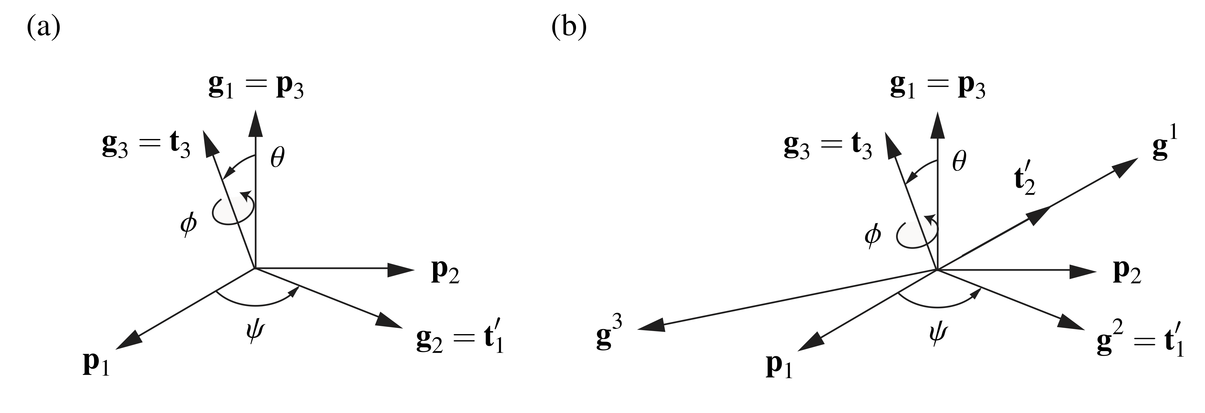
The dual Euler basis vectors are illustrated in Figure 5.

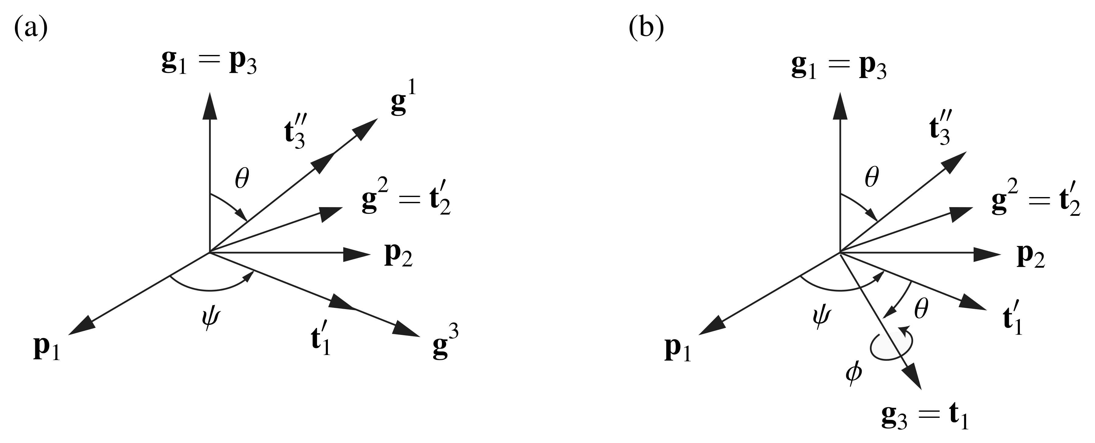
**Figure 5.** (a) The dual Euler basis vectors ${\bf g}^k$ for a 3-2-1 set of Euler angles: ${\bf g}^1 \parallel {\bf t}^{\prime \prime}_3$ , ${\bf g}^2 = {\bf t}^{\prime}_2$ , and ${\bf g}^3 \parallel {\bf t}^{\prime}_1$ . (b) The Euler angles $\psi$ and $\theta$ serve as coordinates for the Euler basis vector ${\bf g}_3 = {\bf t}_1$ in a manner that is similar to the role that spherical polar coordinates play in parameterizing the unit vectors ${\bf e}_R$ and ${\bf e}_\phi$ .

For completeness, we note that when $\theta \ne \pm \frac{\pi}{2}$ rad, one can also express the Euler basis vectors in terms of the dual Euler basis:

(23) $\begin{equation*} \left[ \begin{array}{c} {\bf g}_1 \\ {\bf g}_2 \\ {\bf g}_3 \end{array} \right] = \left[ \begin{array}{c c c } 1 & 0 & - \sin(\theta) \\ 0 & 1 & 0 \\ -\sin(\theta) & 0 & 1 \end{array} \right] \left[ \begin{array}{c} {\bf g}^1 \\ {\bf g}^2 \\ {\bf g}^3 \end{array} \right]. \end{equation*}$

The simplicity of this relationship (related versions of which hold for the other 11 sets of Euler angles) is surprising.

Singularities

If we examine (16), we see that the Euler basis fails to be a basis for $\euclid^3$ when $\theta = \pm \frac{\pi}{2}$ rad: ${\bf t}_1 = \pm {\bf p}_3$ , and thus the Euler basis does not span $\euclid^3$ . We can also infer this fact from Figure 5 if we consider the angles $\psi$ and $\theta + \frac{\pi}{2}$ to be spherical polar coordinates for ${\bf g}_3 = {\bf t}_1$ . To avoid this singularity, it is necessary to place restrictions on the second Euler angle: $\theta \in \left(-\frac{\pi}{2}, \, \frac{\pi}{2}\right)$ rad. The other two angles are free to range from $0$ to $2\pi$ rad.

Angular velocity vectors

The angular velocity vector $\bomega_{\bf R}$ associated with the 3-2-1 Euler angles has several representations:

(24) $\begin{eqnarray*} \bomega_{\bf R} = - \frac{1}{2} \bepsilon \left[\dot{\bf R}{\bf R}^T\right] \!\!\!\!\! &=& \!\!\!\!\! \sum_{i \, \, = \, 1}^3 \dot{\gamma}^i {\bf g}_i \\ \\ &=& \!\!\!\!\! \dot{\psi}{\bf p}_3 + \dot{\theta}{\bf t}^{\prime}_2 + \dot{\phi}{\bf t}_1 \\[0.075in] &=& \!\!\!\!\! (- \dot{\psi} \sin(\theta) + \dot{\phi}){\bf t}_1 + (\dot{\psi}\sin(\phi)\cos(\theta) + \dot{\theta}\cos(\phi)){\bf t}_2 + (\dot{\psi}\cos(\phi)\cos(\theta) - \dot{\theta}\sin(\phi)){\bf t}_3. \hspace{1in} \scalebox{0.001}{\textrm{\textcolor{white}{.}}} \end{eqnarray*}$

To arrive at the primitive representation $\bomega_{\bf R} = \dot{\psi}{\bf p}_3 + \dot{\theta}{\bf t}^{\prime}_2 + \dot{\phi}{\bf t}_1$ , we needed to compute two relative angular velocity vectors. We calculated the first of these, $\dot{\theta}{\bf t}^{\prime}_2$ , assuming ${\bf t}^{\prime}_i$ were fixed, and the second relative angular velocity vector, $\dot{\phi}{\bf t}_1$ , was computed by fixing ${\bf t}^{\prime \prime}_i$ . It is also interesting to note that the angular velocity vector $\bomega_{0_{\bf R}}$ has the representations

(25) $\begin{eqnarray*} \bomega_{0_{\bf R}} = - \frac{1}{2}\bepsilon\left[{\bf R}^T\dot{\bf R}\right] \!\!\!\!\! &=& \!\!\!\!\! {\bf R}^T{\bomega}_{\bf R} \\[0.05in] &=& \!\!\!\!\! \dot{\psi}{\bf R}^T{\bf p}_3 + \dot{\theta}{\bf R}^T{\bf t}^{\prime}_2 + \dot{\phi}{\bf R}^T{\bf t}_1 \\[0.075in] &=& \!\!\!\!\! (- \dot{\psi} \sin(\theta) + \dot{\phi}){\bf p}_1 + (\dot{\psi}\sin(\phi)\cos(\theta) + \dot{\theta}\cos(\phi)){\bf p}_2 + (\dot{\psi}\cos(\phi)\cos(\theta) - \dot{\theta}\sin(\phi)){\bf p}_3. \hspace{1in} \scalebox{0.001}{\textrm{\textcolor{white}{.}}} \end{eqnarray*}$

In establishing this result, we used the fact that ${\bf R}^T{\bf t}_i = {\bf p}_i$ . Lastly, we note that

(26) $\begin{eqnarray*} && \dot{\psi} = \bomega_{\bf R} \cdot{\bf g}^1, \\ \\ && \dot{\theta} = \bomega_{\bf R} \cdot{\bf g}^2, \\ \\ && \dot{\phi} = \bomega_{\bf R} \cdot{\bf g}^3. \end{eqnarray*}$

Using (21) to express the dual Euler basis vectors ${\bf g}^i$ in terms of their components relative to ${\bf t}_i$ , we find

(27) $\begin{equation*} \left[ \begin{array}{c} \dot{\psi} \\ \dot{\theta} \\ \dot{\phi} \end{array} \right] = \left[ \begin{array}{c c c } 0 & \sin(\phi)\sec(\theta) & \cos(\phi)\sec(\theta) \\ 0 & \cos(\phi) & - \sin(\phi) \\ 1 & \sin(\phi)\tan(\theta) & \cos(\phi)\tan(\theta) \end{array} \right] \left[\begin{array}{c} \omega_1 \\ \omega_2 \\ \omega_3 \end{array} \right], \hspace{1in} \scalebox{0.001}{\textrm{\textcolor{white}{.}}} \end{equation*}$

where $\omega_i = \bomega_{\bf R} \cdot{\bf t}_i$ are the corotational components of angular velocity. Suppose the initial orientation of a body is described by $\psi\left(t_0\right)$ , $\theta\left(t_0\right)$ , and $\phi\left(t_0\right)$ , or, equivalently, ${\bf R}\left(t_0\right)$ . Given measurements for $\omega_i(t)$ , the differential equations in (27) can be numerically integrated to determine the body’s orientation over time, ${\bf R}(t)$ . This idea forms the foundation of inertial navigation.

The 3-1-3 set of Euler angles

We now discuss another popular set of Euler angles: the 3-1-3 Euler angles. These angles, which are illustrated in Figure 6, are the angles Lagrange used¹, and they were also used by Arnol’d [21], Landau and Lifshitz [22], and Thomson [23], among many others. For motions of a spinning top, the 3-1-3 Euler angles are identified with precession, nutation, and spin, respectively.

**Figure 6.** The transformations of various basis vectors induced by the individual angles in a set of 3-1-3 Euler angles.

Paralleling the developments for the 3-2-1 Euler angles, we represent a rotation tensor ${\bf R}$ as the product of three rotations:

(28) $\begin{equation*} {\bf R} = {\bf L}\left(\phi, \, {\bf t}_3 \right) {\bf L}\left(\theta, \, {\bf t}^{\prime}_1\right){\bf L}\left(\psi, \, {\bf p}_3\right), \end{equation*}$

where $\{ {\bf p}_3, \, {\bf t}^{\prime}_1, \, {\bf t}_3 \}$ is the Euler basis, and

(29) $\begin{eqnarray*} && {\bf t}^{\prime}_i = {\bf L}\left(\psi, \, {\bf p}_3\right){\bf p}_i, \\ \\ && {\bf t}^{\prime \prime}_i = {\bf L}\left(\theta, \, {\bf t}^{\prime}_1\right){\bf t}'_i, \\ \\ && {\bf t}_i = {\bf L}\left(\phi, \, {\bf t}_3\right){\bf t}^{\prime \prime}_i. \end{eqnarray*}$

Note that we are using the same notation for the three Euler angles as we did for the 3-2-1 set. However, it should be clear that $\theta$ and $\phi$ represent different angles of rotation for these two distinct sets of Euler angles. Finally, harking back to many of the celestial mechanics applications for the 3-1-3 set of Euler angles, we wish to mention that the line passing through the origin that is parallel to ${\bf t}^{\prime}_1$ is often known as the line of nodes [23].

The Euler basis

After expressing ${\bf p}_3$ , ${\bf t}^{\prime}_1$ , and ${\bf t}_3$ in terms of ${\bf t}_i$ and ${\bf p}_k$ , it is not difficult to show that the Euler basis $\{ {\bf g}_j \}$ has the representations

(30) $\begin{eqnarray*} \left[ \begin{array}{c} {\bf g}_1 \\ {\bf g}_2 \\ {\bf g}_3 \end{array} \right] = \left[ \begin{array}{c} {\bf p}_3 \\ {\bf t}^{\prime}_1 \\ {\bf t}_3 \end{array} \right] \!\!\!\!\! &=& \!\!\!\!\! \left[ \begin{array}{c c c } \sin(\phi)\sin(\theta) & \cos(\phi)\sin(\theta) & \cos(\theta) \\ \cos(\phi) & - \sin(\phi) & 0 \\ 0 & 0 & 1 \end{array} \right] \left[\begin{array}{c} {\bf t}_1 \\ {\bf t}_2 \\ {\bf t}_3 \end{array} \right] \\ \\[0.10in] &=& \!\!\!\!\! \left[ \begin{array}{c c c } 0 & 0 & 1 \\ \cos(\psi) & \sin(\psi) & 0 \\ \sin(\theta)\sin(\psi) & -\sin(\theta)\cos(\psi) & \cos(\theta) \end{array} \right] \left[\begin{array}{c} {\bf p}_1 \\ {\bf p}_2 \\ {\bf p}_3 \end{array} \right]. \hspace{1in} \scalebox{0.001}{\textrm{\textcolor{white}{.}}} \end{eqnarray*}$

The dual Euler basis

By following the procedure that led to the dual Euler basis of the 3-2-1 Euler angles or by using the identities in (8), we find that the dual Euler basis $\left\{ {\bf g}^i \right\}$ for a 3-1-3 set has the representations

(31) $\begin{eqnarray*} \left[ \begin{array}{c} {\bf g}^1 \\ {\bf g}^2 \\ {\bf g}^3 \end{array} \right] \!\!\!\!\! &=& \!\!\!\!\! \left[ \begin{array}{c c c } \sin(\phi)\mbox{cosec}(\theta) & \cos(\phi)\mbox{cosec}(\theta) & 0 \\ \cos(\phi) & - \sin(\phi) & 0 \\ - \sin(\phi)\cot(\theta) & - \cos(\phi)\cot(\theta) & 1 \end{array} \right] \left[\begin{array}{c} {\bf t}_1 \\ {\bf t}_2 \\ {\bf t}_3 \end{array} \right] \\ \\[0.10in] &=& \!\!\!\!\! \left[ \begin{array}{c c c } - \sin(\psi)\mbox{cot}(\theta) & \cos(\psi)\mbox{cot}(\theta) & 1 \\ \cos(\psi) & \sin(\psi) & 0 \\ \sin(\psi)\mbox{cosec}(\theta) & - \cos(\psi)\mbox{cosec}(\theta) & 0 \end{array} \right] \left[\begin{array}{c} {\bf p}_1 \\ {\bf p}_2 \\ {\bf p}_3 \end{array} \right]. \hspace{1in} \scalebox{0.001}{\textrm{\textcolor{white}{.}}} \end{eqnarray*}$

Consequently, we can also establish the result

(32) $\begin{equation*} \left[ \begin{array}{c} {\bf g}_1 \\ {\bf g}_2 \\ {\bf g}_3 \end{array} \right] = \left[ \begin{array}{c c c } 1 & 0 & \cos(\theta) \\ 0 & 1 & 0 \\ \cos(\theta) & 0 & 1 \end{array} \right] \left[ \begin{array}{c} {\bf g}^1 \\ {\bf g}^2 \\ {\bf g}^3 \end{array} \right] \end{equation*}$

for $\theta \ne 0, \, \pi$ rad. Both the Euler and dual Euler bases vectors are depicted in Figure 7.

**Figure 7.** (a) The Euler basis vectors and (b) the dual Euler basis vectors for the 3-1-3 set of Euler angles, where ${\bf g}^1 \parallel {\bf t}^{\prime}_2$ , ${\bf g}^2 = {\bf t}^{\prime}_1$ , and ${\bf g}^3 \parallel {\bf t}^{\prime \prime}_2$ .

Singularities

As with all sets of Euler angles, the 3-1-3 Euler angles are subject to restrictions. For a 3-1-3 set, the Euler basis fails to be a basis when $\theta = 0, \, \pi$ rad. This singularity is easy to see from (30) and Figure 7(a): ${\bf t}_3 = \pm {\bf p}_3$ in this case. As a result, the second Euler angle is restricted to $\theta \in (0, \, \pi)$ rad, while the other two angles are free to range from 0 to $2 \pi$ rad. Note the difference in range of $\theta$ for a 3-1-3 set compared to the 3-2-1 Euler angles.

The angular velocity vector

With the help of the expressions for the Euler basis vectors from (30), we can obtain representations for the angular velocity vector $\bomega_{\bf R}$ featuring the fixed basis $\left\{ {\bf p}_1, \, {\bf p}_2, \, {\bf p}_3\right\}$ and the corotational basis $\left\{ {\bf t}_1, \, {\bf t}_2, \, {\bf t}_3\right\}$ :

(33) $\begin{eqnarray*} \bomega_{\bf R} \!\!\!\!\! &=& \!\!\!\!\! \dot{\psi}{\bf p}_3 + \dot{\theta}{\bf t}^{\prime}_1 + \dot{\phi}{\bf t}_3 \\[0.075in] &=& \!\!\!\!\! (\dot{\phi}\sin(\psi)\sin(\theta) + \dot{\theta}\cos(\psi)){\bf p}_1 + (-\dot{\phi}\cos(\psi)\sin(\theta) + \dot{\theta}\sin(\psi)){\bf p}_2 + (\dot{\phi} \cos(\theta) + \dot{\psi}){\bf p}_3 \hspace{1in} \scalebox{0.001}{\textrm{\textcolor{white}{.}}} \\[0.075in] &=& \!\!\!\!\! (\dot{\psi}\sin(\phi)\sin(\theta) + \dot{\theta}\cos(\phi)){\bf t}_1 + (\dot{\psi}\cos(\phi)\sin(\theta) - \dot{\theta}\sin(\phi)){\bf t}_2 + (\dot{\psi} \cos(\theta) + \dot{\phi}){\bf t}_3 . \end{eqnarray*}$

As in the case of the 3-2-1 Euler angles, we can use the dual Euler basis vectors to relate the angular rates $\dot \psi$ , $\dot \theta$ , and $\dot \phi$ to the corotational components of the angular velocity vector, $\omega_i = \bomega_{\bf R} \cdot{\bf t}_i$ . Using (26) and (31)₁, for the 3-1-3 Euler angles,

(34) $\begin{equation*} \left[ \begin{array}{c} \dot{\psi} \\ \dot{\theta} \\ \dot{\phi} \end{array} \right] = \left[ \begin{array}{c c c } \sin(\phi)\mbox{cosec}(\theta) & \cos(\phi)\mbox{cosec}(\theta) & 0 \\ \cos(\phi) & - \sin(\phi) & 0 \\ - \sin(\phi)\cot(\theta) & - \cos(\phi)\cot(\theta) & 1 \end{array} \right] \left[\begin{array}{c} \omega_1 \\ \omega_2 \\ \omega_3 \end{array} \right]. \hspace{1in} \scalebox{0.001}{\textrm{\textcolor{white}{.}}} \end{equation*}$

Provided a body’s initial orientation and data for $\omega_i(t)$ , we can compute the body’s orientation over time by numerically integrating the system of differential equations in (34).

Other sets of Euler angles

For the Euler basis, one has three choices for ${\bf g}_1$ and, because ${\bf g}_1 \ne {\bf g}_2$ , two choices for ${\bf g}_2$ . Finally, there are two choices of ${\bf g}_3$ . Consequently, there are $3 \times 2 \times 2 = 12$ choices of the vectors for the Euler basis, and hence 12 sets of Euler angles. The easiest method to determine which set of Euler angles is being used is to specify the angular velocity vector $\bomega_{\bf R}$ . Here, expressions are given for each of the 12 sets of Euler angles for a rotation tensor ${\bf R} = \sum_{i \, \, = \, 1}^3 {\bf t}_i\otimes{\bf p}_i$ :

(35) $\begin{eqnarray*} && \mbox{1-2-3 set:} \quad {\bomega}_{\bf R} = \dot{\psi}{\bf p}_1 + \dot{\theta}{\bf t}^{\prime}_2 + \dot{\phi} {\bf t}_3, \\[0.075in] && \mbox{3-2-3 set:} \quad {\bomega}_{\bf R} = \dot{\psi}{\bf p}_3 + \dot{\theta}{\bf t}^{\prime}_2 + \dot{\phi} {\bf t}_3, \\[0.075in] && \mbox{1-2-1 set:} \quad {\bomega}_{\bf R} = \dot{\psi}{\bf p}_1 + \dot{\theta}{\bf t}^{\prime}_2 + \dot{\phi} {\bf t}_1, \\[0.075in] && \mbox{1-3-1 set:} \quad {\bomega}_{\bf R} = \dot{\psi}{\bf p}_1 + \dot{\theta}{\bf t}^{\prime}_3 + \dot{\phi} {\bf t}_1, \\[0.075in] && \mbox{1-3-2 set:} \quad {\bomega}_{\bf R} = \dot{\psi}{\bf p}_1 + \dot{\theta}{\bf t}^{\prime}_3 + \dot{\phi} {\bf t}_2, \\[0.075in] && \mbox{2-3-1 set:} \quad {\bomega}_{\bf R} = \dot{\psi}{\bf p}_2 + \dot{\theta}{\bf t}^{\prime}_3 + \dot{\phi} {\bf t}_1, \\[0.075in] && \mbox{2-3-2 set:} \quad {\bomega}_{\bf R} = \dot{\psi}{\bf p}_2 + \dot{\theta}{\bf t}^{\prime}_3 + \dot{\phi} {\bf t}_2, \\[0.075in] && \mbox{2-1-2 set:} \quad {\bomega}_{\bf R} = \dot{\psi}{\bf p}_2 + \dot{\theta}{\bf t}^{\prime}_1 + \dot{\phi} {\bf t}_2, \\[0.075in] && \mbox{2-1-3 set:} \quad {\bomega}_{\bf R} = \dot{\psi}{\bf p}_2 + \dot{\theta}{\bf t}^{\prime}_1 + \dot{\phi} {\bf t}_3, \\[0.075in] && \mbox{3-1-3 set:} \quad {\bomega}_{\bf R} = \dot{\psi}{\bf p}_3 + \dot{\theta}{\bf t}^{\prime}_1 + \dot{\phi} {\bf t}_3, \\[0.075in] && \mbox{2-3-1 set:} \quad {\bomega}_{\bf R} = \dot{\psi}{\bf p}_2 + \dot{\theta}{\bf t}^{\prime}_3 + \dot{\phi} {\bf t}_1, \\[0.075in] && \mbox{3-1-2 set:} \quad {\bomega}_{\bf R} = \dot{\psi}{\bf p}_3 + \dot{\theta}{\bf t}^{\prime}_1 + \dot{\phi} {\bf t}_2. \end{eqnarray*}$

Notice how easy it is to describe which set of Euler angles is being used to parameterize a rotation ${\bf R}$ by simply writing down the corresponding representation for the angular velocity vector.

Bryan angles, Cardan angles, Tait angles, asymmetric sets, and symmetric sets

The 1-2-1, 1-3-1, 2-3-2, 2-1-2, 3-1-3, and 3-2-3 sets of Euler angles are known as the symmetric sets, whereas the other six sets are known as asymmetric sets. The latter sets are also known as the Cardan angles, Tait angles, or Bryan angles. Tait’s original discussion (of what we would call 1-2-3 Euler angles) can be seen in Section 12 of his 1868 paper [20]. In his seminal text [3] on aircraft stability that was published in 1911, Bryan introduced what we would refer to as a 2-3-1 set of Euler angles (see Figure 8). It is interesting to recall that the Wright brothers’ first successful flight was in 1903.

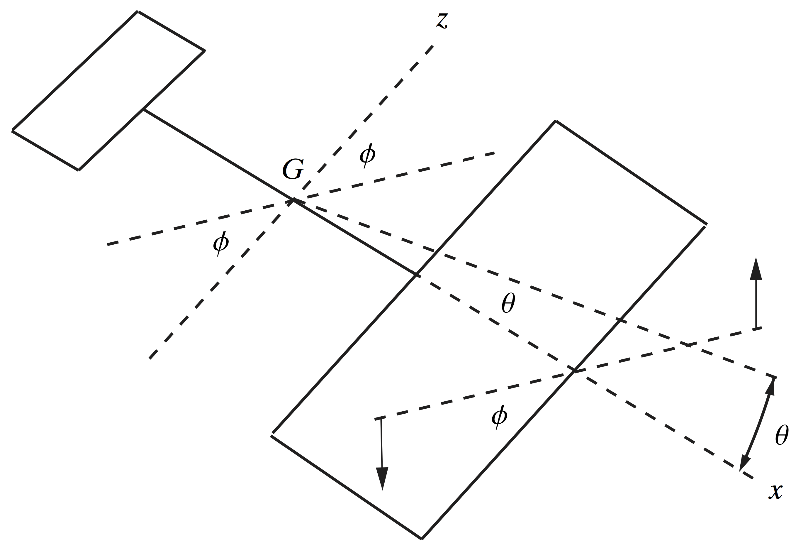**Figure 8.** Reproduction of Figure 3 in Bryan’s seminal text [3] on the stability of aircraft. The angles $\theta$ and $\phi$ in this figure are the aircrafts’ pitch and roll angles, respectively. The point $G$ is the center of mass of the aircraft, and $x$ and $z$ label the aircraft’s corotational axes.

Singularities

For all sets of Euler angles, a singularity is present for certain values of the second angle $\theta$ . At these values, the Euler basis fails to be a basis for $\euclid^3$ because ${\bf g}_1 = \pm {\bf g}_3$ . To avoid these singularities, it is often necessary to use two different sets of Euler angles and switch from one set to the other as a singularity is approached.

As mentioned earlier, it is a mistake to confuse gimbal lock with the singularities in the Euler angles. The former is a physical phenomenon while the latter is a mathematical phenomenon. For further details on this distinction, the reader is referred to the recent paper by Hemingway and O’Reilly [13].

Body angles and space angles

In the works of Kane et al. [24], six sets of body-three orientation angles, six sets of body-two orientation angles, six sets of space-three orientation angles, and six sets of space-two orientation angles are discussed. Each of these 24 parameterizations of a rotation can be shown to be equivalent to one of the 12 sets of Euler angles discussed above. Specifically, a set of body-three 3-2-1 orientation angles parameterizing a rotation tensor ${\bf R}$ is equivalent to a set of 3-2-1 Euler angles parameterizing ${\bf R}$ :

(36) $\begin{equation*} {\bf R} = {\bf L}\left(\phi, \, {\bf t}_1\right){\bf L}\left(\theta, \, {\bf t}^{\prime}_2\right){\bf L}\left(\psi, \, {\bf p}_3\right). \end{equation*}$

Similarly, a set of body-two 3-2-3 orientation angles parameterizing ${\bf R}$ is equivalent to a set of 3-2-3 Euler angles:

(37) $\begin{equation*} {\bf R} = {\bf L}\left(\phi, \, {\bf t}_3\right){\bf L}\left(\theta, \, {\bf t}^{\prime}_2\right){\bf L}\left(\psi, \, {\bf p}_3\right). \end{equation*}$

On the other hand, a set of space-three 3-2-1 orientation angles parameterizing ${\bf R}$ is equivalent to a set of 1-2-3 Euler angles:

(38) $\begin{equation*} {\bf R} = {\bf L}\left(\phi, \, {\bf t}_3\right){\bf L}\left(\theta, \, {\bf t}^{\prime}_2\right){\bf L}\left(\psi, \, {\bf p}_1\right). \end{equation*}$

Similarly, a set of space-two 3-1-3 orientation angles parameterizing ${\bf R}$ is equivalent to a set of 3-1-3 Euler angles:

(39) $\begin{equation*} {\bf R} = {\bf L}\left(\phi, \, {\bf t}_3\right){\bf L}\left(\theta, \, {\bf t}^{\prime}_1\right){\bf L}\left(\psi, \, {\bf p}_3\right). \end{equation*}$

Clearly, the primary distinction between a body-three 3-2-1 set (36) and a space-three 3-2-1 set (38) is in the order of the rotation axes.

With regard to the orientation angles and Euler angles, we mention here the work of Savransky and Kasdin [25], who demonstrated a way of extracting each of the six sets of body-three orientation angles, six sets of body-two orientation angles, six sets of space-three orientation angles, and six sets of space-two orientation angles from a matrix $\mathsf{R}$ . Savransky’s MATLAB code provides a wonderful illustration of these results by allowing the user to animate the same rotation using any of the aforementioned sets of angles. Based on the correspondences discussed above, the animation of, say, a body-three 1-2-3 set of orientation angles or a space-three 3-2-1 set of orientation angles is the same as for a set of 1-2-3 Euler angles.

Notes

See [1] and Section IX of the Second Part of [2]: Lagrange’s $\psi$ , $\omega$ , and $\phi$ correspond to our $\psi$ , $\theta$ , and $\phi$ , respectively.

Downloads

The MATLAB code used to generate the animation in Figure 2 is available here. This code animates any one of the 12 sequences of Euler angles by having the user provide the particular set and angular displacements of interest. A similar, but far more sophisticated, MATLAB code written by Dmitry Savransky can be downloaded from here.

References

Lagrange, J. L., Théorie de la libration de la Lune, et des autres phénomènes qui dépendent de la ﬁgure non sphèrique de cette Planète, Nouveaux Mémoires de l’Académie Royale des Sciences et des Belles-Lettres de Berlin 30 203–309 (1780-1782). Reprinted in pp. 5–122 of Oeuvres de Lagrange, Vol. 5, Gauthier-Villars, Paris (1870). Edited by J.-A. Serret.
Lagrange, J. L., Mécanique Analytique, in: J.-A. Serret, G. Darboux (eds.), Joseph Louis de Lagrange Oeuvres, Vol. 11/12, 4th ed., Georg Olms Verlag, Heidelberg (1973).
Bryan, G. H., Stability in Aviation: An Introduction to Dynamical Stability as Applied to the Motion of Aeroplanes, Macmillan, London (1911).
Cheng, H., and Gupta, K. C., An historical note on finite rotations, ASME Journal of Applied Mechanics 56(1) 139–145 (1989).
Wilson, C., D’Alembert versus Euler on the precession of the equinoxes and the mechanics of rigid bodies, Archive for History of Exact Sciences 37(3) 233–273 (1987).
Euler, L., Du mouvement d’un corps solides quelconque lorsqu’il tourne autour d’un axe mobile, Mémoires de l’Académie des Sciences der Berlin 16 176–227 (1760). The title translates to “On the motion of a solid body while it rotates about a moving axis.” Reprinted in pp. 313–356 of Euler, L., Leonhardi Euleri Opera Omnia, II, Vol. 8, Orell Füssli, Zürich (1965). Edited by C. Blanc.
Euler, L., De motu corporum circa punctum ﬁxum mobilum, in: Euler, L., Leonhardi Euleri Opera Postuma, Vol. 2, pp. 43–62, Orell Füssli, Zürich (1862). Reprinted in pp. 413–441 of Euler, L., Leonhardi Euleri Opera Omnia, II, Vol. 9, Orell Füssli, Zürich (1968). Edited by C. Blanc.
Lurie, A. I., Analytical Mechanics, Springer-Verlag, New York (2002). Translated from the Russian by A. Belyaev.
Kelvin, L., and Tait, P. G., Treatise on Natural Philosophy, reprinted ed., Cambridge University Press, Cambridge (1912).
Routh, E. J., The Elementary Part of a Treatise on the Dynamics of a System of Rigid Bodies, 7th ed., Macmillan, London (1905).
Shuster, M. D., A survey of attitude representations, Journal of the Astronautical Sciences 41(4) 439–517 (1993).
Mebius, J. E., Kasperink, H. R., and Kooijman, M. D., Mathematics for simulation of near-vertical aircraft attitudes, Making It Real: Proceedings CEAS Symposium on Simulation Technology, Delft, The Netherlands, Confederation of European Aerospace Societies, Paper Number MOD04, 241–-246 (1995).
Hemingway, E. G. and O’Reilly, O. M., Perspectives on Euler angle singularities, gimbal lock, and the orthogonality of applied forces and applied moments, Multibody System Dynamics 44(1) 31-56 (2018).
O’Reilly, O. M., Intermediate Dynamics for Engineers: Newton-Euler and Lagrangian Mechanics, 2nd ed., Cambridge University Press, Cambridge (2020).
O’Reilly, O. M., The dual Euler basis: Constraints, potentials, and Lagrange’s equations in rigid body dynamics, ASME Journal of Applied Mechanics 74(2) 256–258 (2007).
O’Reilly, O. M., Intermediate Dynamics for Engineers: A Unified Treatment of Newton-Euler and Lagrangian Mechanics, Cambridge University Press, Cambridge (2008).
Simmonds, J. G., A Brief on Tensor Analysis, 2nd ed., Springer-Verlag, New York (1994).
Greenwood, D. T., Principles of Dynamics, 2nd ed., Prentice Hall, Englewood Cliffs, NJ (1988).
Rao, A. V., Dynamics of Particles and Rigid Bodies: A Systematic Approach, Cambridge University Press, Cambridge (2006).
Tait, P. G., On the rotation of a rigid body about a fixed point, Proceedings of the Royal Society of Edinburgh 25(2) 261-303 (1869). Reprinted in pp. 86–127 of Tait, P. G., Scientific Papers, Vol. 1, Cambridge University Press, Cambridge (1898).
Arnol’d, V. I., Mathematical Methods of Classical Mechanics, 2nd ed., Springer-Verlag, New York (1989). Translated from the Russian by K. Vogtmann and A. Weinstein.
Landau, L. D., and Lifshitz, E. M., Mechanics, Vol. 1, 3rd ed., Butterworth-Heinenann, Oxford and Boston (1976). Translated from the Russian by J. B. Sykes and J. S. Bell.
Thomson, W. T., Introduction to Space Dynamics, Dover Publications, New York (1986). Reprint of the John Wiley & Sons, Inc., New York, 1963 edition.
Kane, T. R., Likins, P. W., and Levinson, D. A., Spacecraft Dynamics, McGraw-Hill, New York (1983).
Savransky, D., and Kasdin, N. J., An efficient method for extracting Euler angles from direction cosine matrices, unpublished notes (2013).