

Predicting panel attrition using multiple operationalisations of response time
Minderop, I. (2023). Predicting panel attrition using multiple operationalisations of response time. Survey Methods: Insights from the Field. Retrieved from https://surveyinsights.org/?p=18304
© the authors 2023. This work is licensed under a Creative Commons Attribution 4.0 International License (CC BY 4.0) 
Abstract
Panel attrition is a major problem for panel survey infrastructures. When panelists attrit from a panel survey, the infrastructure is faced with (i) the costs of recruiting new respondents, (ii) a broken timeline of existing data, and (iii) potential nonresponse bias. Previous studies have shown that panel attrition can be predicted using respondents’ response time. However, response time has been operationalised in multiple ways, such as (i) the number of days it takes respondents to participate, (ii) the number of contact attempts made by the data collection organisation, and (iii) the proportion of respondents who have participated prior to a given respondent. Due to the different operationalisations of response time, it is challenging to identify the best measurement to use for predicting panel attrition. In the present study, we used data from the GESIS Panel – which is a German probability-based mixed-mode (i.e., web and mail) panel survey – to compare different operationalisations of response time using multiple logistic random-effects models. We found both that the different operationalisations have similar relationships to attrition and that our models correctly predict a similar amount of attrition.
Keywords
late respondents, operationalisation comparisons, panel attrition, paradata, response time
Acknowledgement
I thank Tobias Gummer and Bella Struminskaya for their support on earlier versions of this article. I further thank the editors and the anonymous reviewers for their helpful feedback.
Copyright
© the authors 2023. This work is licensed under a Creative Commons Attribution 4.0 International License (CC BY 4.0)
Introduction
Keeping respondents from attriting is a fundamental challenge for panel surveys and is particularly important for three main reasons: First, respondents who attrit might be different from respondents who stay in a panel survey. When a particular group of respondents stops participating, the survey data can become biased if those who stay and those who have attrited differ on key outcome variables (Bethlehem, 2002; Groves, 2006; Lynn & Lugtig, 2017). Second, recruiting new respondents is costly, for example, with regard to sampling or securing the cooperation of new respondents (Groves, 2005). The expenses incurred when recruiting new respondents include the additional work that researchers conduct in planning and implementing the recruitment, drawing a sample, contacting and incentivising potential respondents, and monitoring new panelists. Measures for keeping respondents in the sample can be more cost-effective than is recruiting new panelists. Third, the value of panelists’ data increases with every panel wave in which the same respondents participate because more information provides greater potential for analysis. In other words, the longer a respondent remains in a panel, the longer the period of time for which respondent change can be analysed.
As panel attrition is a highly relevant problem, it is important to learn more about the determinants of this attrition. Among all possible correlates of attrition, response time is particularly interesting because as a form of paradata, it is available for almost every survey and is easy to measure. Paradata are data that are collected as by-products of collecting survey data (Kreuter, 2013). For self-administered surveys, response time describes the time it takes a respondent to return a survey to the survey agency. More specifically, for web surveys, response time is the time a respondent takes to submit the last answer to a question. For mail surveys, response time is the time it takes the respondent to return the questionnaire. Finally, for computer-administered surveys, response time is usually available, does not increase the response burden, and is not prone to measurement error (Roßmann & Gummer, 2016). Existing studies on the association between response time and panel attrition have found evidence that late response time may be associated with a higher probability of attriting (Cohen et al., 2000). Thus, by using response time, online panel data collection organisations could potentially identify future attrition before participants stop participating. This knowledge would enable panels to intervene prior to a potential unit nonresponse or panel attrition and thus also to prevent data loss.
Although predicting attrition based on response time could enable panel infrastructures to intervene before respondents attrit, research on response time is limited. Despite some exceptions (e.g., Cohen et al., 2000), little evidence exists as to how response time is related to panel attrition. This dearth of information is aggravated by the fact that response time can be measured in several ways, and we currently lack a common operationalisation of response time (Kennickell, 1999). For example, response time can be operationalised as a metric variable (e.g., Gummer & Struminskaya, 2020; Skarbek-Kozietulska et al., 2012), as a binary variable (e.g., Voigt et al., 2003), or as a categorical variable (e.g., Kreuter et al., 2014). Moreover, response time does not have to refer to the actual time in days; rather, it can also be measured as a cumulative sample size (e.g., 25%) that indicates the proportion of respondents in a wave who participated prior to a given respondent. If different operationalisations of response time are applied in different studies, the results are thus not necessarily comparable.
In the present study, we address this research gap and compare the different methods used to operationalise response time. In so doing, we aim to answer the following two research questions: (i) How are the different operationalisations of response time related to panel attrition? (ii) Do models with different operationalisations predict attrition similarly well, or are there especially good or bad operationalisations?
In order to answer these questions, we first provide an overview as to how response time has been operationalised in previous studies and then present the results of these studies. Second, we operationalise response time in different ways, and third, we predict attrition using multiple operationalisations of response time in separate random-effects logistic panel regressions. In order to find the operationalisation of response time that best predicts attrition, we compare models with respect to their ability to correctly predict attrition. Each model includes one operationalisation of response time. Based on these calculations, we provide recommendations as to which operationalisation of response time should be used in future studies.
Background
In investigating the reasons for a possible relationship between response time and panel attrition, we drew on theoretical expectations that describe the relationship between response time and measurement quality. One theoretical expectation was that respondents who participate early in the field would generally be more highly motivated than later respondents and would therefore also be more likely to provide accurate data (Bollinger & David, 2001). Similarly, the greater motivation of earlier respondents was thought to potentially be related to their lower likelihood of attrition. A second expectation was that respondent characteristics or values would be connected to both response time and measurement quality (Olson, 2013). Respondents who have less time were assumed to speed through the survey and to perhaps not think about every question with due diligence. Similarly, respondents with less time were assumed to stop participating in surveys entirely and thus to attrit. When it comes to reminders, a third theoretical expectation was that the additional attention that late respondents receive could make them feel pressured to participate. This pressure was thought to potentially lead to a negative attitude towards the survey, which would be reflected in a lower measurement for quality (Brehm & Brehm, 2013). If panelists felt pressured to participate, this pressure was assumed to potentially lead to their attrition. Overall, we expected that later participants would be more likely to attrit from a panel in future waves.
In the following sections, we evaluate possible operationalisations of response time. Table 1 summarises examples of the operationalisations of response time taken from the literature.
Table 1: Summary of the operationalisations of response time, and examples of references to studies in which these operationalisations have been applied
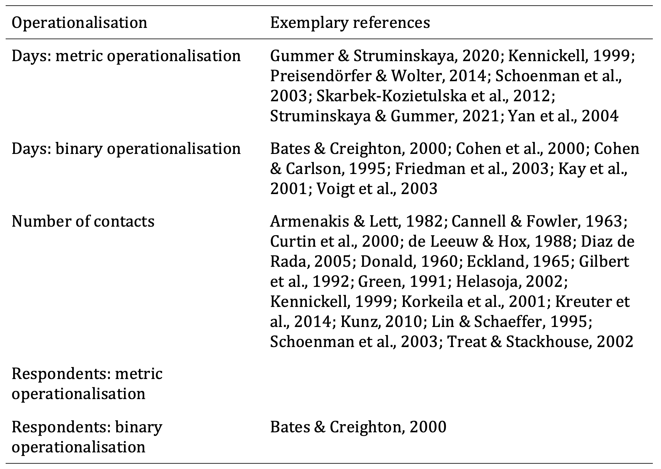
Days: metric operationalisation: Response time can be a metric variable that measures the days until a survey is returned. For this metric operationalisation, each day of delay is an increase in the measurement of response time (e.g., Gummer & Struminskaya, 2020; Kennickell, 1999; Preisendörfer & Wolter, 2014; Skarbek-Kozietulska et al., 2012; Struminskaya & Gummer, 2021). One advantage of this operationalisation is that it offers a richer potential for analysis than does a binary or categorical operationalisation, and it additionally enables a detailed description of respondents’ behaviour. However, one disadvantage of this operationalisation is that it does not come with a built-in threshold for distinguishing “late respondents” from those who participated earlier. This lack of a threshold contrasts with binary or categorial operationalisations, which per se go hand in hand with grouping respondents. Based on the theoretical assumptions presented above as well as the extant research both on this operationalisation and on other data-quality indicators, we expected that longer response time would be related to a higher probability of attrition.
Days: binary operationalisation: It is relatively common in research on response time to choose a threshold for separating early and late respondents. In this case, a response before a given day is treated as an early response, and a response after this day is treated as a late response (Friedman et al., 2003). One common threshold is the date on which a reminder is sent (Cohen et al., 2000; Cohen & Carlson, 1995; Kay et al., 2001). A binary operationalisation of response time requires thoughts about when to set a threshold. Example thresholds could be one or two weeks after the field start, or even after the first day. Such an early threshold would separate particularly motivated respondents from other respondents. Therefore, setting a threshold of after the first day would identify respondents who are more motivated and thereby least likely to attrit rather than identifying respondents who have lower motivation than others. One advantage of this operationalisation is that it distinguishes “late respondents” from those who have participated earlier. However, one disadvantage of this operationalisation is that thresholds vary across studies, which means that response time that is operationalised using a threshold is often not comparable. Based on the aforementioned theoretical assumptions as well as the extant research both on this operationalisation and on other data-quality indicators, we expected that the category that is related to longer response time would have a higher attrition rate.
Number of contacts: Response time can be measured using the number of contacts or reminders (e.g., 1 vs. ~3) (Curtin et al., 2000; Gilbert et al., 1992; Green, 1991; Helasoja, 2002; Kennickell, 1999; Kreuter et al., 2014; Kunz, 2010; Lin & Schaeffer, 1995). Usually, returns per day are highest around field start and decrease over time. Additional contacts – such as reminders – typically lead to an increase in returns per day, which is then followed by a decrease. Hence, operationalising response time by using the number of contacts separates respondents who reply after each contact. Advantages of using the number of contacts as the operationalisation of response time include the vast body of available research that has used this operationalisation as well as its design-orientation because contacts are an investment of resources that are used to achieve respondent participation. However, one disadvantage of using the number of contacts as the operationalisation of response time is that we do not know whether respondents who were reminded would have responded without this reminder at a later time. In fact, this operationalisation assumes that this would not be the case. Based on the aforementioned theoretical assumptions we expected that respondents who are contacted more often would be more likely to attrit.
Respondents: metric operationalisation: Response time can be operationalised not only by drawing on the number of days or the number of contacts, but also by taking into account respondents’ return order. For example, it would be possible to measure how many other respondents had returned a survey prior to a given respondent’s return date for the survey. Such a metric operationalisation would analyse respondents’ behaviour relative to the behaviour of other respondents. One advantage of this operationalisation strategy is that it offers the potential to examine respondents who participate early in the field time but later than most other respondents. While these former respondents would be classified as earlier respondents using other operationalisations, they would be classified as later respondents here. As we do not know whether these respondents behave more like early or late respondents, it was important to take this operationalisation into account, which may be especially relevant for surveys with a short field time. One disadvantage of this operationalisation of response time is that not much research has been conducted on it thus far. Based on the aforementioned theoretical assumptions, we expected that respondents who participate later than other respondents would be more likely to attrit.
Respondents: binary operationalisation: It is also possible to distinguish between first or last respondents on the one hand and other respondents on the other hand by using a fixed number, such as the first or last 100 respondents, or a percentage, such as the first or last 10% of respondents, as was done in Bates and Creighton’s (2000) study. From an analytical point of view, the advantage of this operationalisation is that it offers the ability to classify respondents into smaller groups from among all respondents who participated on a given day. Moreover, survey practitioners may want to select a group of a precise size for potential targeted procedures. This operationalisation is the only one that enables researchers to choose the size of the group whose members should be regarded as early or late respondents. However, one disadvantage of using this operationalisation is that a respondent’s response time depends empirically on other respondents’ response time, but this is not actually the case in real life. Drawing on the above-mentioned theoretical background, we expected that respondents who participate among the first group would be less likely to attrit than would later respondents.
Data and methods
In order to investigate the way in which different operationalisations predict attrition, we used data from the GESIS Panel, which is a probability-based mixed-mode (i.e., web and mail) panel survey that collects data every two to three months (Bosnjak et al., 2018). The GESIS Panel was recruited in 2013 and covers respondents who were sampled from the municipal registries of the general population of Germany. Refreshment samples were drawn in 2016, 2018, and 2021.
Before becoming a regular panelist, respondents participated in a face-to-face recruitment interview. The AAPOR Response Rate 1 in the recruitment interview was 35.5% for the first cohort (i.e., the 2013 recruitment) and 33.2% for the second cohort (i.e., the 2016 refreshment). The third and fourth cohorts (i.e., the 2018 and 2021 refreshments, respectively) were not included in the data that we used for the present study. Respondents to the recruitment interview were invited to a self-administered welcome survey. Among all respondents who had agreed to attend the GESIS Panel, 79.9% of the first cohort and 80.5% of the second cohort participated in the welcome survey. Respondents to this survey became regular panelists. Overall, about 65% of respondents participate in the web mode, and mode switches between the waves are not possible.
Every two months, around 5,000 panelists participate in GESIS Panel surveys. Respondents receive a 5-EUR prepaid incentive with every survey invitation, which is sent via postal mail. Web respondents additionally receive an email with a web link to the survey and up to two email reminders – that is, one reminder each both one and two weeks after the field start. The data used in the present study stem from the dataset of the GESIS Panel Extended Edition, Version 35 (GESIS, 2020), which was published in March 2020 and contains 34 waves (2014–2019).
The dependent variable of panel attrition was operationalised as follows: We defined a case as attrition if a respondent had participated in at least one GESIS Panel wave and had ultimately stopped participating before the fourth wave of 2019. Panel attrition can take two forms: First, respondents can actively de-register, and second, respondents who have not responded in three consecutive waves – despite the fact that their invitations were delivered – are not invited to future waves. For each wave, we used a binary indicator of whether a respondent had attritted as a dependent variable for our analyses. If a respondent had stayed in the panel for a particular wave, the variable was coded as 0. If a respondent had attritted after this wave, the variable was coded as 1. If a respondent had already attritted in one of the previous waves, the variable was coded as a missing value. In the following, we introduce the measurements of response time. A table with examples is provided in the appendix.
Days: metric operationalisation: For the metric operationalisation of the response time in days, we calculated the days it took respondents to participate and then send back their surveys in the respective waves. For every respondent and wave, we subtracted the date of the field start from the date of the return of the survey. For web respondents, the return date was measured by the survey software. For mail participants, we took into account the date when the survey agency received the filled-in questionnaire. It should be noted that the same type of postal mail sent from within Germany takes equally long to be delivered within the country, irrespective of the sending or delivery location.
Days: binary operationalisation: For the operationalisation of response time as a response before or after a specific date, we calculated five variables: (i) response on the first day or later, (ii) response after the first online reminder, (iii) response after the second online reminder, (iv) response in the first week or later, and (v) response in the first two weeks or later. Due to the lack of mail respondents who had participated on the first day, we did not estimate the relationship between this operationalisation and panel attrition for these respondents. We also did not estimate the relationship between response after reminders and panel attrition for mail respondents because these respondents had not received reminders. Instead, for both modes, we estimated the effects of participating both in the first week and in the first two weeks. For each operationalisation except for response on the first day, we coded early response as 0 and late response as 1. Response on the first day was coded as 1 if the respondent had participated on the first day and as 0 if they had participated later.
Number of contacts: In order to calculate the number of contacts, we counted the invitation as the first contact, the first reminder as the second contact, and the second reminder as the third contact. Thus, online respondents could have one, two, or three contacts. Mail respondents did not receive any reminders from the GESIS Panel and thus had only one contact. Therefore, we did not estimate the association between the number of contacts and response time for mail respondents. In practice, web respondents had four contacts because they had received the invitation not only via mail, but also via email. We counted the first two contacts as one contact because the two invitations had been received almost simultaneously. Web respondents could not respond to the first mail contact because the link to the questionnaire had not been included in the invitation letter that had been sent via postal mail and had only been available in the email invitation.
Respondents: metric operationalisation: For the operationalisation of response time as the proportion of panel members who had participated prior to a given respondent, we first separated web and mail respondents. Then, we ordered the two subsamples based on how quickly the respondents had returned the survey, and we assigned numbers to the respondents in this order. For web respondents, we could calculate the exact order by relying on the time stamps of their participation. For the mail respondents, we sorted them by relying on the time stamps provided by the postal service provider. For each subsample, we calculated both how many respondents had participated in the respective waves and how many respondents had returned their survey prior to a given respondent.
Respondents: binary operationalisation: For respondents who had responded prior to – or later than – other respondents, we compared five thresholds: 5%, 10%, 50%, 90%, and 95%. We contrasted the respondents who had participated before a certain threshold with the respondents who had participated after this threshold. We chose the first and last 5% and 10% of respondents as well as an equal division of the sample (i.e., 50%) in order to concentrate not only on late respondents, but also on those who had responded early.
In Table 2, the descriptive statistics – that is, the ranges, means, and standard deviations – of the variables used in the analyses are grouped by survey mode. Generally, mail respondents tended to participate later, which may have been the result of the different response processes.
Table 2: Description of the variables used in the analysis
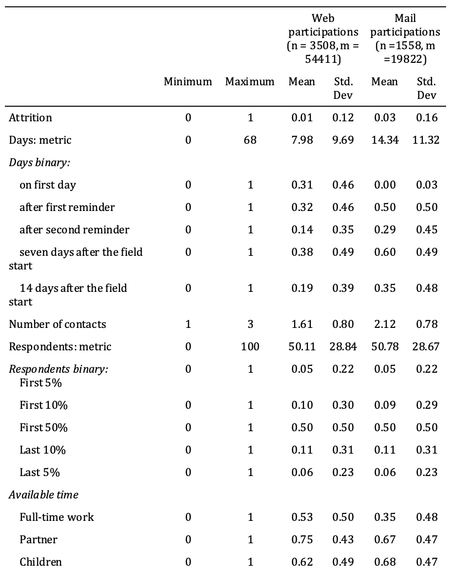
Note: n = number of individuals, m = number of person*wave cases. Among all respondents, 32.22% of web respondents and 43.10% of mail respondents attrited.
We estimated 22 random-effects logistic panel regression models via the maximum likelihood of panel attrition to the following wave, which was 13 models for the web mode and 9 models for the mail mode. The models differed in their operationalisation of response time. As web and mail respondents were treated differently in the surveying process, their response time also differed. For example, mail respondents had to take the survey to a mailbox in order to send it to the researchers, whereas web respondents did not have to take any additional steps beyond answering the questions. This additional step may have delayed the response process for mail respondents but did not affect web participants. All operationalisations of response time were calculated for each wave in which a respondent had participated. Below, we first examine operationalisations of the number of days (Days: metric operationalisation and Days: binary operationalisation) before turning to the number of contacts (Number of contacts) followed by the two operationalisations for other respondents (Respondents: metric operationalisation and Respondents: binary operationalisation).
Our models can be described as
(1) 
where i is the respondent, t is the wave, t+1 is the following wave,  is an intercept,
  represents the regression coefficients,
  is an error term that is different for each individual in every wave, and
  is an error term that includes a set of random variables. A detailed description of the method can be found in Allison (2009).
We analysed the data on all panelists who had participated in at least one GESIS Panel wave and who had not switched from mail to web mode. As a mode switch had been possible during one web-push event in 2018, during which 272 panelists switched modes, we excluded these panelists from our analyses, which left 3,508 web respondents and 1,558 mail respondents. The random-effects method enabled us to compare respondents who had attritted with those who had not. Contrary to fixed-effects models, respondents who had stayed in the panel were included in the random-effects analysis. This decision was important for the comparison of correctly predicted attrition (CPA) and overall correct predictions (OCP), which we used to compare model accuracy. Another example of using this method can be found in Boehmke & Greenwell (2019). In our models, we controlled for previous participation in the panel by including the following control variables: education, factors that influence available time (i.e., working full time, having a partner, and having children), and the evaluation of the previous panel wave (i.e., as difficult, diverse, important, interesting, long, or overly personal). Previous participation was measured as a metric count of the number of survey waves in which the respondent had already participated. Education was considered in three binary variables (i.e., a low, medium, or high level of education) and reflected each respondent’s highest educational degree. Working full time, having a partner, and having children were all considered binary variables, with 0 indicating that the description did not apply to the respondent and 1 indicating that it did apply. Previous survey experience reflected the individual evaluation of the last survey and could range from 1 (i.e., “not at all”) to 5 (i.e., “very”). Available time, survey experience, the number of times a respondent had previously participated, and education could all be argued to be related to both survey response time and panel attrition; therefore, we decided to include these items in order to account for confounding effects.
In order to compare how well the different operationalisations of response time predicted attrition, we assessed the correctness of the model’s prediction of attrition. Each model estimated the predicted probability that each respondent in each wave (respondent*wave case) would attrit from the panel. This estimation enabled us to compare the calculated prediction of attrition with the actual attrition provided by our data – that is, whether or not a respondent had attritted after the respective wave. Thus, this comparison revealed the percentage of all cases of attrition that had been correctly predicted by each model, with the minimum value being 0 and the maximum being 100. When the group size of respondent*wave cases with a high probability of attrition increased, the number of predicted cases of attrition also increased. However, in this case, many panelists who had stayed in a panel were also predicted to attrit, which led to a high number of false predictions regarding respondents who had stayed. Therefore, we added correctly predicted attrition and correctly predicted staying as a method of examining the overall performance of the models. The sum is our second indicator – that is, overall correct predictions. We multiplied both indicators – that is, correctly predicted attrition and overall correct predictions – and ranked the operationalisations based on this product (i.e., correctly predicted to attrite × overall correct predictions).
The first step for calculating correctly predicted attrition was to estimate the probability by which each respondent would attrit. For each operationalisation, we made this calculation based on our regression models. The second step was to compare the probability of attriting with a threshold in order to determine whether respondents were predicted to stay or attrit. As the threshold selection was arbitrary, we randomly drew one individual threshold for every respondent out of the range of 90% of all predictions. The thresholds were distributed uniformly. All respondents with a higher probability of attriting than the threshold were predicted to attrit, and all respondents with a lower probability of attritting than the threshold were predicted to stay in the panel. In order to enable comparability, each respondent’s individual threshold had to remain the same for all the models that were compared. Whenever the aim is to identify most cases of future attrition, the threshold should be chosen empirically by evaluating the correct predictions of attrition and the correct predictions overall.
Results
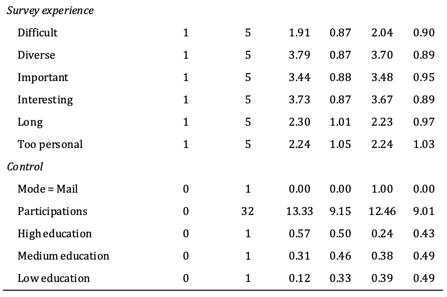
Our results are presented in Table 3. The size of the regression coefficients – which are presented in Column 2 (i.e., “Coefficients”) – is of smaller relevance to us. For most of the operationalisations, we found a statistically significant relationship between response time and panel attrition. It is unexpected that online respondents who participated on the first day, among the first 10% and among the first 50% were more likely to attrit than later respondents. The same can be found for mail participants who participated among the first 50%. This may be reason for a neglectable difference or may show that participation timing has a nonlinear relationship to panel attrition. However, the main results of the analysis pertain to the amount of attrition that each model correctly predicted (i.e., “CPA”, Column 4) and to the percentage of correct predictions (i.e., “OCP”, Column 5) made by each model.
Table 3: Results of random-effects logistic regressions of panel attrition on different operationalisations of response time (34 waves)
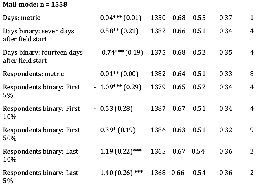
Note: Response on the first day could not be estimated for mail respondents due to a dearth of cases. “Number of contacts” and “after first/second reminder” were omitted for mail participants because these participants had not received reminders. * = p<0.05, ** = p<0.01, *** = p<0.001, standard errors in parentheses. Coefficient = coefficient of a random-effects logistic regression, AIC = Akaike information criterion, CPA = correctly predicted attrition, OCP = overall correct predictions. CPA, OCP, and the product of both all range from 0 to 100, where 0 means no correct predictions and 100 means that all cases were correctly predicted. The “Rank” column shows the ranking among the modes based on the product of the CPA and OCP (the higher, the better).
Our models reveal that a metric operationalisation of response time that used the days until survey return correctly predicted 61% of attrition among web respondents. Among mail respondents, this value was higher. Moreover, the model that included days until survey return as a metric variable correctly predicted 68% of attrition.
An analysis of response on the first day was only relevant for web respondents, and 59% of attrition was correctly predicted using this model. The analyses of response after the first and second reminders were also relevant only for web respondents. 62% of attrition among web respondents was correctly predicted by the model that used response after the first reminder, and 60% of attrition among web participants was correctly predicted by the model that used response after the second reminder. The model that used response after seven days correctly predicted 64% of attrition among web panelists and 66% of attrition among mail-mode panelists. The model that used response after 14 days correctly predicted 59% of attrition among web respondents and 68% of attrition among mail respondents. When the number of contacts was used to predict attrition among web respondents, this model correctly predicted 62% of attrition.
When response time was operationalised as the proportion of panel members who had participated before a given respondent, this model correctly predicted 64% of attrition in both modes. Models that included an operationalisation of response time for whether a respondent had been among the first 5% of respondents to return a survey correctly predicted 60% of attrition for web panelists and 65% of attrition for mail panelists. When response time was operationalised as being among the first 10% of respondents to participate or not, this model correctly predicted 62% of attrition among web respondents and 67% of attrition among mail respondents. The model with an operationalisation of response time that split the first 50% and the last 50% of participation responses correctly predicted 63% of attrition for both web panelists and mail panelists. The models that included the operationalisation of response time as being among the latest 10% to respond correctly predicted 60% of attrition for web panelists and 67% of attrition for mail panelists. When response time was defined based on whether or not a respondent had been among the latest 5% to respond, this model correctly predicted 58% of attrition for web respondents and 66% of attrition for mail respondents.
Overall, the 22 above-described models predicted attrition similarly well, which can also be seen in the close range of the AICs. In order to fairly evaluate these models, the OCP must be taken into account. The overall correct predictions are also similar to one another. There are three possible explanations for this similarity: First, the operationalisation may truly have had a similar relationship to attrition. Second, the similarity could be attributed to the random threshold, which works well when a variable is equally distributed. In our case, we had a skewed distribution, with which the randomly chosen threshold did not fit very well. In cases for which maximising correct predictions is more important than finding a fair method of comparing models, thresholds should be chosen empirically based on the threshold at which the highest OCP can be predicted. Third, the models predicted similar relationships to attrition because the covariates were identical. We believe that all these explanations apply to a certain extent, but the similarity between the correct predictions of attrition can be especially attributed to the third explanation. Two models that share all variables except for one – which was differently operationalised in the two models – should lead to similar predictions of attrition. In order to be able to more easily evaluate the models, Column 6 provides the product of the CPA and OCP. The seventh column (i.e., “Ranking”) provides a ranking of the operationalisations based on the product of the CPA and OCP. As we can see, for web respondents, response time can predict attrition best when it is operationalised either (i) as response before or after seven days after the field start or (ii) as a metric share of prior respondents. For mail respondents, the metric operationalisation of response time works best. Due to the similarity of the results, we recommend that future work that investigates response time conduct a robustness check using multiple operationalisations.
Conclusion & discussion
In the present study, we operationalised response time in multiple ways and estimated the association between each operationalisation and panel attrition. Then, we compared the predictions of attrition that had been estimated by each model. We focused on 13 operationalisations of response time that are commonly used in the literature. The operationalisations were based on (i) the number of days it had taken a respondent to respond, (ii) the number of contacts, and (iii) the proportion of respondents who had participated prior to a given respondent. We found that many – albeit not all – of the operationalisations of response time were significantly related to panel attrition. The regression models predicted attrition similarly well. With regard to the mixed findings in the extant literature, the source of the variance was clearly not the operationalisation of response time, at least not when panel attrition was the variable of interest. Instead, the mixed findings may be attributed to different survey design features, such as field time or response rate.
Almost all of the operationalisations in our study were significantly related to panel attrition, and these operationalisations resembled one another in terms of both how well they could predict attrition and the accuracy of their overall predictions. Although the predictions of attrition were similar, we found that the operationalisations of response time as a metric share of prior respondents and as response before or after seven days after the field start worked best for online respondents and that the operationalisation of response time as a metric count of days until response worked best for mail respondents. Using these operationalisations, the balance between overall correct predictions and correctly predicted attrition was better than when using the alternative operationalisations with the data we used. One drawback of most of the operationalisations of response time that were applied in our study was that a variable that offered metric information – namely the day of the response or the share of prior respondents – was only used as a binary variable. A metric variable would have offered a richer potential for analysis, and the behaviour of the respondents could have been analysed in greater detail. Thus, when researching response time, it may also be advisable to apply a metric operationalisation.
The present study is not without limitations. First, we only focused on the association between the operationalisations of response time and panel attrition. However, other data-quality indicators also exist, such as item nonresponse, straightlining, and the consistency between two measurements, any of which can be associated with response time. Future studies should thus examine the impact of different operationalisations of response time on these data-quality indicators. Second, our study considered the entire process of participation in our operationalisation of response time. In other words, the time it took a response to reach the researchers was counted for the operationalisations of response time in the mail mode. An alternative would have been to count only the time it took a participant to respond. Indeed, after responding, mail-mode participants still had to take the questionnaire to a mailbox. We regard this process as an important part of participation; however, it is possible that this process is not relevant to other studies. Third, the operationalisations of response time could not always be applied to the mail mode and were thus not always disjointed. For instance, reminders were sent on a specific day, and we thus cannot know whether a given response was related to the day or to the reminder. This distinction could be experimentally varied in a future study.
Despite these limitations, our study offers added value for survey practitioners and survey methodologists alike. Indeed, it provides a summary of many operationalisations of response time and also indicates the advantages and disadvantages of the different operationalisations. Our method can aid survey practitioners in identifying potential future attrition, and it can help survey methodologists in determining which operationalisation should be used in future studies on response time. Survey practitioners can easily test which respondents are most likely to attrit by evaluating respondents’ response time. This process is easy to implement and does not require much time or many resources; therefore, the test can be performed after each survey wave. However, survey practitioners should establish guidelines as to how to target interventions (e.g., regarding which respondents to address) that fit their survey with respect to aspects such as field length and attrition rate. In order to establish such rules, practitioners could evaluate questions such as the budget needed for the interventions, the size of the interventions, and the number of respondents who should be targeted by the interventions. Particularly late respondents could be the target of cost-effective interventions, such as additional incentives. Survey methodologists could additionally apply the method used in our study to other time-related data (e.g., website-login timestamps) and compare the way in which different operationalisations of these data are related to a given variable of interest. In terms of response time, our study revealed that the specific operationalisation is of smaller importance when predicting attrition. Hence, of all the operationalisations examined in our study, researchers are free to use the operationalisation that is easiest for them to calculate.
Appendix
In order to illustrate the different operationalisations of response time, in Table A1, we use three fictional respondents and provide exemplary operationalisations of their response time for one wave. This table describes the values for the operationalisations of three fictional respondents, one of whom participated on the first day, by which point in time, 2% of all respondents had already participated. The second respondent participated after three days, by which point in time, 40% of all respondents had already participated. The third respondent participated after 50 days, by which point in time, 98% of all the respondents had already participated.
Table A1: Exemplary response times, and their operationalisations
References
- Allison, P. D. (2009). Fixed effects regression models. SAGE publications.
- Armenakis, A. A., & Lett, W. L. (1982). Sponsorship and follow-up effects on response quality of mail surveys. Journal of Business Research, 10(2), 251– https://doi.org/10.1016/0148-2963(82)90031-5
- Bates, N., & Creighton, K. (2000). The last five percent: What can we learn from difficult interviews? In Proceedings of the Annual Meetings of the American Statistical Association, 13-17.
- Bethlehem, J. G. (2002). Weighting nonresponse adjustments based on auxiliary information. In R. Groves, D. A. Dillman, J. L. Eltinge & R. J. Little (Eds.) Survey Nonresponse. Wiley
- Boehmke, B., & Greenwell, B. (2019). Hands-on machine learning with R. Chapman and Hall/CRC.
- Bollinger, C. R., & David, M. H. (2001). Estimation with response error and nonresponse: Food-stamp participation in the SIPP. Journal of Business & Economic Statistics, 19(2), 129–141. https://doi.org/10.1021/jf0483366
- Bosnjak, M., Dannwolf, T., Enderle, T., Schaurer, I., Struminskaya, B., Tanner, A., & Weyandt, K. W. (2018). Establishing an Open Probability-Based Mixed-Mode Panel of the General Population in Germany: The GESIS Panel. Social Science Computer Review, 36(1), 103– https://doi.org/10.1177/0894439317697949
- Brehm, S. S., & Brehm, J. W. (2013). Psychological reactance: A theory of freedom and control. Academic Press.
- Cannell, C. F., & Fowler, F. J. (1963). Comparison of a self-enumerative procedure and a personal interview: A validity study. Public Opinion Quarterly, 27(2), 250– https://doi.org/10.1086/267165
- Cohen, S. B., & Carlson, B. L. (1995). Characteristics of Reluctant Respondents in the National Medical Expenditure Survey. Journal of Economic and Social Measurement, 21(4), 269– https://doi.org/10.3233/JEM-1995-21402
- Cohen, S. B., Machlin, S. R., & Branscome, J. M. (2000). Patterns of survey attrition and reluctant response in the 1996 medical expenditure panel survey. Health Services and Outcomes Research Methodology, 1(2), 131–148. https://doi.org/10.1023/A:1012543121850
- Curtin, R., Presser, S., & Singer, E. (2000). The Effects of Response Rate Changes on the Index of Consumer Sentiment. Public Opinion Quarterly, 64(4), 413– https://doi.org/10.1086/318638
- de Leeuw, E. D., & Hox, J. J. (1988). Artifacts in Mail Surveys: The Influence of Dillman’s Total Design Method on the Quality of the Responses. In W. E. Saris and I. N. Gallhofer (Eds.) Sociometric Research. 2: Data Analysis. (pp. 61–73). Springer. https://doi.org/10.1007/978-1-349-19054-6_3
- Diaz de Rada, V. (2005). The Effect of Follow-up Mailings on The Response Rate and Response Quality in Mail Surveys. Quality & Quantity, 39(1), 1– https://doi.org/10.1007/s11135-004-5950-5
- Donald, M. N. (1960). Implications of Nonresponse for the Interpretation of Mail Questionnaire Data. Public Opinion Quarterly, 24(1), 99-114. https://doi.org/10.1086/266934
- Eckland, B. K. (1965). Effects of prodding to increase mail-back returns. Journal of Applied Psychology, 49(3), 165– https://doi.org/10.1037/h0021973
- Friedman, E. M., Clusen, N. A., & Hartzell, M. (2003). Better Late? Characteristics of Late Respondents to a Health Care Survey. Proceedings of the Survey Research Methods Section of the American Statistical Association, 992–98.
- (2020). GESIS Panel—Extended Edition. GESIS, Cologne. ZA5664 Datafile Version 35.0.0. https://doi.org/10.4232/1.13435
- Gilbert, G. H., Longmate, J., & Branch, L. G. (1992). Factors influencing the effectiveness of mailed health surveys. Public Health Reports, 107(5), 576-584.
- Green, K. E. (1991). Reluctant Respondents: Differences between Early, Late, and Nonresponders to a Mail Survey. The Journal of Experimental Education, 59(3), 268–276. https://doi.org/10.1080/1991.10806 566
- Groves, R. M. (2005). Survey errors and survey costs. John Wiley & Sons.
- Groves, R. M. (2006). Nonresponse rates and nonresponse bias in household surveys. Public opinion quarterly, 70(5), 646–675.
- Gummer, T., & Struminskaya, B. (2020). Early and Late Participation during the Field Period: Response Timing in a Mixed-Mode Probability-Based Panel Survey. Sociological Methods & Research 0(0), 1-24. https://doi.org/10.1177/0049124120914921
- Helasoja, V. (2002). Late response and item nonresponse in the Finbalt Health Monitor Survey. The European Journal of Public Health, 12(2), 117– https://doi.org/10.1093/eurpub/12.2.117
- Kay, W. R., Boggess, S., Selvavel, K., McMahon, M. F., & Kay, W. R. (2001). The Use of Targeted Incentives to Reluctant Respondents on Response Rate and Data Quality. In Proceedings of the Annual Meeting of the American Statistical Association, 1-7.
- Kennickell, A. B. (2017). What do the ‘late’ cases tell us? Evidence from the 1998 Survey of Consumer Finances. Statistical Journal of the IAO 33(1), 81-92. https://doi.org/10.3233/SJI-160302
- Korkeila, K., Suominen, S., Ahvenainen, J., Ojanlatva, A., Rautava, P., Helenius, H., & Koskenvuo, M. (2001). Non-response and related factors in a nation-wide health survey. European journal of epidemiology, 17(11), 991–999. https://doi.org/10.1023/A:1020016922473
- Kreuter, F. (2013). Improving surveys with paradata: Analytic uses of process information. John Wiley & Sons.
- Kreuter, F., Müller, G., & Trappmann, M. (2014). A Note on Mechanisms Leading to Lower Data Quality of Late or Reluctant Respondents. Sociological Methods & Research, 43(3), 452– https://doi.org/10.1177/0049124113508094
- Kunz, F. (2010). Empirical Findings on the Effects on the Response Rate, the Responses and the Sample Composition. methods, data, analyses, 4(2), 127-155. https://doi.org/10.12758/mda.2010.009.
- Lin, I.-F., & Schaeffer, N. C. (1995). Using survey participants to estimate the impact of nonparticipation. Public Opinion Quarterly, 59(2), 236–258. https://doi.org/10.1086/269471
- Lynn, P., & Lugtig, P. J. (2017). Total Survey Error for Longitudinal Surveys. In P. P. Biemer, E. de Leeuw, S. Eckman, B. Edwards, F. Kreuter, L. E. Lyberg, N. C. Tucker, & B. T. West (), Total Survey Error in Practice (pp. 279–298). John Wiley & Sons, Inc. https://doi.org/10.1002/9781119041702.ch13
- Olson, K. (2013). Do non-response follow-ups improve or reduce data quality? A review of the existing literature. Journal of the Royal Statistical Society: Series A (Statistics in Society), 176(1), 129– https://doi.org/10.1111/j.1467-985X.2012.01042.x
- Preisendörfer, P., & Wolter, F. (2014). Who Is Telling the Truth? A Validation Study on Determinants of Response Behavior in Surveys. Public Opinion Quarterly, 78(1), 126– https://doi.org/10.1093/poq/nft079
- Roßmann, J., & Gummer, T. (2016). Using Paradata to Predict and Correct for Panel Attrition. Social Science Computer Review, 34(3), 312– https://doi.org/10.1177/0894439315587258
- Schoenman, J. A., Berk, M. L., Feldman, J. J., & Singer, A. (2003). Impact Of Differential Response Rates On The Quality Of Data Collected In The CTS Physician Survey. Evaluation & the Health Professions, 26(1), 23– https://doi.org/10.1177/0163278702250077
- Skarbek-Kozietulska, A., Preisendörfer, P., & Wolter, F. (2012). Leugnen oder gestehen? Bestimmungsfaktoren wahrer Antworten in Befragungen. Zeitschrift für Soziologie, 41(1), 5-23. https://doi.org/10.1515/zfsoz-2012-0103
- Struminskaya, B., & Gummer, T. (2022). Risk of Nonresponse Bias and the Length of the Field Period in a Mixed-Mode General Population Panel. Journal of Survey Statistics and Methodology 10(1), 161-182. https://doi.org/10.1093/jssam/smab011
- Treat, J. B., & Stackhouse, H. F. (2002). Demographic comparison between self-response and personal visit interview in Census 2000. Population Research and Policy Review, 21(1), 39–51. https://doi.org/10.1023/A:1016541328818
- Voigt, L. F., Koepsell, T. D., & Daling, J. R. (2003). Characteristics of telephone survey respondents according to willingness to participate. American journal of epidemiology, 157(1), 66–73. https://doi.org/10.1093/aje/kwf185
- Yan, T., Tourangeau, R., & Arens, Z. (2004). When less is more: Are reluctant respondents poor reporters?. In Proceedings of the Annual Meetings of the American Statistical Association. 4632-4651.