


1. Introduction
A turbulent boundary layer over a streamwise change in wall roughness can be considered to be a distillation of flows commonly observed in nature and industry, examples of which include a surface layer where a forest terrain changes to a prairie, and a turbulent boundary layer developing on a ship's hull with patchy biofouling. Understanding the behaviour of the flow downstream of a step-change in roughness and the ability to model the flow evolution are beneficial to atmospheric forecasting, as well as drag estimation for better fuel efficiency.
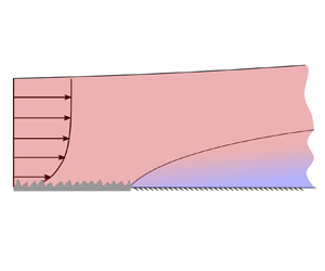
A schematic of the flow configuration is shown in figure 1. A turbulent boundary layer develops on a wall, the roughness of which abruptly changes at  $x=x_0$. Here,
  $x$ represents the streamwise direction and
  $z$ represents the wall-normal direction. The fetch on the downstream surface is then denoted as
  $\hat {x} = x-x_0$. The flow adapts to the new wall condition firstly close to the wall, and the affected region (light blue shaded region) widens farther downstream. This region, where the flow is modified by the new wall condition, is usually referred to as the internal layer or internal boundary layer (IBL), and its thickness is denoted by
  $\delta _i$. The topic has been reviewed by Garratt (Reference Garratt1990), and the application in meteorology has recently been reviewed by Bou-Zeid et al. (Reference Bou-Zeid, Anderson, Katul and Mahrt2020). The flow structures with characteristics of the upstream roughness are considered to persist above the IBL. An equilibrium layer (EL) can also be defined as the near-wall region where the flow has fully adapted to the new surface condition, and its thickness is denoted by
  $\delta _e$. Traditionally,
  $\delta _e$ has been assessed by comparing the mean streamwise velocity profile or shear stress profile scaled by the local friction velocity with the corresponding profile of the downstream surface (Rao, Wyngaard & Coté Reference Rao, Wyngaard and Coté1974). In this study, we define both IBL and EL using the mean velocity profile.

Figure 1. Schematic of a turbulent boundary layer over a step change in surface roughness condition. The roughness transition occurs at  $x_0$, and
  $\hat {x} = x-x_0$ denotes the fetch downstream of the transition.
Predicting the evolution of the flow downstream of a roughness step change, given the surface and upstream flow conditions, has attracted great interest in the past few decades. It has important applications in the site selection of a meteorology measurement tower, where it is desirable to choose a location at a sufficient distance away from the change in surface condition to avoid the ‘leading-edge effects’. The tower should also be submerged in the EL in order to sample the quantities associated with the local wall condition rather than the remnant of upstream structures. A detailed summary of various modelling attempts can be found in the work by Savelyev & Taylor (Reference Savelyev and Taylor2005). A crude rule of thumb to estimate the IBL thickness is  $\delta _i/\hat {x}\approx 1/10$ and
  $\delta _e/\hat {x}\approx 1/200$ (Rao et al. Reference Rao, Wyngaard and Coté1974). Power-law relationships with a form of
  $\delta _i\propto \hat {x}^{\alpha }$ are obtained by empirically fitting to experimentally or numerically generated data, and the exponent varies from 0.2 to 1 across studies (Rouhi, Chung & Hutchins Reference Rouhi, Chung and Hutchins2019). Although these relationships are easy to implement, they are usually obtained from a particular set of surface and flow conditions and cannot be generalised to others.
There are considerable attempts in the literature to theoretically model the flow response to a step change in the wall condition, and they can be classified into two major categories based on the assumptions made. Most of these models are developed in the context of atmospheric surface layers where the canonical mean velocity profile can be approximated by a log-law. The first category of theoretical models is established on the diffusion analogy, which was introduced by Miyake (Reference Miyake1965). In this approach, the IBL is assumed to propagate in the same manner as a passive contaminant, and the growth rate of  $\delta _i$ is proportional to
  $w_{rms}(\delta _i) = (\overline {w^2})^{1/2}$, the vertical diffusion intensity at the interface. That is,
 \begin{equation} \frac{\mathrm{d}\delta_i}{\mathrm{d}t} = A w_{rms}, \end{equation}
where  $A$ is a constant and
  ${\rm d}(\,{\cdot }\,)/{\rm d}(\,{\cdot}\,)$ denotes the total derivative. Using the chain rule, the left-hand side of the equation can be rewritten as
  $\mathrm {d}\delta _i/\mathrm {d}t =(\partial \delta _i/\partial x)({\mathrm{d}\kern0.7pt x}/\mathrm {d}t)$ for a steady state (
 $\partial \delta _i/\partial t = 0$). Assuming
  $\mathrm{d}\kern0.7pt x/\mathrm {d}t = U(\delta _i)$, which is the mean velocity at the interface, the equation above can be rewritten as
 \begin{equation} U(\delta_i)\frac{\mathrm{d}\delta_i}{\mathrm{d}\kern0.7pt x} = A w_{rms}. \end{equation}
After relating the  $w_{rms}$ term to the friction velocity (upstream or downstream) through an assumed proportionality in neutrally stratified flow,
  $w_{rms} = C U_{\tau }$ (
 $C$ is also a constant), determining the velocity at the interface
  $U(\delta _i)$ from a logarithmic profile and prescribing an initial condition of
  $\delta _i|_{\hat {x} = 0}$, (1.2) can be integrated to obtain the final expression of the IBL growth. Models with various expressions of the
  $w_{rms}$ and
  $U(\delta _i)$ terms were developed (Jackson Reference Jackson1976; Panofsky & Dutton Reference Panofsky and Dutton1984; Savelyev & Taylor Reference Savelyev and Taylor2001; Bou-Zeid, Meneveau & Parlange Reference Bou-Zeid, Meneveau and Parlange2004; Yang Reference Yang2016), and it was also extended to non-neutral stability conditions (Savelyev & Taylor Reference Savelyev and Taylor2005).
A second group of models assume a form of the recovering mean velocity profile, and then relate the local wall-shear stress to the growth of the IBL through the streamwise momentum equation. This approach was established in the seminal study of Elliott (Reference Elliott1958), where a piecewise logarithmic velocity profile with a change in slope across the edge of the IBL was used. Shear stress, as derived from the slope of the log-law profile through a ‘mixing-length’ relation, takes the form of a step function, and attempts were made to eliminate the discontinuity at the edge of the IBL by using a velocity profile integrated from a shear-stress profile that linearly changes from the downstream value to the upstream one across the IBL (Panofsky & Townsend Reference Panofsky and Townsend1964). So far in both mean velocity profile models described, the flow above the IBL remains unmodified from that upstream of the step change and no streamwise development of the flow in this region is considered. That is to say, if we denote the upstream velocity profile as  $U_1(z)$ (where
  $z$ is the wall-normal position), then
  $U(z)=U_1(z)$ will hold for all
  $z>\delta _i$. Another way of modelling the flow is to assume that the mean velocity remains constant along a streamline above the IBL, while within the IBL the acceleration of the mean velocity along the same streamline is self-similar (Townsend Reference Townsend1965a,Reference Townsendb, Reference Townsend1966). The mean velocity profiles constructed by Elliott (Reference Elliott1958) and Panofsky & Townsend (Reference Panofsky and Townsend1964) can be incorporated into the Townsend self-similar framework with streamline displacement.
More recently, it has been recognised that the flow in the IBL has not fully adapted to the local wall condition, questioning the applicability of an equilibrium log-law profile, as well as the corresponding mixing-length relation (Antonia & Luxton Reference Antonia and Luxton1972; Shir Reference Shir1972; Rao et al. Reference Rao, Wyngaard and Coté1974; Ismail, Zaki & Durbin Reference Ismail, Zaki and Durbin2018; Rouhi et al. Reference Rouhi, Chung and Hutchins2019). Chamorro & Porté-Agel (Reference Chamorro and Porté-Agel2009) proposed a semiempirical blending model of the recovering mean velocity profile without further incorporating the streamwise evolution. They considered that after a rough-to-smooth transition, the mean velocity profile asymptotes to the new smooth-wall log law at the wall and the upstream rough-wall log law at the edge of the IBL. These two limiting cases are then blended by a log-linear weight function, representing the gradual transition from the local smooth-wall log law to the upstream rough-wall counterpart as  $z/\delta _i$ increases. This model of the velocity profile does not assume a constant or linear distribution of the shear stress in the IBL (as did Elliott (Reference Elliott1958) and Panofsky & Townsend (Reference Panofsky and Townsend1964)). The agreement with measurements in the near-wall region is further improved by prescribing a finite thickness of the EL (Abkar & Porté-Agel Reference Abkar and Porté-Agel2012; Ghaisas Reference Ghaisas2020), or using a log-normal blending function that gives more weight to the smooth-wall profile close to the wall (Li et al. Reference Li, de Silva, Chung, Pullin, Marusic and Hutchins2021).
In addition to the two major categories as discussed above, there have also been other attempts in modelling the flow response to a roughness change. Wood (Reference Wood1982) developed a simple correlation for the IBL thickness from dimensional analysis. Peterson (Reference Peterson1969) adopted a closure of the turbulent shear stress and solved the continuity, momentum and turbulent-energy equations numerically. Van Buren et al. (Reference Van Buren, Floryan, Ding, Hellström and Smits2020) performed a perturbation analysis on the mean-momentum equation and Reynolds stress transport equation of a rough-to-smooth change in a pipe flow, and successfully captured the second-order response in the experimental data.
To summarise, Elliott's original model was formulated for an atmospheric surface layer with no consideration of the gradual adjustment of the flow in the IBL to the new wall condition. In this study, we incorporate modifications that make Elliott's approach valid for a turbulent boundary layer with finite thickness. The inherent difference between the current model and Elliott's original formulation is that we consider a finite thickness of the total boundary layer, and introduce an additional momentum equation to describe its spatial growth. The new model is useful for a wide range of engineering applications where a finite-thickness boundary layer is concerned, such as the flow over patches of biofouling roughness on a ship's hull. A series of refinements will be discussed, including reassessing the assumptions originally made concerning a deep surface layer where  $\delta _i/\delta _{99}$ is small, as well as incorporating the blending velocity profile as detailed in Li et al. (Reference Li, de Silva, Chung, Pullin, Marusic and Hutchins2021).
The streamwise, spanwise and wall-normal directions are represented by  $x$,
$x$,  $y$ and
  $z$. The corresponding time-averaged and fluctuation velocity components are denoted by
  $U$,
$U$,  $V$,
$V$,  $W$ and
  $u$,
$u$,  $v$,
$v$,  $w$, respectively. Quantities upstream and downstream of the rough-to-smooth transition are distinguished by a subscript
  $(\,{\cdot}\,)_1$ and
  $(\,{\cdot }\,)_2$, respectively, and the subscript
  $(\,{\cdot }\,)_0$ represents quantities at the roughness transition (
 $x = x_0$ or just prior to it if there is a jump of that quantity across the roughness transition, see figure 1).
This paper is structured as follows. First, Elliott's original model is summarised in § 2, and its numerical implementation is presented in § 3. The model is then evaluated utilising an experimental dataset covering a wide range of flow parameters (Li et al. Reference Li, de Silva, Chung, Pullin, Marusic and Hutchins2021) in § 3.1. Refinements including considering a wake profile, the streamwise growth of the entire boundary layer, a  $z$-dependent shear stress profile, and the blending velocity profile in the IBL (as discussed in Li et al. (Reference Li, de Silva, Chung, Pullin, Marusic and Hutchins2021)), are added and compared with the original model in § 4. The performance of the new model is assessed in § 5.
2. A brief review of Elliott's model
In the seminal study of Elliott (Reference Elliott1958), a theoretical model predicting the flow recovery from a step change in the surface roughness was established. The flow condition is illustrated in figure 2(a). The incoming flow can be fully described by the roughness length  $z_{01}$ and friction velocity
  $U_{\tau 1}$ of the upstream surface, while the only information about the downstream surface is the roughness length
  $z_{02}$. Both upstream and downstream surfaces are assumed to be in the fully rough regime, and the roughness length can be related to the equivalent sand grain roughness
  $k_s$ by
 \begin{equation} z_0 = k_s\exp(-\kappa A'_{fr}), \end{equation}
where  $A'_{fr}=8.5$ is the fully rough intercept for sand grain roughness (Nikuradse Reference Nikuradse1950). An extension of the model is to consider that either the upstream or downstream surface is fully smooth, and the roughness length will then be related to the viscous wall unit through
 \begin{equation} z_0 = \frac{\nu}{U_{\tau }}\exp(-\kappa B), \end{equation}
where  $B$ is the smooth-wall intercept,
  $U_{\tau }$ is the local friction velocity and
  $\nu$ is the kinematic viscosity of air. Here, the constant values are chosen as
  $\kappa = 0.384$,
  $B = 4.17$ (Chauhan, Monkewitz & Nagib Reference Chauhan, Monkewitz and Nagib2009). In the scenario of a rough-to-smooth transition, the downstream roughness length
  $z_{02}$ is directly related to the local friction velocity, which can vary significantly with
  $\hat {x}$, particularly for
  $\hat {x}/\delta _0 \lesssim 2$ (Li et al. Reference Li, de Silva, Chung, Pullin, Marusic and Hutchins2021).

Figure 2. (a) Sketch of the flow over a roughness change in the streamwise direction. The IBL is shown by blue, and the outer layer is shown by red. The control volume used to obtain (2.5) is bounded by the dashed line. (b) Sketch of the mean velocity profile in Elliott's model corresponding to the flow condition in (a). The local inner log-law profile is shown by blue, and the outer log-law profile is shown by red, and a rough-to-smooth transition ( $z_{01}>z_{02}$) is assumed in the plot.
After the roughness transition at  $x = x_0$ (i.e.
  $\hat {x} = 0$), an IBL containing the modified flow develops on the downstream surface and a local friction velocity
  $U_{\tau 2}$ evolves with the growth of the IBL. In this system, the roughness lengths
  $z_{01}$ and
  $z_{02}$ are known. Here,
  $U_{\tau 1}$ is also given and assumed to be constant, therefore, we have
  $U_{\tau 1}(\hat {x}) = U_{\tau 1}(0) \equiv U_{\tau 0}$, to be consistent with previous notations. This leaves two unknowns,
  $\delta _i(\hat {x})$ and
  $U_{\tau 2}(\hat {x})$, as functions of
  $\hat {x}$, the fetch on the downstream surface. Therefore, two equations are required to close the system and provide solutions of
  $\delta _i$ and
  $U_{\tau 2}$.
Elliott approximated the recovering mean velocity profile with a piecewise logarithmic function (illustrated in figure 2b),
 \begin{equation} U(z) = \begin{cases}
\dfrac{U_{\tau 1}}{\kappa} \ln(z/z_{01}), &
z\geqslant\delta_i\\ \dfrac{U_{\tau 2}}{\kappa}
\ln(z/z_{02}), & z<\delta_i,\\
\end{cases}\end{equation}
\begin{equation} U(z) = \begin{cases}
\dfrac{U_{\tau 1}}{\kappa} \ln(z/z_{01}), &
z\geqslant\delta_i\\ \dfrac{U_{\tau 2}}{\kappa}
\ln(z/z_{02}), & z<\delta_i,\\
\end{cases}\end{equation}
which implicitly assumes that the mean velocity profile within the IBL immediately adapts to the local wall condition (i.e. that  $\delta _i = \delta _e$). From this expression of the mean velocity profile, the first equation to close the system rises naturally as the matching condition, i.e. the two log laws intersecting at
  $z = \delta _i$:
 \begin{equation} \frac{U_{\tau 1}}{\kappa} \ln(\delta_i/z_{01}) = \frac{U_{\tau 2}}{\kappa} \ln(\delta_i/z_{02}). \end{equation}
A series of the velocity profiles with various  $\delta _i$ values are shown in figure 3.

Figure 3. An illustration of the mean velocity profile (2.3) for (a)  $z_{01}>z_{02}$ (rough-to-smooth) and (b)
  $z_{01}< z_{02}$ (smooth-to-rough). The red lines in both panels are the upstream velocity profile, and the blue line is the velocity profile within the IBL at
  $\hat {x} = 0$. The black dots are a few representative locations of
  $\delta _i$ farther downstream and the black dashed lines are the velocity profile within the IBL corresponding to these
  $\delta _i$ values.
Considering a control volume which has a streamwise width of  ${\rm d}\kern0.7pt x$ and is bounded by the wall and the IBL height (shown by the dashed line in figure 2a), and balancing the streamwise momentum fluxes across the control surface with the net shear stress applied on the top and bottom surfaces, a second equation can be obtained,
 \begin{equation} \frac{\mathrm{d}}{\mathrm{d}\kern0.7pt x}\int_{z_{02}}^{\delta_i}U^2(\hat{x},z)\,\mathrm{d}z-U_i(\hat{x}) \frac{\mathrm{d}}{\mathrm{d}\kern0.7pt x}\int_{z_{02}}^{\delta_i}U(\hat{x},z)\,\mathrm{d}z = \frac{\Delta \tau(\hat{x})}{\rho}, \end{equation}
where  $\Delta \tau (\hat {x}) = \tau (\hat {x},\delta _i(\hat {x}))-\tau (\hat {x},0)$. The shear stress at the wall is
  $\tau (\hat {x},0) = \rho U^2_{\tau 2}(\hat {x})$ by definition, while Elliott assumed that the upper boundary of the control volume resides within the constant-stress layer which preserves the shear stress of the upstream surface, i.e.
  $\tau (\hat {x},\delta _i) = \rho U^2_{\tau 1}$. Therefore, the net shear stress term can be expressed as
  $\Delta \tau (\hat {x}) = \rho U_{\tau 1}^2- \rho U_{\tau 2}^2(\hat {x})$. The lower bound of the integral,
  $z_{02}$, is chosen as the lowest wall-normal position where the logarithmic
  $U$ profile is negative according to the mean velocity profile in (2.3). To simplify the notation, we denote the mean velocity at
  $z = \delta _i$ as
  $U_i$, i.e.
  $U_i(\hat {x})\equiv U(\hat {x},\delta _i)$.
With these two equations (2.4) and (2.5), the system will be closed and the evolution of  $U_{\tau 2}$ and
  $\delta _i$ can be solved. The growth of
  $\delta _i$ is driven by the source term,
  $\Delta \tau (\hat {x})/\rho$, which is essentially the difference in the shear stress between the lower and upper control surfaces. The recovering downstream friction velocity
  $U_{\tau 2}(\hat {x})$ asymptotes to
  $U_{\tau 1}$. In fact, the streamwise evolution of the flow will only terminate when
  $U_{\tau 2}=U_{\tau 1}$, which is expected at an infinitely long fetch where
  $\delta _i\gg \max (z_{01},z_{02})$. That is to say, when
  $\delta _i$ is infinitely large, in figure 2(b) the velocity profile in the IBL (blue line) will eventually be parallel with the upstream velocity profile (red line), thus
  $U_{\tau 2} = U_{\tau 1}$.
3. Numerical implementation of Elliott's 1958 model
Elliott (Reference Elliott1958) solved the ordinary differential equation (ODE) (2.5) analytically. This approach is highly dependent on the analytical form of the mean velocity profile and it can be tedious or even impossible to find an algebraic solution when the functional form of the mean velocity profile changes. Alternatively, we may consider the integral form of (2.5). We first consider a change of variable with  $\delta _i$ replacing
  $\hat {x}$ as the independent variable, and apply substitutions
 \begin{equation} G_1(\delta_i) = \int_{z_{02}}^{\delta_i}U(\delta_i,z)\,\mathrm{d}z,\quad G_2(\delta_i) = \int_{z_{02}}^{\delta_i}U^2(\delta_i,z)\,\mathrm{d}z \end{equation}
to (2.5), resulting in
 \begin{equation} \frac{\mathrm{d}G_2\left(\delta_i\right)}{\mathrm{d}\kern0.7pt x\left(\delta_i\right)}-U_i\left(\delta_i\right) \frac{\mathrm{d}G_1\left(\delta_i\right)}{\mathrm{d}\kern0.7pt x\left(\delta_i\right)} = \frac{\Delta \tau\left(\delta_i\right)}{\rho} . \end{equation}
Multiplying both sides of the equation by  $\mathrm{d}\kern0.7pt x(\delta _i)$ and integrating with respect to
  $G_1$ and
  $G_2$ on the left-hand side, and
  $x$ on the right-hand side gives
 \begin{equation} \hat{x}(\delta_i) = \int_{G_2(\delta_i(0))}^{G_2(\delta_i)} \frac{\rho}{\Delta \tau(\delta_i)}\mathrm{d}G_2(\delta_i)-\int_{G_1(\delta_i(0))}^{G_1(\delta_i)} \frac{\rho U_i(\delta_i)}{\Delta \tau(\delta_i)}\mathrm{d}G_1(\delta_i) , \end{equation}
which is equivalent to (2.5) when  $\Delta \tau$ is non-zero.
Here in the integral form (3.3),  $\delta _i$ rather than
  $\hat {x}$ is considered as the independent variable for computational convenience, provided that
  $\mathrm {d} \delta _i/\mathrm {d}\hat {x}\neq 0$. Thus,
  $U_i$ will be a function of
  $\delta _i$ and the two-dimensional mean velocity field
  $U(\hat {x},z)$ will be a function of
  $\delta _i$ and
  $z$ instead. The initial condition of the IBL evolution is
  $\delta _{i}(0)$, i.e.
  $\delta _i(0) = \delta _i$ at
  $\hat {x} = 0$. The choice of
  $\delta _i(0)$, provided small, will only lead to a constant displacement in
  $\hat {x}$ without changing the shape of the predicted
  $\delta _i$ trajectories (see Appendix C). In practice, an array of
  $\delta _i$ locations is first generated, which subsequently determines
  $U_{\tau 2}(\delta _i)$ and the mean velocity profile
  $U(\delta _i,z)$ using (2.4), the relation from matching the mean velocity profile at
  $\delta _i$. The fetch
  $\hat {x}$ corresponding to each
  $\delta _i$ will then be computed from (3.3) numerically. Compared with the original solution of Elliott (Reference Elliott1958), this approach can easily accommodate velocity profiles with more complicated functional forms, which will largely serve our intention in refining the model assumptions. We also note that when presenting the model predictions graphically, we revert to the previous convention of plotting physical quantities against
  $\hat {x}$ to be consistent with the literature. From here on, this model will be referred to as the E58 model.
3.1. Evaluating the E58 model
We first evaluate the E58 model by comparing the experimental data (Li et al. Reference Li, de Silva, Chung, Pullin, Marusic and Hutchins2021) with predictions at matched flow conditions. Two groups of wind tunnel experiments are designed to separately examine the effect of friction Reynolds number and roughness Reynolds number on the flow recovery from a rough-to-smooth change. The friction and roughness Reynolds numbers are defined as  $Re_{\tau 0}\equiv U_{\tau 0}\delta _0/\nu$ and
  $k_{s0}^+\equiv U_{\tau 0}k_s/\nu$, respectively, and are both evaluated based on conditions over the rough surface just upstream of the roughness transition. The Group-Re consists of measurements with varying
  $Re_{\tau 0}$ while holding
  $k_{s0}^+$ constant, while Group-ks measurements vary
  $k_{s0}^+$ while holding
  $Re_{\tau 0}$ constant. The same P24 grit sandpaper is used in all cases, ensuring a constant
  $k_s$, and the variation in
  $Re_{\tau 0}$ and
  $k_{s0}^+$ is achieved by adjusting
  $U_{\infty }$, the free stream velocity, and
  $x_0$, the streamwise length of the sandpaper patch. The magnitude of the surface roughness change is denoted by
  $M\equiv \ln (z_{02}/z_{01})$, where
  $z_{02}$ is calculated from the maximum
  $U_{\tau 2}$ measured downstream of the transition. Legends and flow conditions of the cases are summarised in table 1 and the
  $Re_{\tau 0}$–
 $k_{s0}^+$ parameter space is shown in figure 4. For further experimental details of these cases, readers are referred to the paper by Li et al. (Reference Li, de Silva, Chung, Pullin, Marusic and Hutchins2021).

Figure 4. Flow conditions ( $Re_{\tau 0}$ and
  $k_{s0}^+$) at the immediate upstream of the roughness transition of all cases. All symbols are defined in table 1. The horizontal line is at
  $k_{s0}^+ = 160$, and the vertical line is at
  $Re_{\tau 0} = 14\,500$. The two dashed lines show the cases with matched
  $\delta _{0}/k_s$ of 64 and 133. Adapted from Li et al. (Reference Li, de Silva, Chung, Pullin, Marusic and Hutchins2021).
Table 1. Summary of the experimental cases. The friction velocity  $U_{\tau 0}$ employed in calculating
  $Re_{\tau 0}$ and
  $k^+_{s0}$ is obtained over the rough fetch just upstream of the rough-to-smooth transition. Note that case Re14ks16 is shared between Group-Re and Group-ks, therefore its symbol can take either pink or blue colour in the corresponding group. Adapted from Li et al. (Reference Li, de Silva, Chung, Pullin, Marusic and Hutchins2021).

In the original formulation of Elliott's model, the incoming flow is a deep surface layer where neither  $\delta _0$ nor
  $U_{\infty }$ (therefore
  $C_f$) is defined. It is also applicable to a flat plate boundary layer with a finite thickness where
  $\delta _i$ is only a small fraction of the entire boundary layer. Based on the dimensional argument, the flow should be independent of
  $\delta _0$ in the limit of small
  $\delta _i/\delta _0$. For a smooth downstream surface, the piecewise mean velocity profile (2.3) can be rewritten as
 \begin{equation} U(z) = \begin{cases}
\dfrac{U_{\tau 1}}{\kappa} \ln(z/z_{01}), &
z\geqslant\delta_i\\ U_{\tau 2}\left(\dfrac{1}{\kappa}
\ln(zU_{\tau 2}/\nu)+B\right), & z<\delta_i,
\end{cases}\end{equation}
\begin{equation} U(z) = \begin{cases}
\dfrac{U_{\tau 1}}{\kappa} \ln(z/z_{01}), &
z\geqslant\delta_i\\ U_{\tau 2}\left(\dfrac{1}{\kappa}
\ln(zU_{\tau 2}/\nu)+B\right), & z<\delta_i,
\end{cases}\end{equation}
and the kinematic viscosity of the fluid  $\nu$ instead of a roughness length
  $z_{02}$ is introduced to the problem. When choosing
  $U_{\tau 0}$ as the velocity scale and
  $\nu /U_{\tau 0}$ as the length scale, the incoming flow condition can be fully described by a non-dimensional number
  $k_{s0}^+$, provided that
  $\delta _0$ is large so it does not enter the problem. This implies that for the E58 model, both
  $U_{\tau 2}/U_{\tau 0}$ and
  $\delta _i U_{\tau 0}/\nu$ in Group-Re, where
  $k_{s0}^+$ is held constant, should collapse to a single trend despite the changes in
  $Re_{\tau 0}$. The comparison of these theoretical results with experimental data is discussed below.
3.2. Friction velocity  $U_{\tau 2}$

The measured and predicted recovering friction velocity  $U_{\tau 2}$ on the downstream surface is plotted against fetch
  $\hat {x}$ in figure 5, using
  $U_{\tau 0}$ and
  $\nu /U_{\tau 0}$ as the velocity and length scales, respectively. The Group-Re results are shown in figure 5(a), where a single curve represents the prediction of the E58 model for all four cases, since
  $Re_{\tau 0}$ (essentially the outer length scale) was not a parameter in the original model. Over a limited range of
  $\hat {x}U_{\tau 0}/\nu <1\times 10^5$, the measurements follow the prediction closely with no distinguishable trend with
  $Re_{\tau 0}$. The Group-ks data are presented in figure 5(b), where a greater drop in the friction velocity downstream is observed with a higher
  $k_{s0}^+$. The good agreement between the data points and the model prediction indicates that such a dependence on
  $k_{s0}^+$ is generally well captured by the E58 model.

Figure 5. Friction velocities on the smooth surface normalised by  $U_{\tau 0}$, the friction velocity on the rough surface versus the viscous-scaled fetch
  $\hat {x} U_{\tau 0}/\nu$ for (a) Group-Re and (b) Group-ks. Panels (c) and (d) are the corresponding magnified view in the near field. The solid lines in all figures are predictions using the E58 model with
  $k_{s0}^+ = 160$, while the dashed and dash-dotted lines in (b) and (d) are with
  $k_{s0}^+ = 110$ and
  $k_{s0}^+ = 230$, respectively. Data points with
  $\delta _i/\delta _{99}<0.15$ are shown by solid symbols, while the rest are shown by open symbols. Symbols with a thick black outline are at
  $\delta _i/\delta _{99}\approx 0.6$.
However, the zoomed views as shown in figures 5(c) and 5(d) reveal the under-estimation of the E58 model in the near field ( $0<\hat {x}U_{\tau 0}/\nu <0.05\times 10^5$). Since the mean velocity within and above the IBL are modelled by two logarithmic laws, the flow recovery in the near vicinity of the step change will not be captured correctly by the E58 model due to the deviation from a canonical smooth-wall mean velocity profile as detailed in Li et al. (Reference Li, de Silva, Baidya, Rouhi, Chung, Marusic and Hutchins2019, Reference Li, de Silva, Chung, Pullin, Marusic and Hutchins2021). In addition, the adequacy of the model is also expected to drop when
  $\delta _i$ exceeds the upper limit of the logarithmic layer (chosen as
  $z/\delta _{99}=0.15$ in this study), as the E58 model fails to capture the wake region. In figure 5, the data points with
  $\delta _i/\delta _{99}<0.15$ are shown by solid symbols, while the rest are shown by open symbols. For all solid symbols, the model prediction follows the measured results closely (excluding the near field). This good agreement still exists even after
  $\delta _i$ exceeds
  $0.15\delta _{99}$, until it reaches approximately
  $0.6\delta _{99}$ (shown by the symbols with a thick black outline). The model appears valid for a wider range of
  $\delta _i/\delta _{99}$ than would be expected. One possible explanation is that the effects from those factors which are not accounted for in the E58 model, such as the inclusion of a wake function or the growth of the outer layer downstream, tend to cancel out. This will be discussed in more detail in § 4. It is also noticed in figure 5(a) that cases with a higher
  $Re_{\tau 0}$ in Group-Re follow the model prediction for a longer
  $\hat {x}U_{\tau 0}/\nu$, as a longer
  $\hat {x}U_{\tau 0}/\nu$ is required before
  $\delta _i/\delta _{99}$ reaches 0.6. After
  $\delta _i$ exceeds
  $0.6\delta _{99}$, the experimentally determined
  $U_{\tau 2}/U_{\tau 0}$ starts to decrease with
  $\hat {x}U_{\tau 0}/\nu$ in both groups, in contrast to the model predictions. For cases in Group-Re,
  $U_{\tau 2}/U_{\tau 0}$ is observed to fan out and increase with
  $Re_{\tau 0}$ at
  $\hat {x}U_{\tau 0}/\nu \gtrsim 1\times 10^5$, which can be broadly explained as follows. Neglecting the growth in
  $\delta _{99}$, the asymptotic value of fully recovered
  $U_{\tau 2}/U_{\tau 0}$ can be written as
 \begin{equation} U_{\tau 2}/U_{\tau 0} = \frac{\sqrt{2/C_f}-\Delta U^+}{\sqrt{2/C_f}}. \end{equation}
Since  $k_{s0}^+$ is constant in Group-Re,
  $\Delta U^+$ will also be a constant, while
  $\sqrt {2/C_f}$ increases with an increasing
  $Re_{\tau 0}$. Therefore, the ratio
  $U_{\tau 2}/U_{\tau 0}$ also increases with
  $Re_{\tau 0}$. A rigorous theoretical proof of this is detailed in Appendix A.
3.3. The IBL height $\delta _i$

As mentioned in § 2,  $U_{\tau 2}$ and
  $\delta _i$ are coupled through the assumed mean velocity profile in Elliott's model. The mean velocity profile is modelled by a piecewise logarithmic function, with a slope proportional to
  $U_{\tau 2}$ below
  $\delta _i$, and
  $U_{\tau 0}$ above
  $\delta _i$. Here we examine the validity of this assumption by reconstructing the inner logarithmic profile as
  $U_{log}^+ = ({1}/{\kappa })\ln (z^+)+B$, where
  $^+$ denotes an inner normalisation with the local
  $U_{\tau 2}$. The comparison between the experimentally measured
  $U^+$ and predicted inner log region
  $U_{log}^+$ is shown in figure 6. Elliott's IBL height
  $\delta _i$ is defined as the wall-normal location where
  $U^+-U_{log}^+=0$, or where the smooth-wall logarithmic profiles intersect the measured mean velocity profile, as represented by the black crosses, and we will denote it by
  $\delta _{i,log}$. This definition is essentially dependent on the local
  $U_{\tau 2}$ value rather than the shape of the measured mean velocity profiles below
  $\delta _i$. If the mean velocity profile is the same as assumed by Elliott, then
  $\delta _{i,log}$ should coincide with the profile-based
  $\delta _{i}$ results. Figure 6 shows two additional profiles based estimates of
  $\delta _i$. The circles show
  $\delta _i$ determined from the variance profiles following the approach in Li et al. (Reference Li, de Silva, Chung, Pullin, Marusic and Hutchins2021), while the solid pink symbol with the black outline shows
  $\delta _i$ estimated from
  $U$ versus
  $z^{1/2}$ profile following Antonia & Luxton (Reference Antonia and Luxton1971). Both profile-based estimates are in good agreement with each other (despite a small systematic difference), while both are much lower than
  $\delta _{i,log}$ which is shown by the open pink symbol. A comparison of the
  $\delta _i$ values within the logarithmic region is shown in figure 7. Note that the method to compute Elliott's
  $\delta _{i,log}$ is only expected to perform well within the logarithmic region: when
  $\delta _{i,log}$ enters the wake region, the intersecting location will remain as the upper limit of the logarithmic region regardless of the shape of the profile. Therefore, only
  $\delta _{i,log}<0.15\delta _{99}$ are shown in figure 7. In both Group-Re and Group-ks,
  $\delta _{i,log}$ is systematically higher than the
  $\delta _i$ calculated following our current approach. This observation reiterates our previous conclusion that the mean flow within the IBL has not yet fully recovered to a canonical smooth-wall profile, and it also provides some useful clues in refining Elliott's original model. In fact,
  $\delta _{i,log}$ can be approximated by the following empirical equation at least in the near field:
 \begin{equation} \frac{\delta_{i,log} U_{\tau 0}}{\nu} \approx \frac{\delta_iU_{\tau 0}}{\nu} + \Delta \delta_i^+ . \end{equation}
The additive constant  $\Delta \delta _i^+ \approx 500$ is obtained based on empirical observation, and it appears to apply within the range of
  $Re_{\tau 0}$ and
  $k_{s0}^+$ available in this study, which may be interpreted as a constant level of deviation from the canonical smooth-wall state. It is not clear whether this additive constant will change in the case of extreme
  $Re_{\tau 0}$ or
  $k_{s0}^+$ values. Future work is required to fully address this question. The predicted IBL thickness is also included in figure 7. The E58 model predicts that the viscous-scaled IBL thickness
  $\delta _i U_{\tau 0}/\nu$ will grow slightly faster with a higher upstream
  $k_{s0}^+$, as shown in figure 7(b). The comparison with the E58 model suggests that for the range of
  $k_{s0}^+$ investigated here, we would struggle (within experimental error) to see any difference in the development of
  $\delta _i$ in the Group-ks experimental data. If
  $k_{s0}^+$ effects on the growth rate of
  $\delta _i$ are to be investigated, a much larger variation of
  $k_{s0}^+$, or perturbation strength
  $M$ will be required. As shown in figure 7, the E58 model under-predicts
  $\delta _{i,log}$, suggesting the necessity in improving the assumptions in the E58 model. However, it is noted that the model predictions are closer to the
  $\delta _i$ values determined from variance profiles, although these two quantities have different physical meaning.

Figure 6. (a,c,e) Comparison between  $U^+$ (empty triangles), the viscous-scaled mean velocity profile downstream of the step change, inner logarithmic profile
  $U_{log}^+ = ({1}/{\kappa })\ln (z^+)+B$ (solid blue line) and outer logarithmic profile (solid red line) for case Re07ks16. Panels (b,d, f) show the difference between
  $U^+$ and
  $U_{log}^+$ at streamwise locations corresponding to (a,c,e), respectively. Black ‘
 $+$’ symbols represent the wall-normal position where
  $U^+-U_{log}^+ = 0$, circles represent
  $\delta _i$ computed using the variance-profile-based approach detailed in Li et al. (Reference Li, de Silva, Chung, Pullin, Marusic and Hutchins2021), and the triangles with a thick black outline represent
  $\delta _i$ defined as the inflection point in the
  $U$ versus
  $z^{1/2}$ profile (Antonia & Luxton Reference Antonia and Luxton1971).

Figure 7. Comparison of  $\delta _i$ determined using the current variance-profile-based approach (solid symbols) and
  $\delta _{i,log}$, the wall-normal position where
  $U^+-U_{log}^+ = 0$ (empty symbols) for (a) Group-Re and (b) Group-ks cases. The solid lines in both columns are predictions using the E58 model with
  $k_{s0}^+ = 160$, while the dashed and dash-dotted lines in (b) are with
  $k_{s0}^+ = 110$ and
  $k_{s0}^+ = 230$, respectively.
4. Finite-thickness boundary layer: a refined model
Elliott (Reference Elliott1958) originally considered a thick surface layer where the total boundary layer thickness is irrelevant in the problem and the mean velocity profile can be modelled by a logarithmic law over the entire range of  $z$ to predict the quantities of interest. In most engineering applications, however, the boundary layers have a finite thickness and the growth of the IBL may be affected when it exceeds the logarithmic layer and enters the wake region (figure 8). In this section, we adapt the E58 model to accommodate such scenarios with a focus on the outer layer behaviour.

Figure 8. Schematic of the IBL with a finite outer layer height  $\delta _c(\hat {x})$ that grows in the streamwise direction. The flow direction is from left to right. A step change from rough to smooth is currently depicted in the figure, but the FTBL model is also applicable to other scenarios (e.g. smooth-to-rough or rough-to-rougher). The control volumes are delineated by thick dashed borderlines.
In particular, we continue within the framework of Elliott, which is to satisfy the streamwise momentum equation by adjusting the local length and velocity scales in an assumed velocity profile. However, the form of the assumed velocity profile and momentum equation(s) need to be modified for a finite-thickness boundary layer (FTBL). First, the mean velocity profile deviates from the logarithmic law in the outer layer, which can be modelled by a wake function (§ 4.1). Second, alongside the growth of the IBL, the thickness of whole boundary layer also increases spatially, modifying  $U_{\tau 1}$, the local friction velocity scale of the outer layer (§ 4.2). Finally, the constant-stress layer assumption is not applicable beyond the logarithmic layer, and in § 4.3 we replace it with a more realistic wall-normal shear-stress distribution which decreases to 0 at the edge of the boundary layer. This model will be denoted as FTBL. Further, the deviation of the mean velocity profile from the log-law in a recovering internal layer can be modelled by the blending function, as introduced by Li et al. (Reference Li, de Silva, Chung, Pullin, Marusic and Hutchins2021), and this variation of the model (introduced in § 4.4) will be denoted as FTBL-B.
4.1. Wake function
We first introduce an additional variable,  $\delta _c$, as a representation of the boundary layer thickness, and adopt the expression of the wake function given by Jones, Marusic & Perry (Reference Jones, Marusic and Perry2001),
 \begin{equation} \mathcal{W}(\eta) ={-}\frac{1}{3\kappa}\eta^3+\frac{\varPi}{\kappa}[2\eta^2(3-2\eta)], \end{equation}
where  $\eta \equiv z/\delta _{c}$. The mean velocity profile has zero gradient at
  $z=\delta _c$, and typically
  $\delta _c\approx 1.2\delta _{99}$ for a smooth-wall turbulent boundary layer at a moderate Reynolds number. Here,
  $\varPi = 0.56$ (corresponding to a Coles wake strength of
  $\varPi _c = 0.42$, as reported by Marusic et al. (Reference Marusic, Chauhan, Kulandaivelu and Hutchins2015) from data obtained in the Melbourne High Reynolds Number Wind Tunnel). To summarise, the mean velocity profile is modified as
 \begin{equation} U(z)=\begin{cases}
\dfrac{U_{\tau 1}}{\kappa}\ln\left(\dfrac{z}{z_{01}}\right)
+ U_{\tau 1}\mathcal{W} \left(\dfrac{z}{\delta_c}\right), &
\text{for } z\geqslant\delta_i,\\ \dfrac{U_{\tau
2}}{\kappa}\ln\left(\dfrac{z}{z_{02}}\right) + U_{\tau
2}\mathcal{W} \left(\dfrac{z}{\delta_c}\right), & \text{for
} z<\delta_i. \end{cases}
\end{equation}
\begin{equation} U(z)=\begin{cases}
\dfrac{U_{\tau 1}}{\kappa}\ln\left(\dfrac{z}{z_{01}}\right)
+ U_{\tau 1}\mathcal{W} \left(\dfrac{z}{\delta_c}\right), &
\text{for } z\geqslant\delta_i,\\ \dfrac{U_{\tau
2}}{\kappa}\ln\left(\dfrac{z}{z_{02}}\right) + U_{\tau
2}\mathcal{W} \left(\dfrac{z}{\delta_c}\right), & \text{for
} z<\delta_i. \end{cases}
\end{equation}
Here we assume that the internal and outer boundary layers (below and above  $\delta _i$) perceive the same overall boundary layer thickness
  $\delta _c$, and the mixing of both logarithmic profiles in (4.2) with the free stream flow occur at the same distance from the wall (approximately
  $0.15\delta _c$). This can be justified, at least in the limits: close to the roughness change where
  $\delta _i\rightarrow 0$, the contribution from the wake function to the internal velocity profile is negligible, and the outer layer remains unchanged from the incoming boundary layer. Very far downstream of the roughness change where
  $\delta _i\rightarrow \delta _c$, the boundary layer has almost fully adapted to the new surface condition, and the expression (4.2) reduces to a profile in equilibrium with the local wall conditions.
The velocity matching condition at  $z = \delta _i$ consequently becomes
 \begin{equation} U(\delta_i) = \frac{U_{\tau 1}}{\kappa}\ln\left(\frac{\delta_i}{z_{01}}\right) + U_{\tau 1}\mathcal{W} \left(\frac{\delta_i}{\delta_c}\right) = \frac{U_{\tau 2}}{\kappa} \ln\left(\frac{\delta_i}{z_{02}}\right) + U_{\tau 2}\mathcal{W}\left(\frac{\delta_i}{\delta_c}\right). \end{equation}
4.2. Streamwise evolution of the outer layer
In contrast to the E58 model, we introduce  $\delta _c$, the thickness of the entire boundary layer (§ 4.1), which grows with
  $\hat {x}$, and
  $U_{\tau 1}$ is no longer treated as a constant. Therefore, two more unknowns
  $\delta _c(\hat {x})$ and
  $U_{\tau 1}(\hat {x})$ are added to the problem, and two more equations are required to close the system. A refined schematic of the problem is shown in figure 8.
We assume that the evolution of the outer layer is not directly affected by the presence of the IBL. The outer-layer friction velocity  $U_{\tau 1}(\hat {x})$ can be determined by ensuring that the mean velocity profile satisfies the boundary condition of
  $U = U_{\infty }$ at
  $z = \delta _c$:
 \begin{equation} \frac{U_{\infty}}{U_{\tau 1}} = \frac{1}{\kappa} \ln\left(\frac{\delta_c }{k_s}\right)+A'_{FR}+\frac{2\varPi}{\kappa}\mathcal{W}(1). \end{equation}
Note that now both  $U_{\tau 1}$ and
  $\delta _c$ are functions of
  $\hat {x}$ and their values will change in the streamwise direction as the outer layer evolves. We can also introduce the von Kármán momentum integral equation of the entire boundary layer (control volume
  ${\unicode{x2460}}$ in figure 8),
 \begin{equation} \frac{\mathrm{d}\theta}{\mathrm{d}\hat{x}} = \frac{U_{\tau2}^2}{U_{\infty}^2}, \end{equation}
where  $\theta = \int _{z_{02}}^{\delta _c}(U_{\infty }-U)U/U^2_{\infty }\,\mathrm {d}z$ is the momentum thickness of the entire boundary layer. The momentum integral equation can be rearranged and further integrated with respect to
  $\theta$ as
 \begin{equation} \hat{x} = \int_{\theta(\delta_i(0))}^{\theta(\delta_i)}\frac{U_{\infty}^2}{U_{\tau 2}^2}\mathrm{d} \theta. \end{equation}
These two equations (4.4) and (4.6), together with (2.4) and (3.3) which govern the flow within the IBL, can fully determine the four unknowns ( $U_{\tau 2}$,
  $\delta _i$,
  $U_{\tau 1}$ and
  $\delta _c$) of the system.
4.3. Shear-stress correction
In a turbulent boundary layer, the total shear stress  $\tau$ is contributed by the wall-normal gradient in the mean flow and the Reynolds shear stress:
 \begin{equation} \tau^+= \frac{\mathrm{d}U^+}{\mathrm{d}z^+}-\overline{uw}^+. \end{equation}
The first term only dominates in the viscous sublayer, and the contribution is mainly from the Reynolds shear stress (the second term) above the buffer region. In the limit of asymptotically high Reynolds numbers, a constant-stress layer forms in the logarithmic region with  $\tau ^+$ remaining at unity as determined by the equations of motion (Tennekes & Lumley Reference Tennekes and Lumley1972, p. 54). This assumption is adequate in the E58 model, posed for the atmospheric surface layer, because
  $\delta _i$ remains in the logarithmic layer throughout the evolution and Reynolds numbers are typically very high. However, the validity of this assumption diminishes when a finite-thickness turbulent boundary layer is considered. In the wake region, the Reynolds shear stress is observed to decrease significantly to
  $0.5\tau _w$ at
  $z\approx 0.5\delta _c$ (Antonia & Luxton Reference Antonia and Luxton1972; Schlatter & Örlü Reference Schlatter and Örlü2010; Morrill-Winter et al. Reference Morrill-Winter, Squire, Klewicki, Hutchins, Schultz and Marusic2017). Shear stress data from both experiments and DNS of spatially developing canonical boundary layers are summarised in figure 9. Both rough-wall and smooth-wall boundary layer data with a wide range of
  $Re_{\tau }$ and
  $k_s^+$ are included. Here
  $\tau ^+$ decreases steadily from 1 in the near-wall region to 0 in the free stream. The approximation of a constant stress, i.e.
  $\tau ^+ = 1$, is reasonable for
  $z/\delta _c<0.15$, while the deviation from this approximation is significant above the logarithmic region. A good collapse of the data at various Reynolds numbers is observed under the current scaling. We then fit a third-order polynomial
 \begin{equation} \tau^+= p_1\left(\frac{z}{\delta_c}\right)^3+p_2\left(\frac{z}{\delta_c}\right)^2-(1+p_1+p_2) \frac{z}{\delta_c}+1 \end{equation}
(which is constrained to  $\tau ^+ = 1$ at
  $z = 0$ and
  $\tau ^+ = 0$ at
  $z/\delta _c = 1$) to the data in the range of
  $0.1< z/\delta _c<1$, and the fitting parameters are found to be
  $p_1 = 1.9971$ and
  $p_2 = -3.0789$.

Figure 9. Shear stress normalised by the friction velocity at the wall and plotted against the wall position normalised by Jones’ boundary layer thickness. The coloured symbols are multiwire hot-wire data obtained from turbulent boundary layers developed on a sandpaper roughness (Morrill-Winter et al. Reference Morrill-Winter, Squire, Klewicki, Hutchins, Schultz and Marusic2017). The black empty symbols are direct numerical simulation (DNS) data of a smooth-wall boundary layer (Schlatter & Örlü Reference Schlatter and Örlü2010). The thick blue line is (4.8) and the horizontal dashed line is at  $\tau ^+ = 1$.
Here we propose a modification of the term  $\Delta \tau _2$, which is the difference between the shear stress at the top and bottom surfaces of control volume
  ${\unicode{x2461}}$ in figure 8, by replacing the stress at
  $z = \delta _i$ with the aforementioned empirical fit (4.8) that captures the decrease of the shear stress in the wake region. The shear-stress difference
  $\Delta \tau _2$ becomes
 \begin{equation} \Delta\tau_2= \rho
U_{\tau 1}^2 \left[p_1\left(\frac{\delta_i}{\delta_c}\right)^3+p_2
\left(\frac{\delta_i}{\delta_c}\right)^2-(1+p_1+p_2)\frac{\delta_i}{\delta_c}+1\right]-\rho
U_{\tau 2}^2. \end{equation}
\begin{equation} \Delta\tau_2= \rho
U_{\tau 1}^2 \left[p_1\left(\frac{\delta_i}{\delta_c}\right)^3+p_2
\left(\frac{\delta_i}{\delta_c}\right)^2-(1+p_1+p_2)\frac{\delta_i}{\delta_c}+1\right]-\rho
U_{\tau 2}^2. \end{equation}
In the rough-to-smooth case, as  $\delta _i/\delta _c$ increases from 0 to 1, the sign of
  $\Delta \tau _2$ changes from positive to negative with a zero-crossing point in between, which will cause a division-by-zero issue in (3.3). To circumvent this problem, we consider a control volume bounded by
  $z=\delta _i$ and
  $z=\infty$ (
 ${\unicode{x2460}}$ in figure 8), rather than the one between
  $z=0$ and
  $z=\delta _i$ employed by Elliott to derive (2.5). In place of (3.3), the following momentum equation of control volume
  ${\unicode{x2460}}$, which is obtained by subtracting (4.6) from (2.5), is used in the evolution:
 \begin{align} & -\frac{\mathrm{d}}{\mathrm{d}\kern0.7pt x}\int_{\delta_i}^{\infty}U^2(\hat{x},z)\,\mathrm{d}z+ \left(U_{\infty}-U_i(\hat{x})\right)\frac{\mathrm{d}}{\mathrm{d}\kern0.7pt x} \int_{z_{02}}^{\delta_i}U(\hat{x},z)\,\mathrm{d}z \nonumber\\ &\quad +U_{\infty}\frac{\mathrm{d}}{\mathrm{d}\kern0.7pt x}\int_{\delta_i}^{\infty}U(\hat{x},z)\,\mathrm{d}z = \frac{\Delta \tau_1(\hat{x})}{\rho}. \end{align}
Here,
 \begin{equation} \Delta\tau_1= \rho U_{\tau 1}^2 \left[p_1\left(\frac{\delta_i}{\delta_c}\right)^3+p_2 \left(\frac{\delta_i}{\delta_c}\right)^2-(1+p_1+p_2)\frac{\delta_i}{\delta_c}+1\right], \end{equation}
which will remain positive until  $\delta _i=\delta _c$.
After eliminating  $\hat {x}$ from the integral form of (2.5) and (4.6), the equations reduce to
 \begin{align} & -\int_{G_4(\delta_i(0))}^{G_4(\delta_i)} \frac{1}{\Delta \tau_1}\mathrm{d}G_4+ \int_{G_1(\delta_i(0))}^{G_1(\delta_i)} \frac{U_{\infty}-U_i}{\Delta \tau_1}\mathrm{d}G_1 \nonumber\\ &\quad +U_{\infty}\int_{G_3(\delta_i(0))}^{G_3(\delta_i)}\frac{1}{\Delta \tau_1}\mathrm{d}G_3 -\frac{U_{\infty}^2}{\rho}\int_{\theta(\delta_i(0))}^{\theta(\delta_i)} \frac{1}{U_{\tau 2}^2}\mathrm{d}\theta = 0 \end{align}
and
 \begin{equation} G_3(\delta_i) = \int_{\delta_i}^{\infty}U(\delta_i,z)\,\mathrm{d}z,\qquad G_4(\delta_i) = \int_{\delta_i}^{\infty}U^2(\delta_i,z)\,\mathrm{d}z. \end{equation}
This together with (4.3) and (4.4) form a system of three equations, which are the governing equations of the FTBL model. For a given  $\delta _i$, the corresponding
  $\delta _c$,
  $U_{\tau 1}$ and
  $U_{\tau 2}$ can be solved numerically using the Newton–Raphson method (Atkinson Reference Atkinson1989, p. 58). The Newton–Raphson approach is coded in MATLAB. The only two input parameters required from the user are
  $Re_{\tau c 0}$ and
  $k_{s0}^+$ for non-dimensional predictions. Additionally, the free stream velocity
  $U_{\infty }$ and equivalent sand grain roughness
  $k_{s}$ are needed to retrieve dimensional predictions. The MATLAB program is validated by comparing its results with those obtained from an alternative method. With a simpler piecewise logarithmic velocity profile, the system of ODEs (4.3), (4.4) and (4.10) can be analytically expressed and solved numerically in Mathematica. Both programs are available as supplementary materials available at https://doi.org/10.1017/jfm.2022.731. These two methods produce the same predictions, as shown in figure 10.

Figure 10. Results obtained by solving the integral equations using Newton–Raphson method and by solving the system of ODEs directly in Mathematica. The parameters of the rough-to-smooth change are matched to case Re14ks16 with  $k_{s1}U_{\tau 0}/\nu = 160$ and
  $Re_{\tau c0} = 16\,500$.
Here onwards, we will continue to use the Newton–Raphson approach because it allows choices of more sophisticated velocity profiles such as the blending profile. In figure 11, the predictions from the FTBL model of both rough-to-smooth and smooth-to-rough cases are compared with those of the E58 model. As shown in figure 11(a), for both surface arrangements, the FTBL model results in a slower growth of  $\delta _i$, potentially as a consequence of the shear-stress correction. At matched friction and roughness Reynolds numbers, the IBL growth is more rapid following a smooth-to-rough change than a rough-to-smooth one. This agrees qualitatively with the experimental observation of Antonia & Luxton (Reference Antonia and Luxton1971, Reference Antonia and Luxton1972), who attributed the slow growth of
  $\delta _i$ in the rough-to-smooth case to the fact that it is a relaxation process. Figure 11(b) shows the predicted
  $U_{\tau 2}$ for both models and surface arrangements. The overshoot in
  $U_{\tau 2}$ following a smooth-to-rough change and the undershoot in
  $U_{\tau 2}$ following a rough-to-smooth one as well as the subsequent recovery are captured by both models. The FTBL model predicts a slightly lower
  $U_{\tau 2}$ compared with the E58 model for both surface configurations.

Figure 11. Comparison of the predicted (a) IBL height  $\delta _i$ and (b) friction velocity
  $U_{\tau 2}$ from the E58 and FTBL models. For both rough-to-smooth and smooth-to-rough cases,
  $\max (k_{s1},k_{s2})U_{\tau 0}/\nu = 160$ and
  $Re_{\tau c0} = 16\,500$. The flow conditions of the rough-to-smooth case are matched to case Re14ks16.
The predicted skin-friction coefficient  $C_f\equiv 2U_{\tau 2}^2/U_{\infty }^2$ is shown in figure 12(b). Following Baars et al. (Reference Baars, Squire, Talluru, Abbassi, Hutchins and Marusic2016) and Sridhar (Reference Sridhar2018), the expected
  $C_f$ of a turbulent boundary layer on a homogeneous wall with the same roughness as the downstream surface can be estimated as
 \begin{equation} C_{fe} = 2\left(\ln\left(Re_{\theta}\right)/0.38+3.7-\Delta U^+\right)^{{-}2}, \end{equation}
where  $\Delta U^+$ is the Hama function of the downstream roughness.
  $C_{fe}$ is shown by the grey lines in figure 12(a). Here
  $C_f$ undershoots
  $C_{fe}$ in the rough-to-smooth case and overshoots
  $C_{fe}$ in the smooth-to-rough one, before the difference between the two becomes insignificant at
  $\hat {x}/\delta _0\approx 20$. Downstream of this location,
  $C_f$ decreases with increasing
  $\hat {x}$ in both cases. The calculation terminates when
  $\delta _i$ reaches
  $\delta _c$, however, for the rough-to-smooth case, the growth of
  $\delta _i$ in the far field is sensitive to the fit in (4.8). By using a slightly different pair of coefficients (
 $p_1 = 2.06$ and
  $p_2 = -3.12$), as shown by the dotted line in figure 12(b), the ratio
  $\delta _i/\delta _c$ plateaus around 0.8 at large
  $\hat {x}/\delta _0$ instead of reaching 1. However, such differences are relatively inconsequential. At
  $k_{s0}^+ \sim O(10^2)$ and
  $Re_{\tau c0}\sim O(10^4)$ as in the present study, when
  $\delta _i/\delta _c \gtrsim 0.8$, the flow has largely recovered to the undisturbed state of the downstream surface, so the exact location of the IBL is not important. The distinction between the IBL and the outer layer in the mean velocity profile is very small, and it is nearly impossible to distinguish from the measurement noise in an experimental dataset. For the smooth-to-rough case, on the other hand, a small perturbation in the coefficients does not make any significant changes in the predicted
  $\delta _i$ trajectory.

Figure 12. Predictions of the FTBL model with prescribed flow conditions of  $\max (k_{s1},k_{s2})U_{\tau 0}/\nu = 160$ and
  $Re_{\tau c0} = 16\,500$. The dotted green line represents the rough-to-smooth case with slightly modified coefficients of
  $p_1 = 2.06$ and
  $p_2 = -3.12$ in the shear-stress profile (4.8). (a) Skin-friction coefficient
  $C_f$ of the downstream surface plotted against
  $\hat {x}/\delta _0$. The light grey lines are the corresponding asymptotic values of the downstream surface, estimated using (4.14). (b) The IBL thickness
  $\delta _i$ normalised by the local boundary layer thickness
  $\delta _c$, plotted against streamwise fetch
  $\hat {x}$ normalised by the boundary layer thickness at the roughness transition.
The contribution from each refinement introduced so far in §§ 4.1–4.3 is detailed in Appendix D. Different choices of the wake function and shear-stress profile have also been considered, and they are found to only modify the prediction slightly without changing the  $Re_{\tau 0}$ or
  $k_{s0}^+$ trends.
4.4. Recovering flow in the IBL
So far, the mean velocity profile within the IBL has been modelled by a logarithmic law with a slope determined by the local friction velocity  $U_{\tau 2}(\hat {x})$. The non-equilibrium effect of the flow within the IBL, i.e. the deviation from the logarithmic profile (Antonia & Luxton Reference Antonia and Luxton1972; Li et al. Reference Li, de Silva, Baidya, Rouhi, Chung, Marusic and Hutchins2019; Rouhi et al. Reference Rouhi, Chung and Hutchins2019), is not considered. In this section, we would like to make further improvements by incorporating the blending velocity profile formulated by Li et al. (Reference Li, de Silva, Chung, Pullin, Marusic and Hutchins2021), which provides a better representation of the adjusting mean velocity profile for rough-to-smooth transitions.
We first improve the mean velocity representation in the near-wall region with a Musker profile. The full velocity profile can be expressed as
 \begin{equation} U(z)=\begin{cases}
\displaystyle\frac{U_{\tau
1}}{\kappa}\ln\left(\frac{z}{z_{01}}\right) + U_{\tau
1}\mathcal{W} \left(\frac{z}{\delta_c}\right), & \text{for
} z\geqslant\delta_i,\\ \displaystyle U_{\tau
2}U_{{Musker}}^+\left(\frac{z U_{\tau2}}{\nu}\right)+
U_{\tau 2}\mathcal{W}\left(\frac{z}{\delta_c}\right), &
\text{for } z<\delta_i, \end{cases}
\end{equation}
\begin{equation} U(z)=\begin{cases}
\displaystyle\frac{U_{\tau
1}}{\kappa}\ln\left(\frac{z}{z_{01}}\right) + U_{\tau
1}\mathcal{W} \left(\frac{z}{\delta_c}\right), & \text{for
} z\geqslant\delta_i,\\ \displaystyle U_{\tau
2}U_{{Musker}}^+\left(\frac{z U_{\tau2}}{\nu}\right)+
U_{\tau 2}\mathcal{W}\left(\frac{z}{\delta_c}\right), &
\text{for } z<\delta_i, \end{cases}
\end{equation}
where  $U_{{Musker}}^+$ stands for the Musker profile (composite velocity profile excluding the wake function) as used by Chauhan et al. (Reference Chauhan, Monkewitz and Nagib2009) (the expression of the Musker profile is detailed in Appendix B). By assuming that both profiles must simultaneously match at
  $z = \delta _i,$ we also get
 \begin{equation} U(\delta_i)=\frac{U_{\tau 1}}{\kappa}\ln\left(\frac{\delta_i}{z_{01}}\right) + U_{\tau 1}\mathcal{W}\left(\frac{\delta_i}{\delta_c}\right) = U_{\tau 2}U_{{Musker}}^+ \left(\frac{\delta_i U_{\tau2}}{\nu}\right)+ U_{\tau 2}\mathcal{W}\left(\frac{\delta_i}{\delta_c}\right). \end{equation}
 If we consider the lower bound of the logarithmic region as 100 wall units, then for a flow with  $Re_{\tau } \sim O(10^5)$, the viscous sublayer and buffer layer together will only take up 0.1 % of the entire boundary layer thickness. Despite the negligible effect on the predicted results, the inclusion of the Musker profile is useful to facilitate the direct comparison of the mean velocity profiles between the model prediction and experiments. Using the Musker profile also permits further modifications to the velocity profile within the IBL to model the non-equilibrium effect to be detailed below.
We account for the non-equilibrium behaviour of the mean flow within the IBL by replacing the mean velocity profile (4.2) with a blending model as formulated empirically by Li et al. (Reference Li, de Silva, Chung, Pullin, Marusic and Hutchins2021). The recovering mean velocity profile is constructed from blending canonical smooth-wall and rough-wall boundary layer velocity profiles,
 \begin{equation} U^+=U_S^+E+U_R^{*+}(1-E), \end{equation}
where  $E$ is given by an error function in the IBL, and set to 0 to recover the rough-wall profile above it,
 \begin{equation} E(z^+;\mu,\sigma) =
\begin{cases} \displaystyle
\frac{1}{2}\left[1-\mathrm{erf}\left(\frac{\ln(z^+)-\mu}{\sqrt{2\sigma^2}}\right)\right],
& \text{for } z<\delta_i,\\ 0, & \text{for }
z\geqslant\delta_i \end{cases}
\end{equation}
\begin{equation} E(z^+;\mu,\sigma) =
\begin{cases} \displaystyle
\frac{1}{2}\left[1-\mathrm{erf}\left(\frac{\ln(z^+)-\mu}{\sqrt{2\sigma^2}}\right)\right],
& \text{for } z<\delta_i,\\ 0, & \text{for }
z\geqslant\delta_i \end{cases}
\end{equation}
with the parameters modelled as
 \begin{equation} \mu = \ln(\delta_{i}^+)-\mu_0,\quad \mu_0 = 0.7\quad \mathrm{and}\quad \sigma = 1.0. \end{equation}
The EL thickness,  $\delta _e$, can be readily derived from
  $E$. For instance, by setting a threshold at
  $E = 0.99$ (i.e. roughly
  $1\,\%$ difference between
  $U^+$ and
  $U^+_S$), an EL thickness of
  $\delta _e = 0.05\delta _i$ results, and a threshold at
  $E = 0.95$ leads to
  $\delta _e = 0.1\delta _i$. These are in good agreement with previous
  $\delta _e$ definitions based on the mean velocity or shear-stress profiles in numerical studies (Shir Reference Shir1972; Rao et al. Reference Rao, Wyngaard and Coté1974; Rouhi et al. Reference Rouhi, Chung and Hutchins2019).
Here,  $\delta _{i}^+$ is the viscous-scaled IBL thickness as determined from the ‘kink’ in the mean velocity or variance profile. In § 3.3, we have previously shown that as the mean flow within the IBL deviates from a canonical smooth-wall profile,
  $\delta _i$ determined directly from the ‘kink’ in the measured profile is consistently lower than
  $\delta _{i,log}$, which is defined as the wall-normal location where the assumed equilibrium smooth-wall mean velocity profile scaled with the local
  $U_{\tau 2}$ intersects the outer-layer mean velocity profile. If the mean velocity in the IBL is the same as that of a canonical smooth-wall boundary layer, then
  $\delta _i = \delta _{i,log}$, as in the case with all the model predictions we have made so far. From this point on, the recovering flow in the IBL is modelled by a blending velocity profile, and we must distinguish the difference between
  $\delta _i$ and
  $\delta _{i,log}$, which according to figure 7 can be approximately modelled as a constant shift when scaled by
  $U_{\tau 0}$:
 \begin{equation} \frac{\delta_{i,log}U_{\tau 0}}{\nu} = \frac{\delta_{i}U_{\tau 0}}{\nu}+\Delta \delta_i^+ . \end{equation}
The constant shift is chosen as  $\Delta \delta _i^+ = 500$ as discussed in § 3.3.
In summary, in the blending velocity model described above, there are three empirically determined parameters, namely  $\Delta \delta _i^+$ (see § 3.3),
  $\mu _0$ and
  $\sigma$ (see Li et al. Reference Li, de Silva, Chung, Pullin, Marusic and Hutchins2021). Here for the FTBL-B model, we use
  $(\Delta \delta _i^+,\mu _0,\sigma ) = (500,0.7,1.0)$ as determined in the previous study, and compare the predictions with the results of the FTBL model in figure 13. The FTBL-B model predicts slightly higher
  $\delta _i$ and
  $U_{\tau 2}$ compared with the FTBL model, and the effect of the blending velocity profile is most pronounced in the
  $U_{\tau 2}$ close to the rough-to-smooth change. Overall, the FTBL-B model offers a small improvement in the agreement with experimental data (shown by the symbols in figure 13).

Figure 13. A comparison of the predicted (a)  $\delta _i$, IBL thickness; (b)
  $U_{\tau 2}$, friction velocity at the downstream surface from FTBL and FTBL-B models with experimental data. The parameters of the rough-to-smooth change are matched to case Re14ks16 with
  $k_{s1}U_{\tau 0}/\nu = 160$ and
  $Re_{\tau c0} = 16\,500$.
5. Comparison with the experimental data
Finally, the performance of the FTBL-B model is tested by comparing the model prediction with the experimentally obtained data in this section. To draw a direct comparison with the experimental results, a prediction is made for each case using the same  $Re_{\tau 0}$ and
  $k_{s0}^+$ as in the experiments.
Figure 14 shows the comparison between the mean velocity profiles measured experimentally (symbols), and those predicted by the E58 model (grey solid lines) and the FTBL-B model (black solid lines). Case Re21ks16 is shown here as an example, and qualitatively similar results are observed in all other cases. Despite an obvious absence of the wake in the outer layer as well as an inner profile in the buffer region and below, the E58 model also does not capture the velocity profile in the logarithmic region close to the roughness transition (see figure 14a,b). The FTBL-B model has an improved agreement with the measured profile compared with the original one. The relative error shown in figure 14(c,d) highlights the improvement by the FTBL-B model especially in the near-wall and wake regions. We would like to note that the predictions of the original and refined models are tested against the experimental dataset acquired in this study, which has also been used to obtain the coefficients in the blending model of the mean velocity profile. For future works, a wider range of experimental data from various sources and flow conditions is necessary to further evaluate the performance of the refined model.

Figure 14. (a,b) Mean velocity profiles normalised by the local  $U_{\tau 2}$ for case Re21ks16. The experimental data are shown by the symbols, while the thick black and grey lines represent the FTBL-B and E58 models, respectively. Panels (c,d) show the relative error in
  $U/U_{\tau 2}$ predicted by FTBL-B (thick black lines) and E58 (grey lines) models, with the experimental data as the baseline. Panels (a,b,c,d) are at
  $\hat {x}/\delta _0 = 0.1$, 0.2, 0.8 and 3.5, corresponding to
  $\hat {x}U_{\tau 0}/\nu = 2200$, 4400, 18 000 and 75 000, respectively.
The performance of the E58 and FTBL-B models can be further assessed by comparing the predicted parameters. The IBL thickness  $\delta _{i}$ is shown in figure 15. The
  $\delta _{i}$ extracted from the measured profiles are shown by symbols, while the predictions using the E58 and FTBL-B models are shown by black and coloured curves, respectively. The same legend will be adhered to in the following figures. The prediction of the FTBL-B model is close to the results of the E58 model but now captures well the dependence on the friction Reynolds number, which was absent in Elliott's original formulation. In figure 15(a), both the experimental data and the FTBL-B model show that for a higher
  $Re_{\tau 0}$, a higher
  $\delta _{i}U_{\tau 0}/\nu$ is observed in the far field, and the FTBL-B model prediction approximates that of E58 with increasing
  $Re_{\tau 0}$. This is expected, because the dependence on
  $Re_{\tau 0}$ primarily results from the inclusion of the wake function in the FTBL-B model, and at a higher
  $Re_{\tau 0}$ the logarithmic region is wider and the assumptions in the E58 model are valid for a longer fetch. Similar to the prediction from the E58 model, the slight increase of
  $\delta _{i}$ with
  $k^+_{s0}$ is also reflected in the prediction from the FTBL-B model as shown in figure 15(d). We lack the range of
  $k_{s0}^+$ to see the trend of
  $\delta _{i}$ with
  $k^+_{s0}$ in the current experiments.

Figure 15. Profile-based IBL thickness  $\delta _{i}$ obtained from experimental measurements (symbols) and FTBL-B model predictions (coloured lines). Symbols and colours are defined in table 1. Predictions using the E58 model are shown by the black lines; dashed, solid and dot–dashed lines correspond to
  $k_{s0}^+ = 111$, 160 and 230, respectively. Note that the relationship between
  $\delta _i$ and
  $\delta _{i,log}$ for the blending model is given by (4.20). The Group-Re and Group-ks cases are shown in (a,b), respectively, while (c,d) are the zoomed views of (a,b) in the vicinity of the step change. The error bar on selected data points shows the change in
  $\delta _i$ with a
  ${\pm }10\,\%$ variation in the threshold used to determine
  $\delta _i$ from the streamwise change of the variance profile (Li et al. Reference Li, de Silva, Chung, Pullin, Marusic and Hutchins2021).
The local friction velocity  $U_{\tau 2}$ on the downstream smooth wall is shown in figure 16. Similar to the previous figure, here we use coloured symbols to represent
  $U_{\tau 2}$ measured experimentally, black and coloured curves for predictions by the E58 and FTBL-B model, respectively. Close to the roughness transition,
  $U_{\tau 2}$ predicted using the refined model is higher than that of the original model, leading to an improved agreement between the experimental data and prediction in the near field for both Group-Re and Group-ks. This is particularly noticeable in the zoomed views given in figure 16(c,d). This improvement is mainly contributed by the refinement of
  $\Delta \delta _i^+$ very close to the step change (where the fetch is a few hundred viscous units), while the non-equilibrium effect described by
  $\mu _0$ is the predominant factor in the intermediate range (where the fetch is
  $\sim O(10^4)$ viscous units). At large
  $\hat {x}$ in figure 16(a),
  $U_{\tau 2}$ predicted by the FTBL-B model also approaches that by the E58 model as
  $Re_{\tau 0}$ increases. As shown by the Group-ks results in figure 16(b,d), the effect of
  $k_{s0}^+$ on
  $U_{\tau 2}$ is much stronger than that on
  $\delta _i$, and the decrease of
  $U_{\tau 2}/U_{\tau 0}$ with increasing
  $k_{s0}^+$ is clearly visible in both model predictions and experimental data.

Figure 16. The friction velocity,  $U_{\tau 2}$, on the downstream smooth wall obtained from experimental measurements (symbols), E58 model predictions (black lines) and FTBL-B model predictions (coloured lines). Legends are the same as in figure 15. The Group-Re and Group-ks cases are shown in (a,b), respectively, while (c,d) are the zoomed views of (a,b) in the vicinity of the step change.
The outer quantities,  $\delta _{99}$ and
  $U_{\tau 1}$ are shown in figure 17. Note that although we use
  $\delta _c$ (the boundary layer thickness following the definition of Jones et al. (Reference Jones, Marusic and Perry2001) in the refined model), here we present the results of
  $\delta _{99}$ interpolated from each predicted profile to allow an easier comparison with the experiments. In the E58 model,
  $\delta _{99}$ (or any form of the boundary layer thickness) is absent and
  $U_{\tau 1}$ is assumed to be equal to
  $U_{\tau 0}$ at all streamwise locations, so here we only show the coloured lines (predictions from the FTBL-B model) in the figure to compare with the experimental results. The growth of
  $\delta _{99}$ becomes less aggressive after the roughness transition compared with a rough-wall turbulent boundary layer (Li et al. Reference Li, de Silva, Chung, Pullin, Marusic and Hutchins2021). As shown in figure 17(a,b), the growth of
  $\delta _{99}$ is well captured by the refined model in both Group-Re and Group-ks. The outer-layer friction velocity scale
  $U_{\tau 1}$ is shown in figures 17(c) and 17(d). The symbols represent
  $U_{\tau 1}$ computed from the measured turbulence intensity profiles with an assumed outer-layer similarity, following the method detailed in Li et al. (Reference Li, de Silva, Chung, Pullin, Marusic and Hutchins2021). Despite the good agreement between the predicted and measured
  $\delta _{99}$, the experimentally observed decrease of
  $U_{\tau 1}$ with an increasing
  $\hat {x}$ is much faster than the predicted trend from the model. For instance, at
  $\hat {x}U_{\tau 0}/\nu = 1.5\times 10^5$, the measured
  $U_{\tau 1}$ for case Re21ks16 has decreased by 3 % compared with its upstream value while the prediction shows less than 1 % drop. For a given
  $\delta _{c}$, the measured
  $U_{\tau 1}$ appears to be lower than the results computed using the outer-layer relationship (4.4). We speculate that a high rough-wall
  $U_{\tau 1}$ cannot be sustained by the low near-wall production when the flow in the IBL is being replaced by smooth-wall structures. In future work, a new relationship other than (4.4) may be required to account for the decay of
  $U_{\tau 1}$ in the streamwise direction.

Figure 17. Comparison of  $\delta _{99}$ and
  $U_{\tau 1}$ obtained from experimental data and predicted by the E58 and FTBL-B models. The experimental data are shown by the corresponding symbols while the model predictions are shown by lines.
6. Conclusions
In this study, we numerically restate Elliott's (Reference Elliott1958) classical model of the mean velocity evolution in the streamwise direction after a roughness transition, and provide further refinements of the model by considering more physically realistic assumptions for a developing turbulent boundary layer. The major findings are summarised below.
On the basis of Elliott's original model, we consider several refinements, including adding a wake function to the logarithmic velocity profile, modelling the decay of the shear stress when  $\delta _i$ exceeds the constant-stress layer, modelling the streamwise evolution of the outer layer with two additional governing equations, and replacing the inner log-law profile with the blending model to account for the non-equilibrium behaviour in the IBL. After implementing these refinements, an improved agreement between the model prediction and the experimental data is observed. So far, the FTBL-B model has only been tested against the present experimental dataset. Comparison with a wider range of datasets from various sources is required in future works.
Compared with the original E58 model which is intended for a deep surface layer, the refinements developed here make the model more suitable for a spatially developing turbulent boundary layer with a finite thickness. Some refinements, including the consideration of a wake profile, the shear stress profile and the streamwise growth of the entire boundary layer thickness, can also be applied to smooth-to-rough transitions. The blending mean velocity profile has only been tested in the rough-to-smooth case, although in the future the validity of the concept can be explored in other roughness heterogeneity scenarios.
Supplementary material
Supplementary material is available at https://doi.org/10.1017/jfm.2022.731.
Acknowledgements
This research was supported under the Australian Research Council's Discovery and Linkage Projects funding scheme (projects DP160103619 and LP190101134).
Declaration of interests
The authors report no conflict of interest.
Appendix A. Friction velocity ratio $U_{\tau 2}/U_{\tau 0}$ far downstream of a rough-to-smooth change in a finite-thickness turbulent boundary layer

This appendix details a theoretical analysis of the aforementioned far-field behaviour which is not captured by Elliott's model. We continue using  $U_{\tau 2}$ and
  $U_{\tau 0}$ to denote the friction velocities of the smooth-wall and rough-wall boundary layers, respectively, although in the following derivation we assume that these two boundary layers are in quasiequilibrium with the local surface condition (rather than in the recovering state as discussed above). The boundary layer thicknesses on the smooth wall and rough wall are denoted by
  $\delta$ and
  $\delta _0$, respectively. Note that
  $\delta$ is larger than
  $\delta _0$ due to the growth of the boundary layer downstream of the step change. The two boundary layers are assumed to share the same wake function
  $\mathcal {W}(z/\delta )$ (or
  $\mathcal {W}(z/\delta _0)$ on the rough wall). Here
  $U_{\infty }^+$ for a canonical smooth-wall turbulent boundary layer can be expressed as
 \begin{equation} \frac{U_{\infty}}{U_{\tau 2}} = \frac{1}{\kappa}\ln\left(\frac{\delta U_{\tau 2}}{\nu}\right)+B+ \frac{2\varPi}{\kappa}\mathcal{W}(1), \end{equation}
while its rough-wall counterpart is
 \begin{equation} \frac{U_{\infty}}{U_{\tau 0}} = \frac{1}{\kappa} \ln\left(\frac{\delta_0 U_{\tau 0}}{\nu}\right)+A'_{FR}-\frac{1}{\kappa}\ln(k_{s0}^+)+ \frac{2\varPi}{\kappa}\mathcal{W}(1). \end{equation}
Therefore, the friction velocity ratio is
 \begin{align} \frac{U_{\tau 2}}{U_{\tau 0}} &= \frac{\dfrac{1}{\kappa}\ln \left(\dfrac{\delta_0 U_{\tau 0}}{\nu}\right)+A'_{FR}-\dfrac{1}{\kappa}\ln(k_{s0}^+)+ \dfrac{2\varPi}{\kappa}\mathcal{W}(1)}{\dfrac{1}{\kappa}\ln\left(\dfrac{\delta U_{\tau 2}}{\nu}\right)+B+ \dfrac{2\varPi}{\kappa}\mathcal{W}(1)} \nonumber\\ &= \frac{\dfrac{1}{\kappa}\ln\left(\dfrac{\delta_0 U_{\tau 0}}{\nu}\right)+A'_{FR}-\dfrac{1}{\kappa} \ln(k_{s0}^+)+\dfrac{2\varPi}{\kappa}\mathcal{W}(1)}{\dfrac{1}{\kappa} \ln\left(\dfrac{\delta_0 U_{\tau_0}}{\nu}\right)+\dfrac{1}{\kappa} \ln\left(\dfrac{U_{\tau 2}}{U_{\tau0}}\right)+\dfrac{1}{\kappa}\ln \left(\dfrac{\delta}{\delta_0}\right)+B+\dfrac{2\varPi}{\kappa}\mathcal{W}(1)} . \end{align}
For Group-Re cases,  $k_{s0}^+$ is held constant. Therefore, we can define two constants
 $$\begin{gather} C_0 = A'_{FR}-\frac{1}{\kappa}\ln(k_{s0}^+)+\frac{2\varPi}{\kappa}\mathcal{W}(1), \end{gather}$$
 $$\begin{gather}C = B+\frac{2\varPi}{\kappa}\mathcal{W}(1), \end{gather}$$
and two non-dimensional quantities
 $$\begin{gather} U^*_{\tau 2}= \frac{U_{\tau 2}}{U_{\tau0}}, \end{gather}$$
 $$\begin{gather}\delta^*= \frac{\delta}{\delta_0}. \end{gather}$$
Also note that  $Re_{\tau 0}\equiv {U_{\tau 0}\delta _0}/{\nu }$, thus (A3) can be rearranged to
 \begin{align} F(U^*_{\tau 2},Re_{\tau 0},\delta^*) = U_{\tau 2}^* \left(\frac{1}{\kappa}\ln Re_{\tau 0} +\frac{1}{\kappa}\ln U_{\tau 2}^* + \frac{1}{\kappa}\ln \delta^*+C\right)-\frac{1}{\kappa}\ln Re_{\tau 0} -C_0 = 0 . \end{align}
For a prescribed  $\delta ^*$ (which is approximately equivalent to a given fetch), the dependence of
  $U^*_{\tau 2}$ on
  $Re_{\tau 0}$ can be studied using the chain rule. Equation (A8) is differentiated with regard to
  $Re_{\tau 0}$ while
  $\delta ^*$ is held constant:
 \begin{equation} 0 = \frac{\partial F}{\partial Re_{\tau0}}+\frac{\partial F}{\partial U_{\tau 2}^*} \frac{\mathrm{d} U_{\tau 2}^*}{\mathrm{d}Re_{\tau0}} . \end{equation}
The derivative is solved as
 \begin{equation} \frac{\mathrm{d} U_{\tau 2}^*}{\mathrm{d}Re_{\tau0}} = \frac{\dfrac{1}{\kappa Re_{\tau 0}}(1-U_{\tau 2}^*)}{\dfrac{1}{\kappa} \ln Re_{\tau0}+\dfrac{1}{\kappa}\ln U_{\tau 2}^*+\dfrac{1}{\kappa}\ln\delta^*+C}, \end{equation}
which is positive as  $U_{\tau 2}^*\lesssim 1$. This indicates that
  $U_{\tau 2}^*$ increases with
  $Re_{\tau 0}$ in the far field, in good agreement with the measurements shown in figure 5(a).
The dependence of  $U_{\tau 2}^*$ on
  $\delta ^*$ for a constant
  $Re_{\tau 0}$ can be obtained via a similar approach. The derivative is found as
 \begin{equation} \frac{\mathrm{d} U_{\tau 2}^*}{\mathrm{d}\delta^*} = \frac{-\dfrac{U_{\tau 2}^*}{\kappa \delta^*}}{\dfrac{1}{\kappa}\ln Re_{\tau0}+\dfrac{1}{\kappa}\ln U_{\tau 2}^*+\dfrac{1}{\kappa}\ln\delta^*+C}, \end{equation}
indicating a decreasing trend in  $U_{\tau 2}^*$ as
  $\delta ^*$ increases. This agrees with the observation that in the far field,
  $U_{\tau 2}^*$ decreases with
  $\hat {x}U_{\tau 0}/\nu$ in each case in figure 5(a).
Appendix B. Modified Musker mean velocity profile
We adopt the expression of the inner mean velocity profile of a smooth-wall turbulent boundary layer proposed by Chauhan et al. (Reference Chauhan, Monkewitz and Nagib2009). The Musker inner profile is given by
 \begin{align} U_{{inner}}^+ &= \frac{1}{\kappa}\ln\left(\frac{z^+{-}a}{-a}\right) + \frac{R^2}{a(4\alpha-a)}\left[-\frac{a}{R}\frac{\sqrt{(z^+{-}\alpha)^2+\beta^2}}{z^+{-}a}\right. \nonumber\\ &\quad \left.\vphantom{\frac{\sqrt{(z^+{-}\alpha)^2+\beta^2}}{z^+{-}a}} +\frac{\alpha}{\beta}(4\alpha+5a)\left(\arctan\left(\frac{z^+{-}\alpha}{\beta}\right)+ \arctan\left(\frac{\alpha}{\beta}\right)\right)\right], \end{align}
with  $\alpha = (-1/\kappa -a)/2$,
  $\beta = \sqrt {-2a\alpha -\alpha ^2}$ and
  $R = \sqrt {\alpha ^2+\beta ^2}$. For consistency with the logarithmic law constants
  $\kappa = 0.384$ and
  $B = 4.17$,
  $a$ is chosen as
  $-10.3061$. To account for the undershoot for the indicator function
  $z^+(\mathrm {d}U^+/\mathrm {d}z^+)$ at around
  $z^+\approx 50$, an exponential term is added to the original expression (Monkewitz, Chauhan & Nagib Reference Monkewitz, Chauhan and Nagib2007):
 \begin{equation} U_{{inner}}^+({modified}) = U_{{inner}}^+{+}\frac{\exp[-\ln^2(z^+{/}30)]}{2.85}. \end{equation}
Appendix C. Initial condition
The initial condition is chosen as  $\delta _i(0) = \max (z_{01},z_{02})$. This is the smallest value
  $\delta _i$ can take without resulting in a negative
  $U$ or
  $U_{\tau 2}$. The initial value of
  $U_{\tau 2}$ is determined subsequently via (2.4). It is possible to start the evolution with a higher
  $\delta _i$ at
  $\hat {x} = 0$ and a few examples are shown in figure 18(a,b). This figure shows the evolution of
  $\delta _i U_{\tau 1}/\nu$ as a function of
  $\hat {x} U_{\tau 1}/\nu$, computed using the numerical implementation of Elliott's model as described in (3.3)–(3.1a,b). A piecewise log profile as depicted in figure 2(b) is used in the calculation.

Figure 18. Predicted IBL thicknesses  $\delta _i$ using (2.3) and (3.3) for (a) rough-to-smooth and (b) smooth-to-rough cases. Panels (c,d) show the same data as in (a,b) but with the abscissa shifted by
  $\Delta \hat {x}$ (see (C2) for the analytical expression) for each curve. Line colours red, orange, green and blue correspond to
  $\delta _i(0)/\max (z_{01}, z_{02}) = 1, 10, 20$ and
  $26$, respectively. Note that
  $\delta _i(0)/\max (z_{01}, z_{02}) =26$ is approximately
  $\delta _i(0)/\max (k_{s1},k_{s2}) = 1$. For both rough-to-smooth and smooth-to-rough cases,
  $\max (k_{s1},k_{s2})U_{\tau 1}/\nu = 160$.
Rough-to-smooth and smooth-to-rough cases are shown in figures 18(a) and 18(b), respectively. The line colours, red, orange, green and blue correspond to increasing  $\delta _i(0)$. A higher
  $\delta _i(0)$ will lead to a higher
  $\delta _i$ farther downstream. If we choose the red line with
  $\delta _i(0) = \max (z_{01},z_{02})$ from figure 18(a,b) as the baseline case, and shift the other three lines downstream until the first point in each line falls on top of the red line, we can see an almost perfect collapse for the remaining part of the curves. This scenario is presented in figure 18(c,d). In other words, using a different starting point of
  $\delta _i(0)$ does not change the shape of the predicted
  $\delta _i$ versus
  $\hat {x}$ curve: it is essentially equivalent to displacing the curve in
  $x$ by a certain amount. To demonstrate this analytically, we consider two different initial values
  $\delta _{i1}(0)$ and
  $\delta _{i2}(0)$ and compute the corresponding fetch
  $\hat {x}_1$ and
  $\hat {x}_2$ following (3.3):
 \begin{align} \hat{x}_2(\delta_i) &= \int_{\delta_{i2}(0)}^{\delta_i} \frac{\rho}{\Delta \tau(\xi)}G'_2(\xi)\,\mathrm{d}\xi-\int_{\delta_{i2}(0)}^{\delta_i} \frac{\rho U_i(\xi)}{\Delta \tau(\xi)}G'_1(\xi)\,\mathrm{d}\xi \nonumber\\ &= \left(\int_{\delta_{i2}(0)}^{\delta_{i1}(0)}+\int_{\delta_{i1}(0)}^{\delta_i}\right) \frac{\rho}{\Delta \tau(\xi)}G'_2(\xi)\,\mathrm{d}\xi-\left(\int_{\delta_{i2}(0)}^{\delta_{i1}(0)}+ \int_{\delta_{i1}(0)}^{\delta_i}\right) \frac{\rho U_i(\xi)}{\Delta \tau(\xi)}G'_1(\xi)\,\mathrm{d}\xi \nonumber\\ &= \int_{\delta_{i2}(0)}^{\delta_{i1}(0)} \frac{\rho}{\Delta \tau(\xi)} \left[G'_2(\xi)-U_i(\xi)G'_1(\xi)\right]\mathrm{d}\xi+\hat{x}_1(\delta_i). \end{align}
Therefore,  $\Delta \hat {x}$, the shift in
  $\hat {x}$ required for the two predictions with different initial conditions to match can be expressed as
 \begin{equation} \Delta \hat{x} = \hat{x}_2(\delta_i)-\hat{x}_1(\delta_i) = \int_{\delta_{i2}(0)}^{\delta_{i1}(0)} \frac{\rho}{\Delta \tau(\xi)} \left[G'_2(\xi)-U_i(\xi)G'_1(\xi)\right]\mathrm{d}\xi. \end{equation}
With  $\delta _{i1}(0)$ and
  $\delta _{i2}(0)$ as the upper and lower limits of the integral being constants, it is apparent that
  $\Delta \hat {x}$ is also a constant (for any value of
  $\delta _i$, and therefore for any
  $\hat {x}$ location).
Appendix D. Model variations
The predicted results with refinements detailed in §§ 4.1–4.3 are summarised in figure 19. We compare the predicted  $\delta _iU_{\tau 0}/\nu$ and
  $U_{\tau 2}/U_{\tau 0}$ of the original E58 model with those after accumulatively introducing each refinement. The wake refinement (§ 4.1) is labelled as ‘
 $\varPi$’, the growing outer layer (detailed in § 4.2) is labelled as ‘
 $\delta _c(\hat {x})$’ and the shear-stress correction (§ 4.3) is labelled as ‘
 $\tau$’. For the rough-to-smooth case shown in figure 19(a,c), including a wake function (‘
 $\varPi$’) leads to a lower
  $\delta _iU_{\tau 0}/\nu$ and a higher
  $U_{\tau 2}/U_{\tau 0}$. After introducing the growth of
  $\delta _c(\hat {x})$ (‘
 $\varPi +\delta _c(\hat {x})$’), this effect is cancelled in the near field (
 $\hat {x}U_{\tau 0}/\nu \lesssim 1.5\times 10^5$), but the predicted
  $\delta _iU_{\tau 0}/\nu$ continues to grow rapidly and overshoots the result from the E58 model. Finally, after incorporating the shear-stress correction (‘
 $\varPi +\delta _c(\hat {x})+\tau$’, equivalent to FTBL), the predicted
  $\delta _iU_{\tau 0}/\nu$ follows a similar trend as that of case
  $\varPi$, while
  $U_{\tau 2}/U_{\tau 0}$ is lower than that of E58. For the smooth-to-rough case in figure 19(b,d), ‘
 $\varPi$’ refinement lowers both
  $\delta _iU_{\tau 0}/\nu$ and
  $U_{\tau 2}/U_{\tau 0}$, and the combination ‘
 $\varPi +\delta _c(\hat {x})$’ makes
  $\delta _iU_{\tau 0}/\nu$ even lower. However, by including the shear-stress correction (‘
 $\varPi +\delta _c(\hat {x})+\tau$’),
  $\delta _iU_{\tau 0}/\nu$ is brought back to a similar trend as that of ‘
 $\varPi$’. To summarise, after incorporating the refinements detailed in §§ 4.1–4.3, the predicted
  $\delta _iU_{\tau 0}/\nu$ and
  $U_{\tau 2}/U_{\tau 0}$ are found to be lower than that of E58 in both rough-to-smooth and smooth-to-rough cases.

Figure 19. Comparison of the predictions from Elliott's original model (‘E58’ as in the legend), the refined model with the a wake function (‘ $\varPi$’), with both wake and a
  $\delta _c$ that evolves in the streamwise direction (‘
 $\varPi +\delta _c(\hat {x})$’), and finally with shear-stress correction on top of both wake and growing
  $\delta _c$ refinements (‘
 $\varPi +\delta _c(\hat {x}) + \tau$’). Panels (a,c) are for the rough-to-smooth case and (b,d) are for the smooth-to-rough case. Panels (a,b) are the IBL thickness and (c,d) are the ratio between the downstream and upstream friction velocity. The coloured dot on each curve marks the location where
  $\delta _i = 0.15\delta _{c}$, representing the onset of the wake region. For both rough-to-smooth and smooth-to-rough cases,
  $\max (k_{s1},k_{s2})U_{\tau 0}/\nu = 160$ and
  $Re_{\tau c} = 16\,500$. The flow conditions of the rough-to-smooth case are matched to case Re14ks16.
Figure 20 shows the predictions of the FTBL model with alternative choices of the wake and shear-stress profiles. Here, we substitute (4.1) with a sine-squared wake function (Coles Reference Coles1956) with cubic correction to ensure a zero velocity gradient at the edge of the boundary layer, and (4.8) with a simple cosine function as  $\tau ^+ = [\cos ({\rm \pi} \eta )+1]/2$. These different choices of the exact forms have little influence on the model predictions.

Figure 20. Predictions of the E58 and FTBL models, and the modified FTBL model with alternative wake and shear-stress profiles. Panel (a) is the IBL thickness and (b) is the friction velocity ratio. We obtained  $\delta _i$ by thresholding the streamwise variation in the variance profiles (Li et al. Reference Li, de Silva, Chung, Pullin, Marusic and Hutchins2021), and the error bars in (a) show the change in
  $\delta _i$ when this threshold is varied by
  ${\pm }10\,\%$. The error bars in (b) are the estimated repeatability of the present OFI measurement (Li et al. Reference Li, de Silva, Baidya, Rouhi, Chung, Marusic and Hutchins2019).


 Open access