
Supply and Demand Curves Explained
Introduction
In economics, supply and demand curves govern the allocation of resources and the determination of prices in free markets. These curves illustrate the interaction between producers and consumers to determine the price of goods and the quantity traded.
We shall explain the concepts of supply, demand, and market equilibrium in a simple way. Understanding these fundamental concepts will help the reader comprehend the workings of the price mechanism in free markets.
Supply: Understanding the Behaviour of Producers
Supply means the willingness and ability of firms to sell different quantities of a good at various prices in a given time period, ceteris paribus. The word ceteris paribus means that all non-price factors are assumed to be constant.
Quantity Supplied
The quantity supplied is the number of units of a good that firms are willing and able to sell at a specific price in a given time period, ceteris paribus.
The Law of Supply
The law of supply states that there is a positive or direct relationship between the price of a good and the quantity supplied, ceteris paribus.
The Supply Schedule
The supply schedule is a table that shows the positive or direct relationship between the price of a good and its quantity supplied, ceteris paribus. Consider the following simple supply schedule:
|
P ($) |
Quantity Supplied |
|
10 |
100 |
|
20 |
200 |
In the above supply schedule, the left column shows an increase in price, while, the right column shows a corresponding increase in the quantity supplied of a product. This shows the positive or direct relationship between the price of a product and its quantity supplied, ceteris paribus.
Supply refers to the whole supply schedule and does not change when the price of the product changes. A change in the price of a good causes a change in its quantity supplied, while, a change in any non-price factor causes a change in supply.
The Supply Curve
The supply curve is a curve that shows a positive or direct relationship between the price of a good and its quantity supplied, ceteris paribus. It is the graphical representation of the supply schedule. The following graph illustrates the supply curve based on the data in above table.
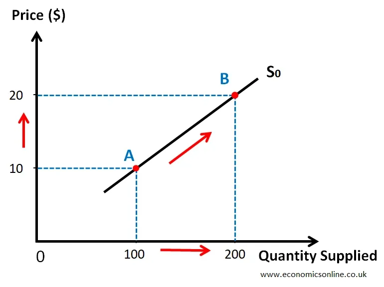
In the above supply curve, the quantity supplied of a good is taken on the X-axis (horizontal axis) and the price on the Y-axis (vertical axis). The upward sloping supply curve S0 shows the positive or direct relationship between the price of a good and its quantity supplied, ceteris paribus.
Movement along the Supply Curve
Movement along the same supply curve is caused by a change in the price of product. It can be an extension or a contraction in supply.
Extension in Supply
An increase in the quantity supplied of a good due to an increase in its price is called an extension in supply.
It is illustrated by the following diagram:
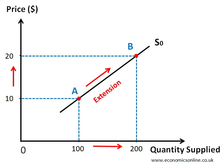
The movement from point A to point B is an extension in supply.
Contraction in Supply
A decrease in the quantity supplied of a good due to a decrease in its price is called a contraction in supply.
It is illustrated by the following diagram:
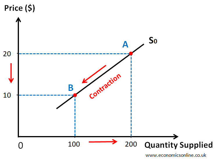
The movement from point A to point B is a contraction in supply.
Shift of the Supply Curve
A supply curve shifts due to a change in any non-price factor. The shifts in supply curves can be a rise or a fall in supply.
Rise in Supply
The rightward shift of the supply curve is called the rise in supply. It occurs when the whole supply schedule is increased due to a change in any non-price factor.
Fall in Supply
The leftward shift of the supply curve is called the fall in supply. It occurs when the whole supply schedule is decreased due to a change in any non-price factor.
The following diagram illustrates the rise and fall in supply.
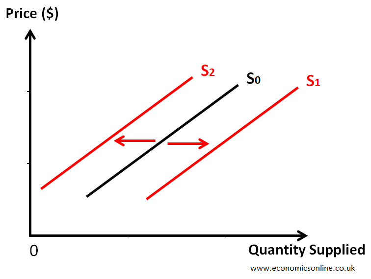
The rise in the supply curve is from S0 to S1, while the fall in the supply curve is from S0 to S2.
Factors Affecting Supply
There are many factors affecting the supply of a product in the market. Some of them are explained below.
Cost of Production
Firms consider their production costs, including labour, raw materials, and overhead expenses, which can affect the quantity they are willing to supply. An increase in the cost of production due to higher input prices, expensive utilities or higher prices of components can lead to a fall in the supply of a product and vice versa.
Technological Advances
Innovations and advancements in production methods can enhance efficiency, reduce costs, and increase the quantity that producers are willing to supply.
Resource Availability
The availability of key inputs or factors of production, such as natural resources and skilled labor, influences the production capacity and ultimately impacts the quantity supplied.
Government Policies
Government regulations, taxes, subsidies, and trade barriers can influence production costs and affect the quantity supplied by altering incentives for producers.
For more details, you can read the article on the supply shifters.
Price Elasticity of Supply (PES)
The degree of responsiveness of the quantity supplied of a good to the change in its price alone is called the price elasticity of supply.
Elastic supply implies that a small percentage change in price results in a large percentage change in quantity supplied, while inelastic supply indicates a small percentage change in quantity supplied in response to price changes.
Demand: Understanding the Behaviour of Consumers
Demand means the willingness and ability of buyers to buy different quantities of a good at various prices in a given time period, ceteris paribus. The word ceteris paribus means that all non-price factors are assumed to be constant.
Quantity Demanded
The quantity demanded is the number of units of a good which buyers are willing and able to buy at a specific price in a given time period, ceteris paribus.
The Law of Demand
The law of demand states that there is a negative or inverse relationship between price of a good and its quantity demanded, ceteris paribus.
The Demand Schedule
The demand schedule is a table which shows the negative or inverse relationship between the price of a good and its quantity demanded, ceteris paribus. Consider the following simple demand schedule:
|
P ($) |
Quantity Demanded |
|
20 |
100 |
|
10 |
200 |
In the above demand schedule, the left column shows a decrease in price while, the right column shows a corresponding increase in quantity demanded of a product. This shows the negative or inverse relationship between the price of a product and its quantity demanded, ceteris paribus.
Demand refers to the whole demand schedule and does not change when the price of the product changes. A change in the price of a good causes a change in its quantity demanded, while, a change in any non-price factor causes a change in demand.
The Demand Curve
The demand curve is a curve which shows a negative or inverse relationship between the price of a good and its quantity demanded, ceteris paribus. It is the graphical representation of the demand schedule. The following demand graph illustrates the demand curve based on the data in above table.
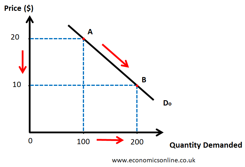
In the above demand curve, the quantity demand of a good is taken on X-axis (horizontal axis) and the price on the Y-axis (vertical axis). The downward sloping demand curve D0 shows the negative or inverse relationship between the price of a good and its quantity demanded, ceteris paribus. The normal demand curves have downward slopes.
Movement along the Demand Curve
Movement along the same demand curve is caused by a change in the price of product. It can be an extension or a contraction in demand.
Extension in Demand
An increase in the quantity demanded of a good due to a decrease in its price is called an extension in demand.
It is illustrated by the following diagram.
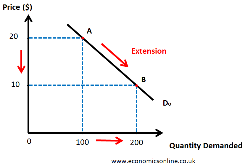
The movement from point A to point B is an extension in demand.
Contraction in Demand
A decrease in the quantity demanded of a good due to an increase in its price is called a contraction in demand.
It is illustrated by the following diagram.
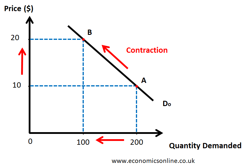
The movement from point A to point B is a contraction in demand.
Shift of the Demand Curve
Shift of the demand curve is caused by a change in any non-price factor. It can be a rise or a fall in demand.
Rise in Demand
The rightward shift of the demand curve is called the rise in demand. It occurs when the whole demand schedule is increased due to a change in any non-price factor.
Fall in Demand
The leftward shift of the demand curve is called the fall in demand. It occurs when the whole demand schedule is decreased due to a change in any non-price factor.
The following diagram illustrates the rise and the fall in demand.
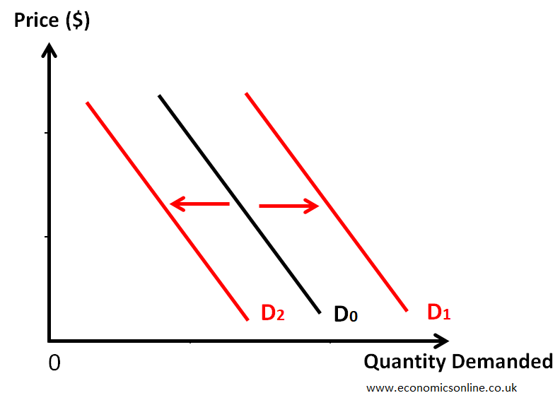
The rise in the demand curve is from D0 to D1, while the fall in the supply curve is from D0 to D2.
Factors Affecting Demand
There are many factors affecting the demand of a product in the market. Some of them are explained below.
Consumer Income
Changes in consumer income can influence demand due to changes in the purchasing power of consumers. For normal goods, an increase in income leads to higher demand, while for inferior goods, the opposite holds true.
Consumer Preferences
Individual tastes, preferences, and trends impact the demand for goods and services. Changing consumer preferences can result in shifts in demand for specific products.
Population Changes
Shifts in population size, demographic composition, and age distribution can affect the overall demand for goods and services in an economy.
Advertising
Advertising done by firms can change the demand of a product. For example, an advertising by a seller of flavoured milk may emphasise its health benefits and its demand will increase without a change in its price.
Prices of Related Goods
The change in the price of another good can also cause the shift in demand. For example, increase increase in the price of Pepsi can increase the demand for Coca Cola (Pepsi and Coca Cola are substitute goods). Like the prices of substitute goods, the change in the price of a complement can also shift the demand for a product.
Price Elasticity of Demand (PED)
The degree of responsiveness of the quantity demanded of a good to the change in its price alone is called the price elasticity of demand.
Elastic demand means that a small percentage change in price leads to a large percentage change in quantity demanded, while inelastic demand indicates a small percentage change in quantity demanded in response to price changes.
Market Equilibrium: Understanding the Interaction of Producers and Consumers
Market equilibrium occurs when the quantity supplied equals the quantity demanded at a particular price.
The intersection of the market supply curve and the market demand curve represents the equilibrium price and equilibrium quantity in the market. This is illustrated by the following diagram.
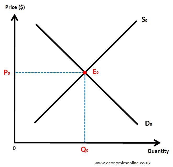
In above graph, the equilibrium point is E0 where the demand curve intersects the supply curve. P0 is the equilibrium price and Q0 is the equilibrium quantity.
Market Disequilibrium
Market disequilibrium occurs when the quantity supplied is not equal to the quantity demanded at a particular price. It can be a market surplus or a market shortage. When a surplus or shortage occurs, market forces and the price mechanism work to restore equilibrium.
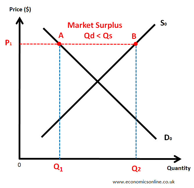
Market Surplus (Excess Supply)
When the quantity supplied exceeds the quantity demanded at a given price, a surplus occurs. This surplus puts downward pressure on prices, encouraging producers to decrease their output or adjust prices to clear the excess supply.
This is illustrated by the following graph.
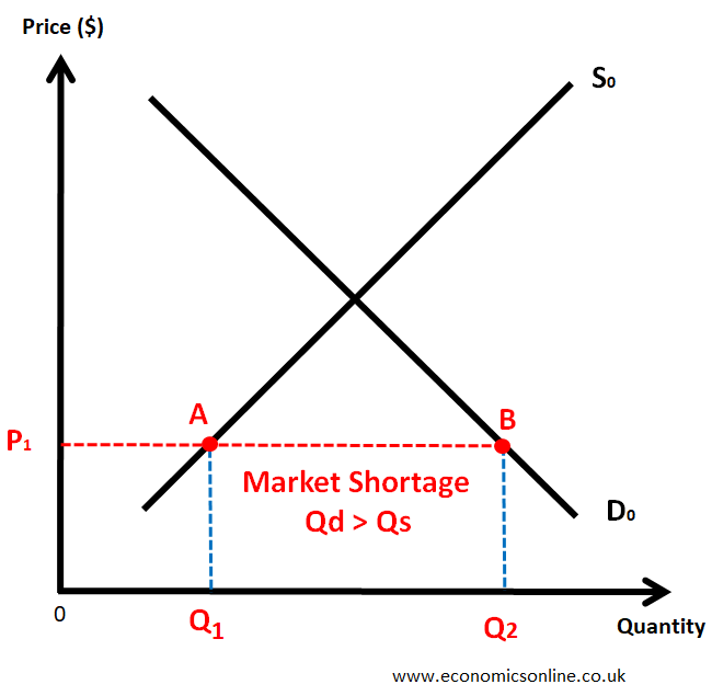
Market Shortage (Excess Demand)
When the quantity demanded exceeds the quantity supplied at a given price, a shortage arises. This shortage drives prices upward as consumers compete for limited supply, prompting producers to increase output or raise prices to meet the higher demand.
This is illustrated by the following graph.
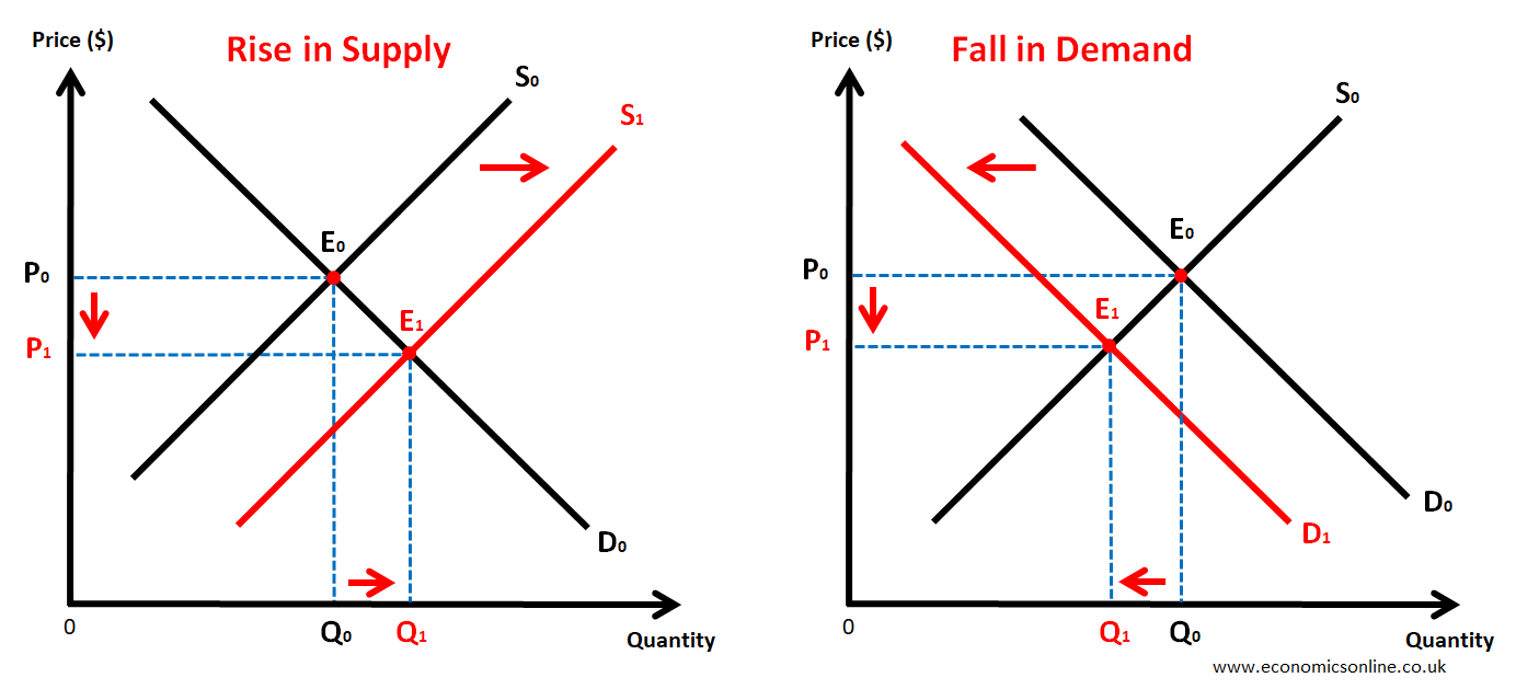
Changes in Market Equilibrium
Market equilibrium can change due to the shift in demand, the shift in supply or the simultaneous shift in the demand and the supply. After these shifts, a new equilibrium price (P1) and a new equilibrium quantity (Q1) is formed.
Conclusion
The supply and demand curves are fundamental concepts in economics and they are used to understand the behaviour of the consumers and the producers in the market of a commodity. These concepts are used by consumers, producers and the governments to make informed decisions.

