What is Quantization & Sampling? Types & Laws of Compression
What Is Quantization & Sampling? Types Of Quantization, What Is μ-Law & A-Law of Compression?
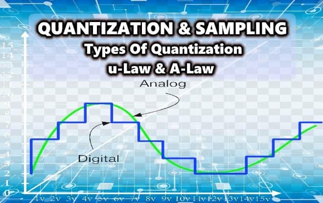
What Is Quantization?
Quantization is the process of mapping continuous amplitude (analog) signal into discrete amplitude (digital) signal.
The analog signal is quantized into countable & discrete levels known as quantization levels. Each of these levels represents a fixed input amplitude.
During quantization, the input amplitude is round off to the nearest quantized level. This rounding off is known as quantization error. Quantization error can be reduced by increasing the numbers of quantization levels.
Related Post: What is GSM and How does it Work?
Example Of Quantization
The figure below represents an analog signal. During quantization, the analog signal’s amplitude is sampled and discretized into fixed quantization levels.


In this example, we have used 8 quantization levels. The quantization results in the loss of information. The space between two adjacent levels is known as step size.
Step size = Vref/number of levels.
Vref represents the maximum amplitude being represented.
If the step-size is large then the quantization error will be high. In another word, the loss of information goes higher as the step size gets bigger.
Types Of Quantization
There are two types of quantization.
Uniform Quantization
The type of quantization in which the quantized levels are uniformly spaced is known as uniform quantization. In uniform quantization, each step size represents a constant amount of analog amplitude. it remains constant throughout the signal.
The example of uniform quantization is given below,
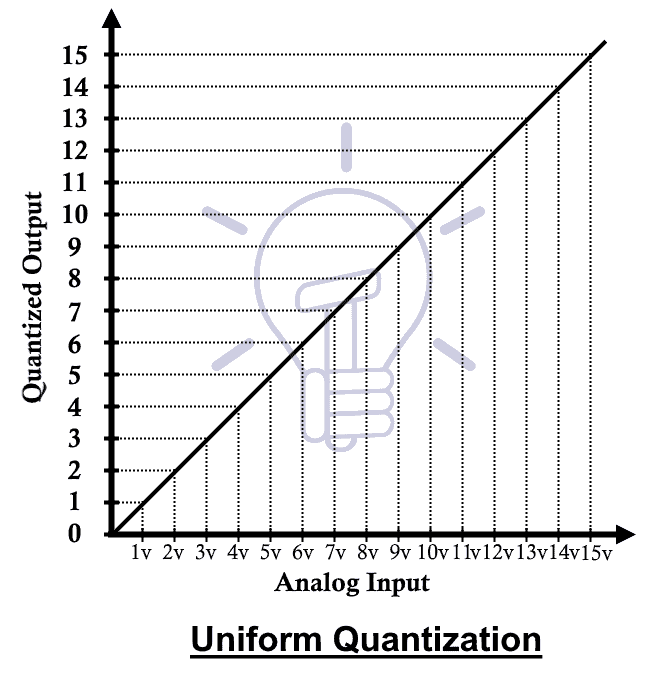
In this example, the space between any two adjacent step or levels represents 1-volt amplitude.
Non-Uniform Quantization
The type of quantization in which the space between the quantized levels is non-uniform & has logarithmic relation is called non-uniform quantization.
In non-uniform quantization, the analog signal is first passed through a compressor. The compressor applies a logarithmic function on the input signal. The input signal has a high difference between its low and high amplitude. In the output signal, the low amplitudes get amplified and the high amplitude levels get attenuated, Thus making a compressed signal.
Suppose the input signal’s amplitude is m & mp is the peak amplitude of the signal. Y is the output signal. Then the compression graph looks like:
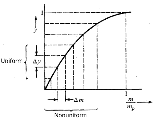
As you can see from the graph, that the small input levels Δm are mapped onto bigger output levels Δy. And the higher input levels are mapped onto smaller output levels.
- Related Post: What are Industrial Communication Networks? An Overview
There are two laws for compression
μ-Law
μ law is a compression algorithm used for non-uniform quantization. The expression of μ law is
y = (ln(1 + μ(m/mp)))/ (ln(1 + μ))

Where μ is the compression parameter and m is the input amplitude & mp is the peak amplitude of the input signal.
When μ=0, then there is no compression and the quantization becomes uniform. The characteristic graph for μ Law is given below:
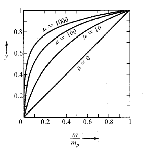
This graph shows that if the compression parameter μ is higher than the input signal is more compressed.
A-Law
A-law is another algorithm for compression of an analog signal for non-uniform quantization. The expression for A-law is:
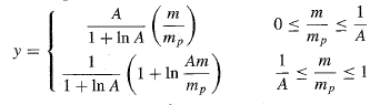
Where A is the compression parameter. When A=1, then the quantization is uniform because there is no compression. The characteristics graph is given below.
Both laws are applicable with some trade-offs.
Sampling
Sampling is an important step in analog to digital conversion. The taking or capturing of samples of input analog amplitude is called sampling.
Sampling Rate
The sampling rate is the number of samples taken in the duration of one second. it is measured in hertz or sample per second. The continuously varying amplitude of an analog signal is also continuous in time. So it needs to be sampled at a fixed rate. This rate is called sampling rate or sampling frequency. Example of sampling:
This signal is sampled at a sampling rate of 2 samples per second or 2 Hz.
Sampling rate plays important role in the perfect conversion from analog to digital and reconstruction of an analog signal from the digital signal.
Sampling rate should not be very low or very high. In both cases, the converted signal is not what we want to achieve. If the sampling rate is low than the original signal is destroyed and if the sampling rate is very high then it’s not economically beneficial.
Aliasing
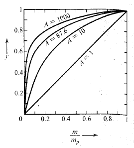
If the analog signal is sampled at a frequency lower than the required rate then the sampled signal does not appear to be anything like the original signal. And the reconstruction of the original signal becomes impossible. Such case is called aliasing as shown in the figure below.
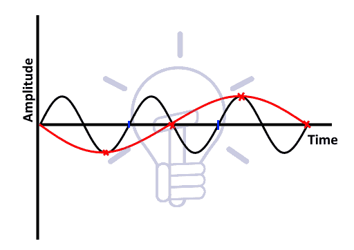
In this example, a sinusoidal signal is sampled at a rate of 3/4 of its frequency. which is very lower than its required rate. The reconstructed signal (red signal) is recovered from the sample which does not look anything like the original signal.
Nyquist Theorem
The sampling rate or sampling frequency should be greater than twice the input signal’s frequency. Nyquist theorem suggests the minimum sampling rate for a signal which can be perfectly reconstructed from its samples.
Related Posts
- Types of Control & Communication Cables
- What is Industrial Automation | Types of Industrial Automation
- Why Radio Waves Are Chosen For Close Range Transmission?
- Serial Communication by Arduino