Characterizing Nearshore Fish Assemblages From Intact and Altered Mangrove Shorelines in Biscayne Bay, Florida, United States

Introduction

Estuarine and coastal ecosystems are among the most exploited and threatened ecosystems (Worm et al., 2006; Barbier et al., 2011). Mangroves were historically replaced with filled land and gray coastal structures like seawalls to facilitate development throughout Florida. Human-altered structures may be physically replacing and existing among mangroves, but they do not fulfill the ecological functions and services of mangroves (Strain et al., 2018). Coastal developments and canals reduce and divide mangrove habitats, resulting in smaller habitat fragments which support fewer species (MacArthur and Wilson, 1963; Carugati et al., 2018). Seawall construction leads to the deterioration of coastal habitats, which affects the animal communities that rely on nearshore habitats for food sources and shelter (Prosser et al., 2018). Grey coastal structures lack the structural complexity of natural vegetation, thus reducing habitat niches, shelter, and refuge (Bulleri and Chapman, 2010; Loke and Todd, 2016; Schoonees et al., 2019). Even where artificial structures support fish assemblages, these assemblages do not resemble the assemblages of nearby natural shorelines (Chapman and Bulleri, 2003; Chapman and Underwood, 2011). Coastal structures can also affect the suitability of coastal habitats as reproductive and nursery grounds (Balouskus and Targett, 2012; Munsch et al., 2017).

Mangrove wetland systems are often impacted by alterations to the watershed intended to reduce flooding, which can make areas inhospitable to mangrove survival. Canals alter the hydrology of estuaries and may decrease freshwater flow, potentially increasing the salinity and the variability of salinity in coastal waters, thereby reducing estuarine habitats (Parker et al., 1955; Browder et al., 2005). Additionally, canals and marinas are both point sources of pollution (Browder et al., 2005). Canals can also release unnatural, stochastic freshwater pulses, nutrient-enriched agricultural runoff, landfill leachate, and polluted sediments into coastal waters (Browder et al., 2005; Caccia and Boyer, 2005). Submerged aquatic vegetation and benthic communities in South Florida are affected by canal discharge (Kohout and Kolipinski, 1967; Meeder et al., 1997; Meeder et al., 1999). Both canals and marinas involve dredging to create channels, some of which are deep enough for boat traffic. Dredging modifies and fragments the seafloor terrain, which is a significant driver of fish assemblage composition (Borland et al., 2022). Dredging also increases potentially toxic suspended sediment loads, which can affect fish physiology and reproduction, possibly resulting in increased mortality (Kjelland et al., 2015).

Mangrove wetland functions include generating biological productivity and diversity, absorbing nutrients and pollutants, stabilizing sediments, dissipating wind and wave energy, providing shelter for marine fauna, and serving as reproductive and nursery habitats (Barbier et al., 2011). Diverse and abundant fish assemblages are key indicators of a productive mangrove wetland system. Fish populations reflect the conditions and quality of marine systems in general, making them good indicators for detecting anthropogenic impacts (Munkittrick and Dixon, 1989; Izzo et al., 2016). Characterizing fish assemblages can reveal important information about the ecological functioning and environmental health of coastal wetlands. Historical and current fish assemblages can also be used to set conservation and restoration goals or metrics for success (Izzo et al., 2016).

Coastal fish species utilize mangrove ecosystems for feeding grounds, shelter, and refuge from predators. Resident fish may forage in mangrove systems, while other fish utilize mangroves for shelter and refuge during the day and forage elsewhere at night (Rooker and Dennis, 1991; Nagelkerken et al., 2000; Hammerschlag et al., 2010; Vaslet et al., 2012). Fish also use mangrove wetlands as nursery habitat which supports populations of adult fish in many other coastal habitats, including coral reefs (Nagelkerken, 2009; Jones et al., 2010). Mangrove wetland ecosystems make effective nurseries as they have ample food supplies, reduced predation pressure, and complex three-dimensional root structures, which provides juvenile fish with protection from potential predators (Beck et al., 2001; Laegdsgaard and Johnson, 2001). Many reef fish depend on mangroves for nursery habitats and are more speciose and abundant where mangrove extent is greater in the Caribbean (Nagelkerken et al., 2001; Nagelkerken et al., 2002; Serafy et al., 2015; Shideler et al., 2017).

Fish do not just rely on mangroves for habitat; they are critical components of the whole coastal ecosystem. Greater species richness increases morphological trait variation and interactions between species, which strengthens ecosystem processes and increases productivity (Loreau, 2000). Biodiversity improves the ability of an ecosystem to maintain multiple functions and increases their stability of functions during environmental fluctuations (Yachi and Loreau, 1999; Loreau et al., 2001; Maestre et al., 2012). Fish are an ecologically important taxon, fulfilling many ecosystem functions and services like regulating and linking functions, and cultural and information services (Holmlund and Hammer, 1999). As consumers, fish regulate trophic dynamics, thereby maintaining species and genetic biodiversity (Holmlund and Hammer, 1999). Fish also maintain ecosystem resilience, as functional diversity increases the stability of ecosystem processes (Chapin et al., 1997; Yachi and Loreau, 1999; Loreau et al., 2001; Maestre et al., 2012). Fish activity regulates sediment processes and nutrient cycles. Fish disrupt and resuspend sediments while foraging for benthic prey, burrowing, and spawning (Montgomery et al., 1996; Holmlund and Hammer, 1999). Bioturbation stirs up benthic invertebrate prey and nutrients which support phytoplankton growth (Breukelaar et al., 1994; Bilby et al., 1998; Adámek and Marsálek, 2013). Bioturbation also oxygenates sediments, which in turn increases phosphate and ammonia in the substrate entering the water (Brönmark and Hansson, 2005). Through excretion, fish increase nutrient enrichment and nitrogen availability to submerged aquatic vegetation, which boosts benthic primary productivity and herbivory (Peterson et al., 2013). Juvenile Haemulidae can excrete 0.04 – 0.06 µmol NH₄⁺ per mg of biomass each day; excretion increases with fish biomass, while excretory nutrient concentrations decrease as fish biomass increases (Meyer and Schultz, 1985).

Fish also provide linking services by connecting different components of the marine seascape. Fish represent all trophic levels and make energy and nutrients from vegetation and detritus available for other ecological trophic levels. Small and juvenile fish found in mangroves serve as food for larger fish, transporting carbon, nutrients, and energy up the food web. Fish move between adjacent habitats on a daily basis as they move with the tides, seek shelter, avoid predation, and forage for food (Rooker and Dennis, 1991; Nagelkerken et al., 2000; Krumme, 2009; Hammerschlag et al., 2010; Baker et al., 2013). Mangrove-associated fish frequently exhibit seasonal and ontogenetic migrations, as well (Rooker and Dennis, 1991; Jones et al., 2010). As fish move, they transport nutrients, carbon, and energy between habitats, thereby facilitating connectivity between marine ecosystems, which increases biodiversity and productivity (Holmlund and Hammer, 1999; Boström et al., 2011; Nagelkerken et al., 2015).

Fish also provide demand-derived ecosystem services, such as information and cultural services, which are valued based on our demand for them (Holmlund and Hammer, 1999). Individual fish, populations, and communities can provide information to scientists (Holmlund and Hammer, 1999). Fish populations can be used to assess the overall health, resilience, and functionality of an ecosystem (Öhman et al., 1998; Holmlund and Hammer, 1999). Fish are economically important, providing food and aquaculture, medicines, recreation, aesthetics, while reducing waste, algal blooms, and disease (Holmlund and Hammer, 1999). Florida saltwater recreational fishing generated $9.2 billion and supported 88,501 jobs annually, while saltwater commercial fisheries (includes invertebrates) generated $3.2 billion and supported 76,700 jobs in Florida annually (FWC, 2020). Fish also provide aesthetic and recreational values through fishing, scuba diving, snorkeling, tourism, and even the aquarium trade (Holmlund and Hammer, 1999). If coastal habitats are degraded and can no longer support nearshore fish populations, then coastal systems will no longer provide these ecosystem functions and services.

The largest threats to mangroves in Florida are urban, agricultural, and industrial development (Kruczynski and Fletcher, 2012). Over 80% of the mangrove wetlands in the Indian River Lagoon and the mangrove shoreline in Lake Worth along the Atlantic Coast of Florida have been lost or rendered functionally obsolete through impoundments (Kruczynski and Fletcher, 2012; Florida Department of Environmental Protection, 2021). Except for contiguous forests in Southwest Florida, most of the mangrove wetlands in Florida are limited to isolated fragments or thin strips along the shore with reduced buffering capabilities (Kruczynski and Fletcher, 2012). The degradation of coastal habitats has caused quantifiable declines in viable fisheries, loss of nursery habitats, and decreases in filtering and detoxifying services (Barbier et al., 2011).

Biscayne Bay is a very speciose component of the intensively used and highly managed South Florida ecoregion (Sullivan Sealey and Bustamante, 1999). Over 600 fish species have been reported in Biscayne National Park and over 120 species have been recorded in NOAA’s Integrated Biscayne Bay Ecological Assessment and Monitoring (IBBEAM) mangrove surveys since 1998. A healthy fish assemblage in Biscayne Bay would include diverse taxa, feeding guilds, and life history stages. In this paper, we utilized a large public dataset to characterize fish assemblages that are representative of mangrove shorelines in South and Central Biscayne Bay. Sites included both intact mangroves and mangrove shorelines that have been altered with drainage canals or small marinas. We expected that fish samples will form different assemblages, possibly associated with different mangrove shoreline types, with higher fish abundances in front of intact mangroves but greater species richness around altered mangroves. Our hypotheses were informed by a previous study by Peters et al. (2015) which found that intact mangrove shorelines and riprap-altered mangrove shorelines supported different fish assemblages, with greater species richness in front of riprap-mangroves shorelines and greater fish abundances and nursery functionality in front of intact mangrove shorelines. Habitat heterogeneity can increase functional and species diversity (Hajializadeh et al., 2020), so human-altered structures within mangrove forests may support greater fish diversity, provided that the alteration does not too severely impact environmental conditions.

Methods

Study Site: South and Central Biscayne Bay

Biscayne Bay is a shallow coastal lagoon on the Atlantic coast of South Florida and includes both marine and estuarine habitats (Roessler and Beardsley, 1974; Browder et al., 2005). Biscayne Bay is considered to have three ecological sections: North, Central, and South Biscayne Bay (Roessler and Beardsley, 1974; Browder et al., 2005; Caccia and Boyer, 2005; Caccia and Boyer, 2007). North Biscayne Bay stretches from Dumfoundling Bay to the Rickenbacker Causeway, while Central Biscayne Bay stretches from Rickenbacker Causeway to Featherbed Bank/Black Point, and South Biscayne Bay extends from Featherbed Bank/Black Point to Card Sound/Jewfish Creek (Caccia and Boyer, 2005).

In its natural state, the western shore of Biscayne Bay was dominated by mangrove wetlands with some saltmarsh wetlands (Roessler and Beardsley, 1974; Browder et al., 2005). Mangroves were removed, coastal wetlands filled in, and grey coastal structures were constructed to facilitate the rapid development of Miami in the 1900s (Cantillo et al., 2000). Biscayne Bay has lost approximately 80% of its mangrove wetland areas (Serafy et al., 2003). Biscayne Bay was previously hydrologically linked to the Everglades system through both aboveground and belowground water flow (Browder et al., 2005). Drainage canals were used to convert wetlands to dry land and to control flooding (Cantillo et al., 2000). However, diverting the flow of water in the Everglades reduced freshwater entering Biscayne Bay, affecting both the hydrology and ecology of the entire bay (Alleman and Black, 1995; Browder et al., 2005; Caccia and Boyer, 2005). With less freshwater input, salinities increased, salinity gradients changed, and marine communities replaced many estuarine communities (Parker et al., 1955; Browder et al., 2005; Kruczynski and Fletcher, 2012).

South Biscayne Bay is the least developed region of the Bay and is dominated by mangrove wetlands, but drainage canals fragment the mangroves and impact faunal communities (Browder et al., 2005; Caccia and Boyer, 2007). The southern portion of Central Biscayne Bay also has large mangrove wetlands intersected by canals and is similar to, but more developed than, South Biscayne Bay. South and Central Biscayne Bay provide equally suitable fish habitats (Bernal et al., 2014). Canals release unnatural freshwater pulses, nutrient-enriched agricultural runoff, landfill leachate, and polluted sediments into Biscayne Bay (Caccia and Boyer, 2005). Reduced freshwater inflow has lowered mangrove functionality, while associated saltwater intrusion has facilitated scrubland mangroves migrating into former freshwater wetlands (Browder et al., 2005). Submerged aquatic vegetation and benthic communities in South and Central Biscayne Bay are affected by canal discharge (Kohout and Kolipinski, 1967; Meeder et al., 1997; Meeder et al., 1999). Fish communities now lack estuarine species that were historically found in Biscayne Bay (Serafy et al., 2001; Udey et al., 2002; Browder et al., 2005).

Data Collection

All data used in this study was collected from South and the southern portion of Central Biscayne Bay by the IBBEAM Project (Southeast Fisheries Science Center, 2021). IBBEAM was established in 2012 to document water quality and faunal responses to the Comprehensive Everglades Restoration Plan along mangrove shorelines of Biscayne Bay. IBBEAM consolidated and standardized data collection for four preexisting independent programs, including the mangrove-associated fish surveys (Southeast Fisheries Science Center, 2021). As such, over 20 years of fish surveys from Biscayne Bay are publicly available online. Large public datasets allow ecologists to examine natural phenomena on larger spatial and temporal scales, while making the greatest use of existing information. The same large dataset can be used to answer different research questions, making it an efficient use of time and resources.

Beginning in 1998, mangrove-associated fish have been surveyed at approximately 50 different locations twice a year during the dry season (January to March) and the wet season (July to September) (Southeast Fisheries Science Center, 2021). Visual fish surveys were conducted along a 30-m-long and 2-m-wide belt transect (60 m² survey area) running parallel to the mangrove shoreline (Serafy et al., 2003; Southeast Fisheries Science Center, 2021). IBBEAM mangrove-associated fish surveys provided the abundance, minimum and maximum total lengths, and average total length for each fish taxa identified for each transect (Southeast Fisheries Science Center, 2021). The date, time, latitude and longitude, season, salinity, water depth, visibility (turbidity), water temperature, and dissolved oxygen were also recorded for each transect (Southeast Fisheries Science Center, 2021).

Six sites were selected in front of intact mangrove shorelines (Mang) and six sites were selected from altered mangroves (Alt) that contained a canal or marina. The six intact mangrove sites were selected as they each had approximately 20 IBBEAM transects from the last five years of available surveys in close proximity to each other. These sites were surrounded by the most intact mangrove shorelines and were all at least 1000 m away from the nearest coastal alteration, therefore representing the most natural areas. The six altered mangrove sites were selected because they also had about 20 IBBEAM transects from the last five years within 500 m of the alteration. These sites exhibited the greatest degree of human alteration, representing the least natural sites. To examine the current fish assemblages and avoid including temporal trends in fish assemblages, only the five most recent years of available surveys (2015 – 2019) were considered. This study utilized pre-collected large datasets, which limited site selection and resulted in an unequal latitudinal distribution as the four northern-most sites were all altered mangrove sites. This study design limited our ability to detect potential effects of shoreline type on fish assemblages. Details on each site can be found in Table 1, while a map of all the sites can be seen in Figure 1. Selected transect surveys with environmental data and fish abundances can be found in Supplementary Table 1.

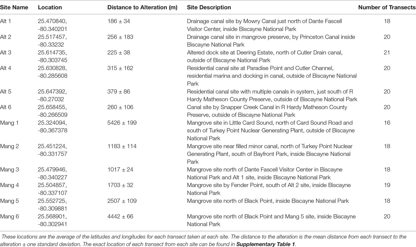
Table 1 The location, description, and sampling effort for each survey site.

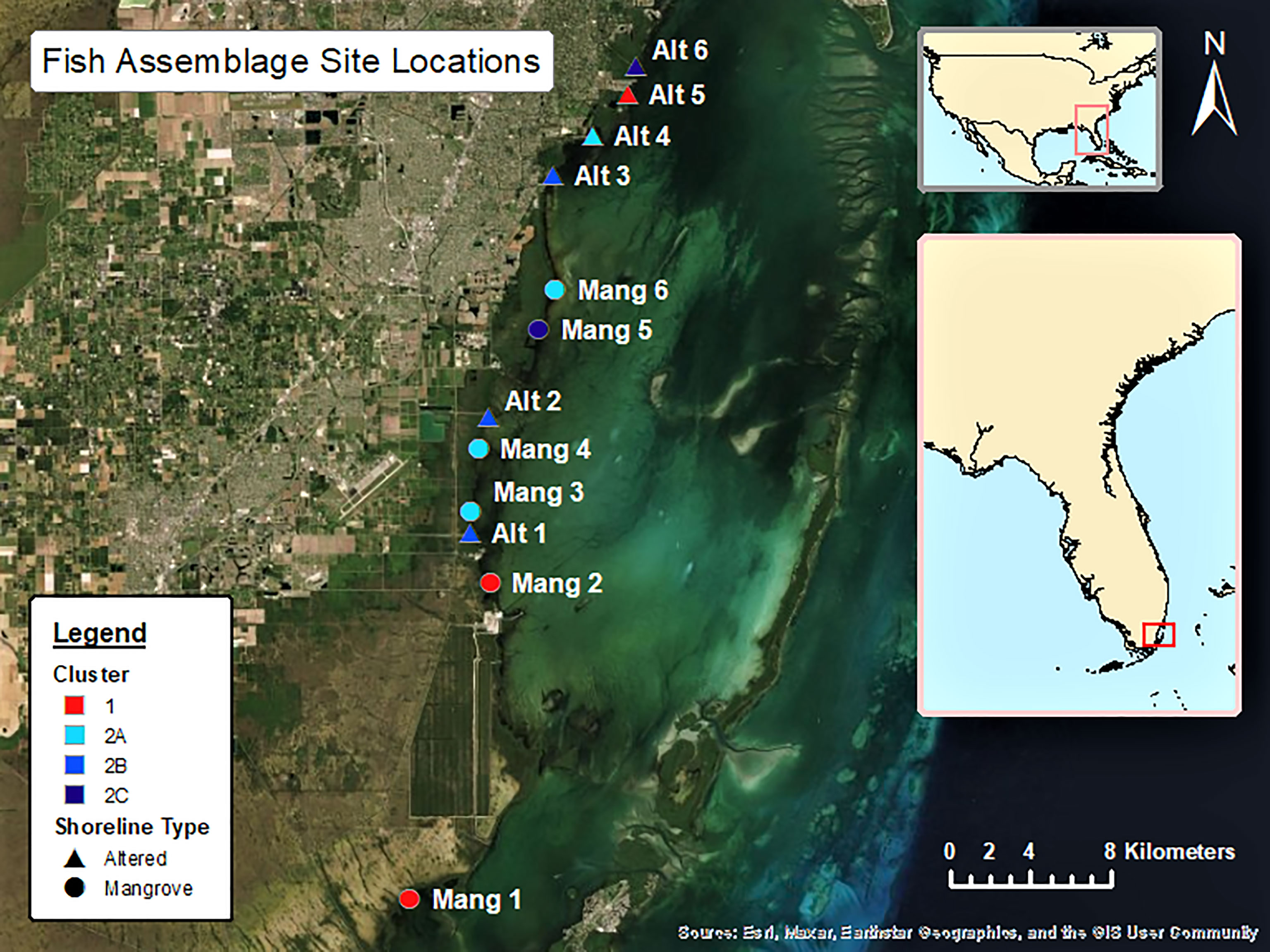
Figure 1 The 12 sites considered in the data analysis are in South and Central Biscayne Bay and stretch from Little Card Sound in the south to R Hardy Matheson County Preserve towards the north.

We were interested in examining fish assemblages from a larger ecological perspective that could indicate ecosystem functioning. Each transect provided a mere snapshot of the fish communities that were present at each site, so the fish counts from the transects were combined for each site to produce a representative sample which depicted the fish communities more accurately than using individual transects as samples could. Fish species were reported and discussed using scientific names; common names used in South Florida can be found in Supplementary Table 2. Small silver fish that often school together, such as Atherinidae, Clupeidae, and Engraulidae, were grouped into a single unit during IBBEAM surveys as they are difficult to distinguish to the species or family level in the field. Of the 56,599 total fish, 39,847 (70.4%) were small silver fish. These small silver fish were removed from the data for three reasons: (1) these fish were not identified to the family level, (2) removal of this group increased the normality of the whole dataset, and (3) these fish existed in high abundances across most sites which limited our ability to discriminate between assemblages based on other species.

Data Analysis

All statistical analyses were performed in RStudio using various packages. Based on the results of Shapiro-Wilk tests for normality, non-parametric Kruskal-Wallis tests were used to determine if water quality parameters were different between sites, shoreline types, and clusters. Both Shannon-Wiener (H’) and Simpson (D) diversity indices were calculated for each site using the vegan RStudio package (Oksanen et al., 2020). Pielou’s evenness was also calculated for each site. Fish abundance, species richness, diversity indices, and evenness indices were compared between intact and altered mangrove shorelines using a t-test.

All multivariate analyses were conducted twice: once on abundance data and then once on biomass data calculated from the mean lengths from a sample using the length-weight equation W = a L^b and constants (a and b) found on FishBase (2019). Both abundance and biomass data were fourth root transformed, as informed by heatmaps made with the ggplot2 RStudio package (Supplementary Figure 1) (Wickham, 2016). A Bray-Curtis dissimilarity matrix was created for all 12 sites using the vegan RStudio package (Oksanen et al., 2020). An analysis of similarity (ANOSIM) with 999 permutations in the RStudio vegan package was then conducted to determine if the sites within each shoreline type were more similar to each other than to sites from other shoreline types (Oksanen et al., 2020). Those results necessitated using the dissimilarity matrix to create an agglomerative hierarchical cluster analysis using the average method in the stats RStudio package, visualized with a dendrogram (R Core Team, 2021). A similarity profile (SIMPROF) analysis was then used to determine how many significant clusters were formed from the hierarchical cluster analysis using the clustsig RStudio package (Whitaker and Christman, 2014). Another ANOSIM with 999 permutations was then conducted to confirm that the sites within each cluster were more similar to each other than to sites in other clusters (Oksanen et al., 2020). Kruskal-Wallis tests were used to test for differences in water quality variables between clusters. Similarity percentage (SIMPER) analyses in the vegan RStudio package were then conducted on each possible pairing of clusters to determine which species most contributed to the dissimilarity in fish composition between the assemblages (Oksanen et al., 2020). SIMPER results were used to create a list of distinguishing species for each assemblage. To be considered a distinguishing species, it had to be one of the species responsible for 50% of the cumulative dissimilarity between cluster pairs. Each of those fish species were then designated as distinguishing species for whichever cluster from the pairwise comparison it had the highest abundance in.

The initial analysis warranted taking a closer look at a single cluster made up of nine of the 12 sites, so the aforementioned analyses were repeated on both abundance and biomass of those nine sites. A Bray-Curtis dissimilarity matrix was used to create an agglomerative hierarchical cluster analysis using the average method; these sub-clusters were then confirmed using an ANOSIM with 999 permutations (Oksanen et al., 2020; R Core Team, 2021). Following sub-cluster formation, all environmental variables were compared between sub-clusters using Kruskal-Wallis tests. SIMPER analyses were again conducted to determine which species most contributed to the dissimilarity in fish composition between the sub-clusters and to create a list of distinguishing fish species for each sub-cluster (Oksanen et al., 2020).

Distinguishing fish species of each cluster were then considered in terms of feeding guilds, trophic levels, and salinity tolerance (Supplementary Table 3). Mean trophic levels of distinguishing species were retrieved from FishBase and compared between assemblages using a Kruskal-Wallis test (FishBase, 2019). Reef-associated distinguishing species were also compared between Assemblage 1 and 2. Species data included size range, so total lengths of reef-associated fish were compared to the known lengths at sexual maturity to determine if the reef-associated fish in the mangrove habitats were juveniles or adults, which may indicate if any of the sites were nursery habitats. We were unable to determine the proportion of juveniles if many life history stages were present at a site. The average lengths of reef-associated species present as juveniles were compared between assemblages using a Kruskal-Wallis test.

Finally, non-metric multidimensional scaling (NMDS) plots were created using the vegan and ggplot2 RStudio packages to show how similar the fish composition of sites were (Wickham, 2016; Oksanen et al., 2020). NMDS plots also visualized how the sites clustered into distinct fish assemblages. The NMDS plots were overlaid with the intrinsic fish species which may be driving the site distribution pattern and with the extrinsic environmental variables correlated with the distribution pattern.

Results

A total of 16,752 individuals from 36 different fish species (or broader taxonomical units) and 24 different families were included in the data analyses. Several fish species are shown in Figure 2 and a full species list can be found in Supplementary Table 2. The eight most abundant species accounted for nearly 95% of the total fish abundance: Eucinostomus spp. (44.79% of total abundance), Floridichthys carpio (16.43%), Gerres cinereus (16.06%), Lutjanus griseus (11.07%), Abudefduf saxatilis (1.82%), Haemulon sciurus (1.65%), Sphyraena barracuda (1.49%), and Lutjanus apodus (1.27%). The other 28 species each contributed less than 1.00% to the total fish abundance. The eight species with the greatest biomass accounted for 87.71% of total biomass: L. griseus (46.17% of total), G. cinereus (18.46%), S. barracuda (8.90%), H. sciurus (4.66%), Centropomus undecimalis (3.89%), Eucinostomus spp. (2.23%), Mugil cephalus (1.83%), and L. apodus (1.56%).

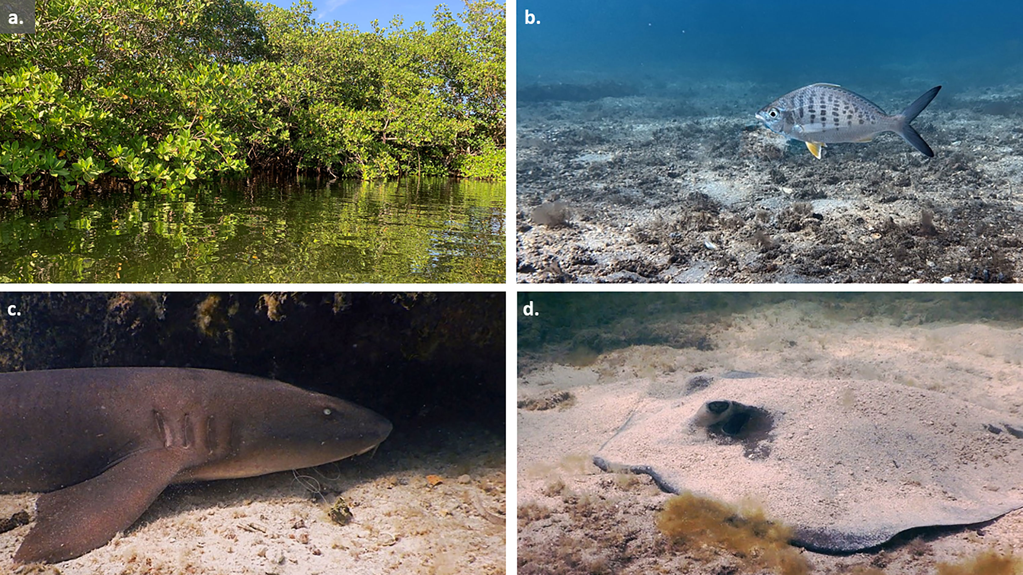
Figure 2 (A) The mangrove shoreline as seen from site Alt 5, photo credit Ellery Lennon. (B) Gerres cinereus were among the most abundant fish seen in the IBBEAM surveys, photo credit Ellery Lennon. (C) Ginglymostoma cirratum, photo credit Maria Laukaitis, and (D) Hypanus americanus, photo credit Kathleen Sullivan Sealey, were among the least abundant fish seen during the IBBEAM surveys.

Sites

Many environmental parameters differed between sites and shoreline types. Salinity varied by site (H = 104.52, df = 11, p < 2.2e-16); higher and more stable salinities were found in the southernmost and northernmost sites, while sites in the middle of the latitudinal range exhibited lower and more variable salinities. Salinity also differed between shoreline types (H = 10.226, df = 1, p = 0.001385) and was slightly higher in altered mangrove sites. Water depth also varied by site (H = 76.848, df = 11, p = 5.983e-12) and exhibited a similar pattern as salinity; the southernmost and northernmost sites were slightly deeper than the central sites. Depth was also greater in altered mangrove (Alt) than intact mangrove (Mang) sites (H = 4.3071, df = 1, p-value = 0.03795). Visibility varied across sites (H = 45.702, df = 11, p = 3.649e-06). Visibility was different between shoreline types (H = 15.259, df = 1, p-value = 9.371e-05) and was greater in front of intact mangrove sites. Recorded temperatures and dissolved oxygen levels did not differ across sites (H = 4.938, df = 11, p = 0.934 and H = 7.462, df = 11, p = 0.761, respectively) or between shoreline types (H = 1.2468, df = 1, p-value = 0.2642 and H = 0.065675, df = 1, p-value = 0.7977, respectively).

Five of the six intact mangrove sites were more speciose and diverse than five of the six altered sites. The exceptions were site Alt 5 which was the most diverse site, and Mang 5 which had the second-lowest diversity. While intact mangrove sites had higher average species richness, Shannon-Wiener Diversity, Simpson Diversity, and Pielou’s Evenness values than altered sites, and altered sites had higher average fish abundances, these trends were not significant (Table 2). There was not a statistically significant difference in total fish abundance (t = 0.848, p = 0.417), species richness (W = 10.5, p-value = 0.252), Shannon-Wiener Diversity (t = -0.793, p = 0.446), Simpson Diversity (t = -0.718, p = 0.489), or Pielou’s Evenness (t = -1.224, p = 0.249) between altered and intact mangrove shorelines. Fish species composition did not differ significantly between shoreline types (abundance ANOSIM R = -0.033, p = 0.597; biomass ANOSIM R = -0.057, p = 0.691).

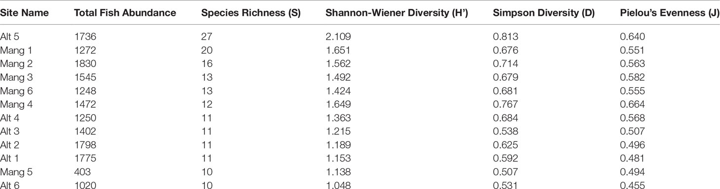
Table 2 Univariate species richness, diversity, and evenness of each site. Sites are ordered by species richness in descending order.

Characterizing Fish Assemblages

The 12 sites formed two main clusters, one of which was further divided into three sub-clusters. The same clusters were produced from both abundance data and biomass data, although the exact relationship between sites varied slightly. The two main clusters (“Cluster 1” and “Cluster 2”) were significantly different per an ANOSIM (abundance ANOSIM R = 0.892, p = 0.006; biomass ANOSIM R = 0.941, p = 0.004). Cluster 1 contained three sites: Mang 1, Mang 2, and Alt 5. Cluster 2 contained the other nine sites: Mang 3, Mang 4, Mang 5, Mang 6, Alt 1, Alt 2, Alt 3, Alt 4, and Alt 6. Because Cluster 2 contained most of the sites, a cluster analysis and ANOSIM were performed on those nine sites separately to determine sub-clusters. Cluster 2 was subsequently split into three sub-clusters (abundance ANOSIM R = 0.7, p = 0.001; biomass ANOSIM R = 0.7, p = 0.003). Cluster 2A contained sites Mang 3, Mang 4, Mang 6, and Alt 4; Cluster 2B has sites Alt 1, Alt 2, and Alt 3, while Cluster 2C was formed from sites Mang 5 and Alt 6 (Figure 3).

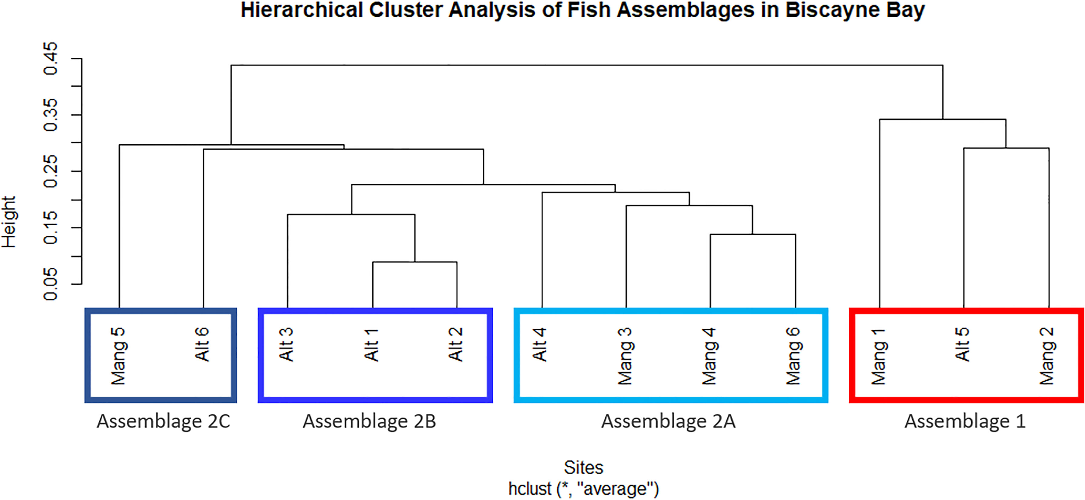
Figure 3 Clusters of distinct fish assemblages based on fish abundance data. Two primary clusters were formed, then Cluster 2 was split into three additional sub-clusters. These clusters are interpreted as ecologically significant species assemblages.

There did not seem to be any trends in seascape or latitude between Clusters 1 and 2, as they both contained intact and altered sites, sites inside and outside of Biscayne National Park, and covered a wide latitudinal range within the study area. The three sub-clusters formed from Cluster 2 did not appear to correlate with latitude (an overall distance of about 25 km). Assemblage 2A (Mang 3, Mang 4, Mang 6, Alt 4) consisted of mostly intact mangrove sites that are inside Biscayne National Park, but still contained one residential canal site outside of the park. Assemblage 2B (Alt 1, Alt 2, Alt 3) consisted of only altered sites, two of which are within the boundaries of Biscayne National Park, while Alt 3 is just north of the park. Assemblage 2C (Mang 5, Alt 6) consisted of one altered site outside Biscayne National Park and one intact mangrove site in Biscayne National Park.

Salinity was different between Clusters 1 and 2 (H = 36.850, df = 1, p = 1.276e-09); Cluster 1 salinities were higher and less variable than those measured at sites in Cluster 2. Salinity also varied between Clusters 2A, 2B, and 2C (H = 6.375, df = 2, p = 0.041) and was highest in Cluster 2C. Water depth also differed as sites in Cluster 1 were slightly deeper than Cluster 2 (H = 11.970, df = 1, p = 0.001), but depth did not vary between Clusters 2A, 2B, and 2C (H = 2.374, df = 2, p = 0.305). Cluster 1 sites had greater visibility and water clarity than Cluster 2 (H = 21.666, df = 1, p = 3.245e-06); visibility did not differ between Clusters 2A – 2C (H = 2.302, df = 2, p = 0.316). Temperature was not different between clusters (H = 0.789, df = 1, p = 0.375 for Cluster 1 and 2; H = 0.556, df = 2, p-value = 0.757 for Clusters 2A – 2C). Additionally, dissolved oxygen did not vary between Clusters 1 and 2 (H = 0.055, df = 1, p = 0.815) or between Clusters 2A – 2C (H = 1.930, df = 2, p = 0.381) (Figure 4).

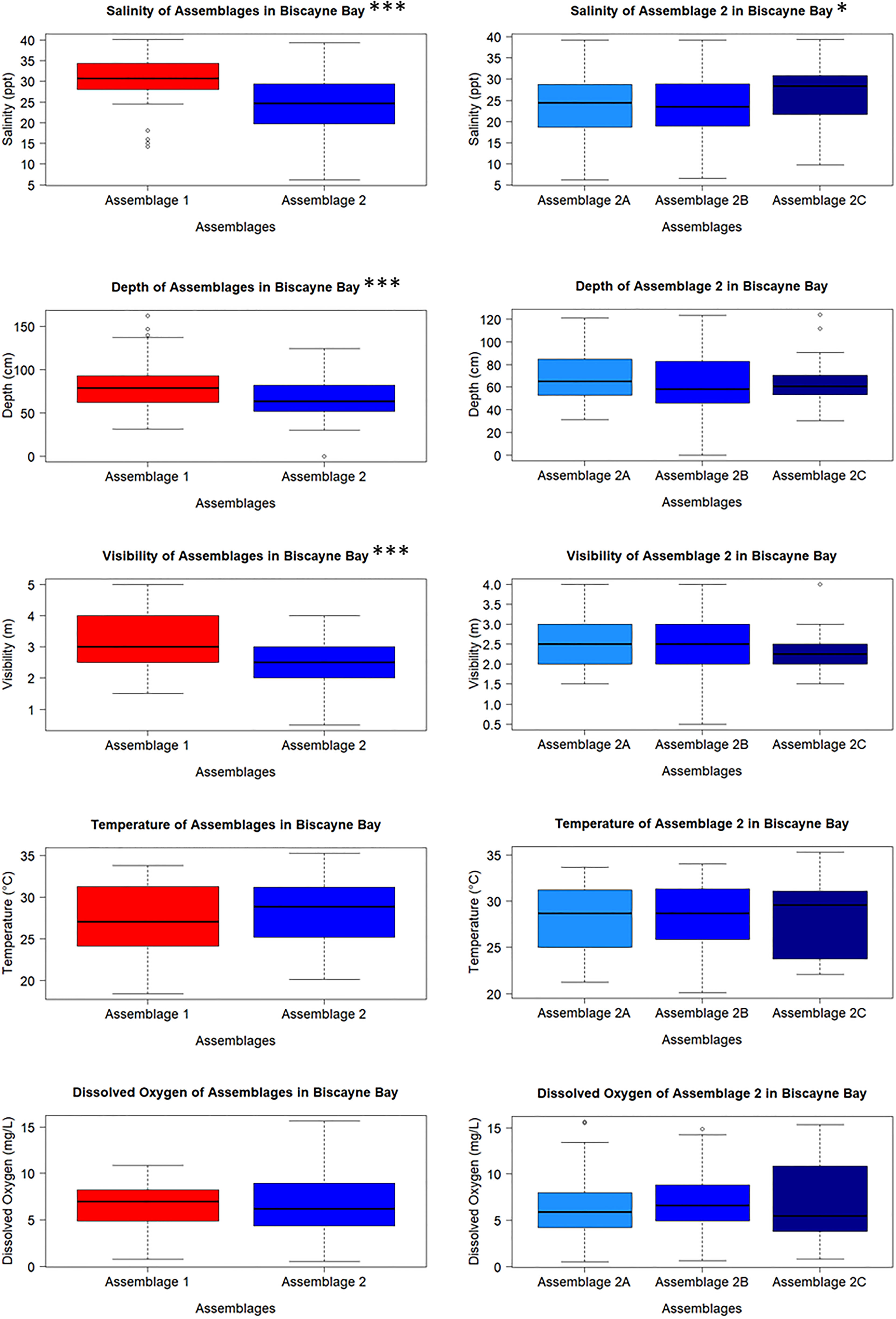
Figure 4 Water quality parameters taken from each sampling event from the sites that make up each cluster. Salinity differed between Clusters 1 and 2, and between Clusters 2A – 2C, while depth and visibility only differ between Clusters 1 and 2. Temperature and dissolved oxygen did not differ between any of the clusters. Significance levels: *** = 0.001; ** = 0.01; * = 0.05.

The three sites in Cluster 1 had the greatest species richness and above average diversity and evenness indices. Cluster 1 had many unique fish species: Haemulon parra, Scarus guacamaia, Anisotremus virginicus, Kyphosus sectatrix, Parablennius marmoreus, Lophogobius cyprinoides, Ginglymostoma cirratum, Lutjanus cyanopterus, Aetobatus narinari, Selene vomer, Sparisoma chrysopterum, Hypanus americanus, Mycteroperca bonaci, Lutjanus jocu, and Sparisoma rubripinne. However, many of these unique fish were observed at low abundances. A few fish species were unique to Cluster 2: Poecilia latipinna and Lucania parva were seen at several sites, while unidentified Gobiidae spp., Sphoeroides spengleri, invasive Mayaheros urophthalmus, and Lobotes surinamensis were at only one or two sites. The most abundant fish in Cluster 1 were L. griseus and Eucinostomus spp., while Eucinostomus spp. and F. carpio were the most abundant in Cluster 2 (Figure 5). The species with the greatest biomass were L. griseus and Eucinostomus spp. in Cluster 1 and G. cinereus, followed by L. griseus in Cluster 2 (Figure 6). Clusters were interpreted as ecologically significant fish assemblages with unique composition and will be referred to as “assemblages” for the remainder of the paper.

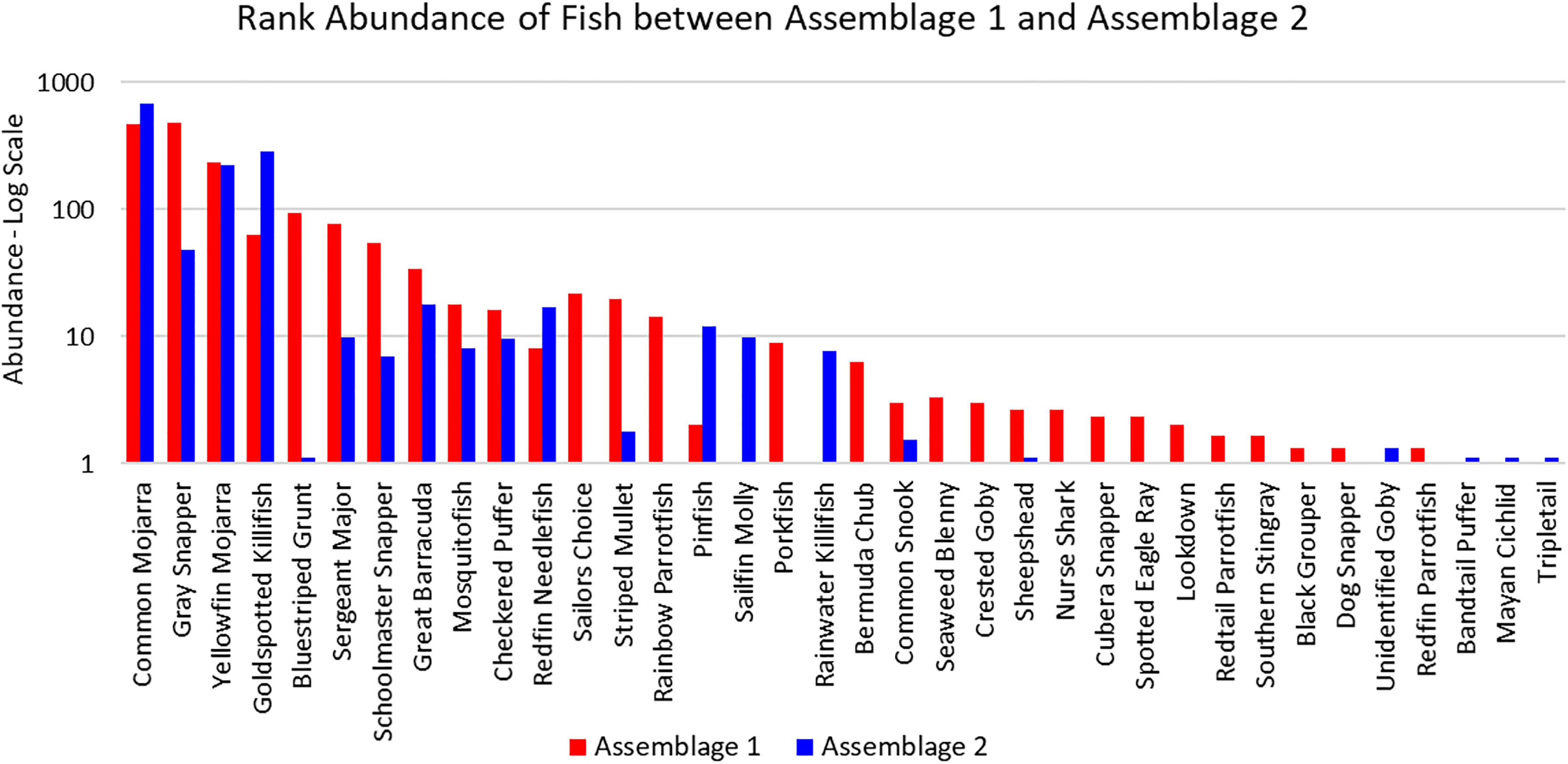
Figure 5 Ranked abundance of fish species found in Assemblages 1 and 2. The abundances are averaged by the number of sites forming each assemblage and shown on a log scale.

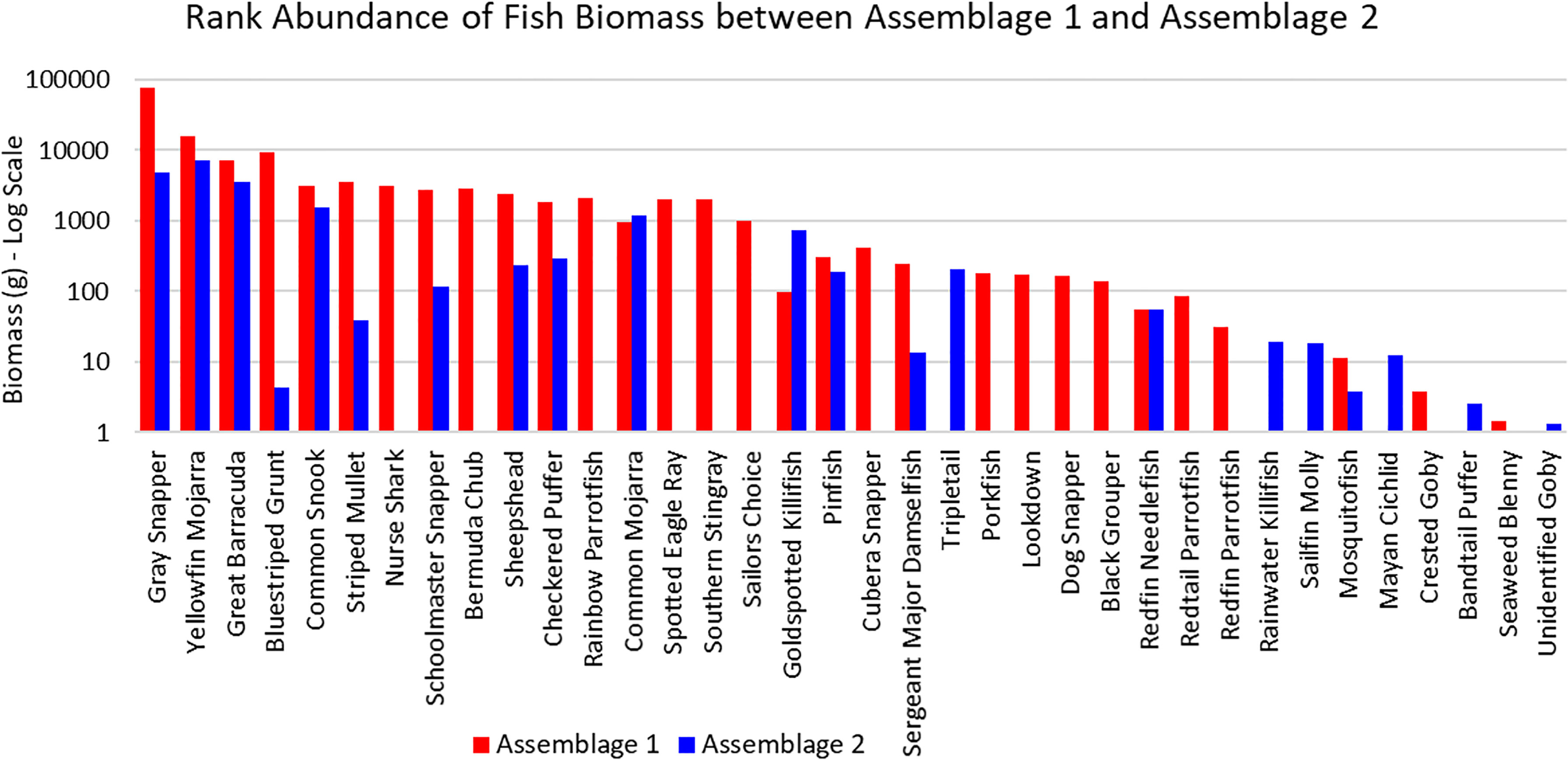
Figure 6 Ranked biomass of fish species found in Assemblages 1 and 2. The biomasses are averaged by the number of sites forming each assemblage and shown on a log scale.

According to the SIMPER analysis, both abundant and less abundant species were responsible for dissimilarity between Assemblages 1 and 2. The 50% of the dissimilarities in fish abundance between Assemblage 1 and 2 were due to H. sciurus, L. griseus, H. parra, F. carpio, A. saxatilis, A. virginicus, L. parva, S. guacamaia, L. apodus, and Gambusia spp. The 50% of the dissimilarities in biomass between Assemblage 1 and 2 were due to H. sciurus, L. griseus, C. undecimalis, H. parra, G. cirratum, S. guacamaia, H. americanus, Archosargus probatocephalus, and M. cephalus. Distinguishing species for Assemblages 1 and 2 are listed in Table 3.

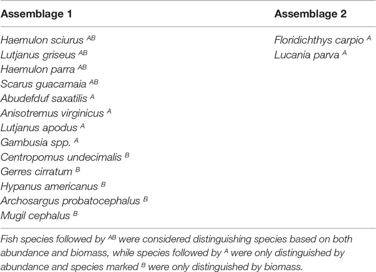
Table 3 Fish species that distinguished Assemblages 1 and 2 from each other, based on the SIMPER results and abundances/biomass of fish species.

Assemblage 2A (Mang 3, Mang 4, Mang 6, Alt 4) was characterized by higher diversity and evenness values than Assemblages 2B and 2C. P. latipinna, Gambusia spp., M. cephalus, H. sciurus, and M. urophthalmus were found only in Assemblage 2A, not in Assemblage 2B or 2C. Gobiidae spp., S. spengleri, and L. surinamensis were unique to Assemblage 2B. A. probatocephalus was the only species found in Assemblage 2C, but not in 2A or 2B. The most abundant species in both Assemblage 2A and 2B was the Eucinostomus spp., followed by the F. carpio. The most abundant species in Assemblage 2C were the Eucinostomus spp. and G. cinereus(Figure 7). G. cinereus and L. griseus contributed most to biomass in Assemblages 2A and 2B, while C. undecimalis and G. cinereus contributed most to biomass in Assemblage 2C (Figure 8).

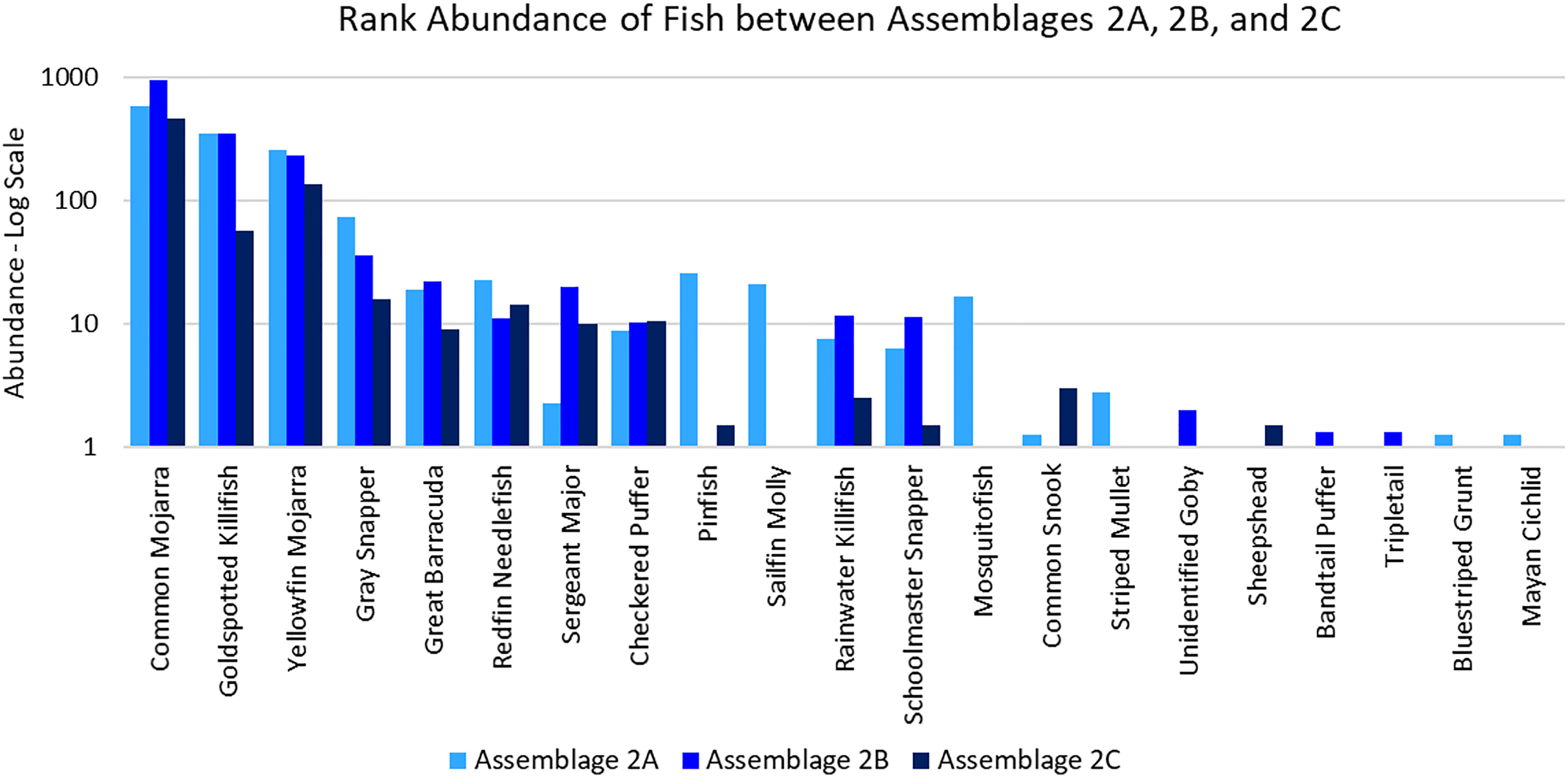
Figure 7 Ranked abundance of fish species found in Assemblages 2A, 2B, and 2C. The abundances are averaged by the number of sites forming each assemblage and shown on a log scale.

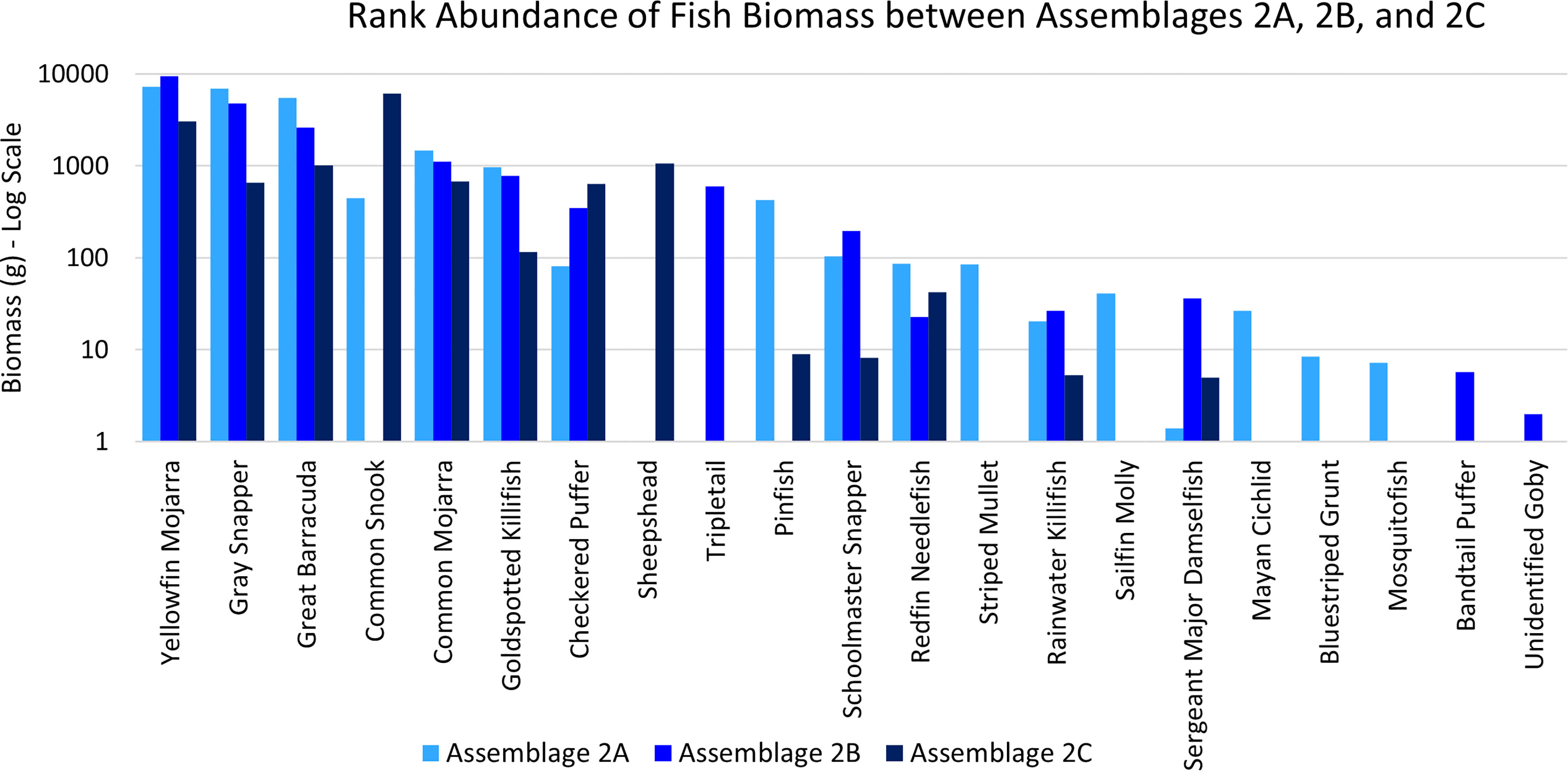
Figure 8 Ranked biomass of fish species found in Assemblages 2A, 2B, and 2C. The biomasses are averaged by the number of sites forming each assemblage and shown on a log scale.

According to the SIMPER analysis, both abundant and less abundant species were responsible for dissimilarity between Assemblages 2A, 2B, and 2C. The 50% of the dissimilarity in fish abundance between Assemblages 2A and 2B were due to Gambusia spp., P. latipinna, A. saxatilis, Lagodon rhomboides, L. griseus, and Strongylura notata forsythia. The 50% of the dissimilarity in fish biomass between Assemblages 2A and 2B were due to L. griseus, L. rhomboides, L. surinamensis, S. barracuda, P. latipinna, C. undecimalis, and A. saxatilis. The fish species responsible for 50% of the dissimilarities between Assemblages 2A and 2C were Gambusia spp., F. carpio, A. saxatilis, G. cinereus, P. latipinna, and S. notata forsythia. The fish responsible for 50% of the dissimilarities in biomass between Assemblages 2A and 2C were C. undecimalis, L. griseus, A. probatocephalus, G. cinereus, S. barracuda, and L. rhomboides. The 50% of the dissimilarity between Assemblages 2B and 2C caused by fish abundance was due to F. carpio, L. apodus, G. cinereus, S. notata forsythia, L. parva, and Eucinostomus spp. The 50% of the dissimilarity in biomass between Assemblages 2B and 2C were due to C. undecimalis, G. cinereus, L. griseus, A. probatocephalus, and L. apodus. These distinguishing species can be seen in Table 4.

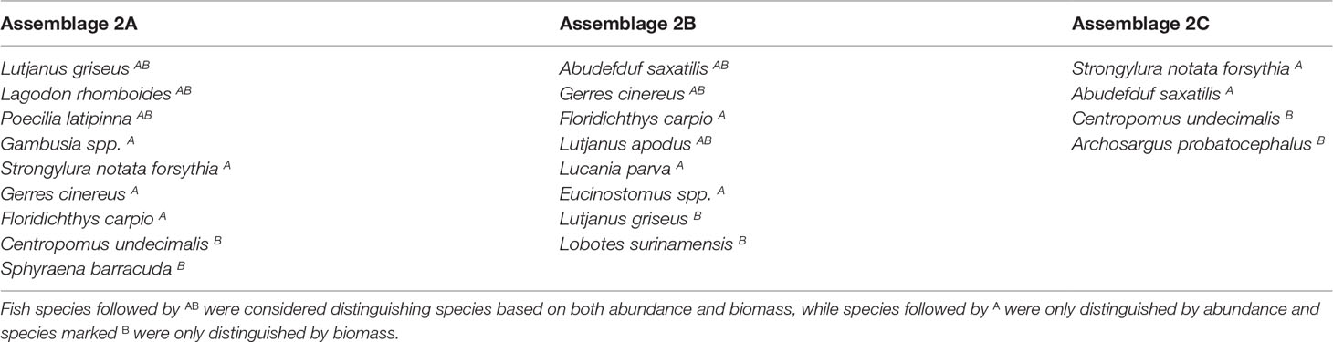
Table 4 List of species that distinguished each Assemblages 2A, 2B, and 2C from each other, based on the SIMPER results and abundances and biomass of fish species.

When examining distinguishing fish species from each assemblage in terms of feeding guilds, all clusters were dominated by invertivores and invertivore combinations, such as invertivore/piscivores. Ten out of the 13 distinguishing fish in Assemblage 1 were invertivores or invertivore combinations and both distinguishing fish in Assemblage 2 were planktivore/invertivores. While Assemblage 1 supported greater species richness, all feeding guilds were still present in Assemblage 2. There did not appear to be a difference in feeding guild representation between Assemblages 1 and 2, and trophic levels of distinguishing species did not differ between them (H = 0.749, df = 1, p = 0.387). Assemblages 2A, 2B, and 2C were also dominated by invertivore and invertivore combinations, however Assemblage 2A had the greatest feeding guild variety with herbivores, piscivores, and planktivores in addition to invertivores. Trophic levels of distinguishing species did not vary between Assemblages 2A, 2B, and 2C (H = 1.449, df = 2, p = 0.485).

While salinity did vary between clusters, fish did not appear to organize into clusters based on their salinity tolerances. Assemblage 1 did contain fish distinguishing species that were only considered marine, but most of the distinguishing species between Assemblage 1 and 2, and between Assemblages 2A, 2B, and 2C, had very wide ranges of salinity tolerances.

Ten of the observed fish species were reef-associated; five of these species were found only in Assemblage 1 and five were found in both Assemblages 1 and 2. G. cirratum, A. virginicus, S. guacamaia, H. parra, and H. americanus were only found in Assemblage 1. H. sciurus, L. griseus, S. barracuda, L. apodus, and A. saxatilis were found in both assemblages, but all of them were more abundant in Assemblage 1 than Assemblage 2 when averaged over the number of sites per assemblage. Average fish total lengths (TL) for each transect were used to determine the approximate size of reef-associated fish forming each assemblage (Figure 9). L. griseus (H = 10.644, df = 1, p = 0.001), S. barracuda (H = 9.453, df = 1, p = 0.002), L. apodus (H = 4.849, df = 1, p = 0.028), and A. saxatilis (H = 13.369, df = 1, p = 0.0003) were all shorter in Assemblage 2.

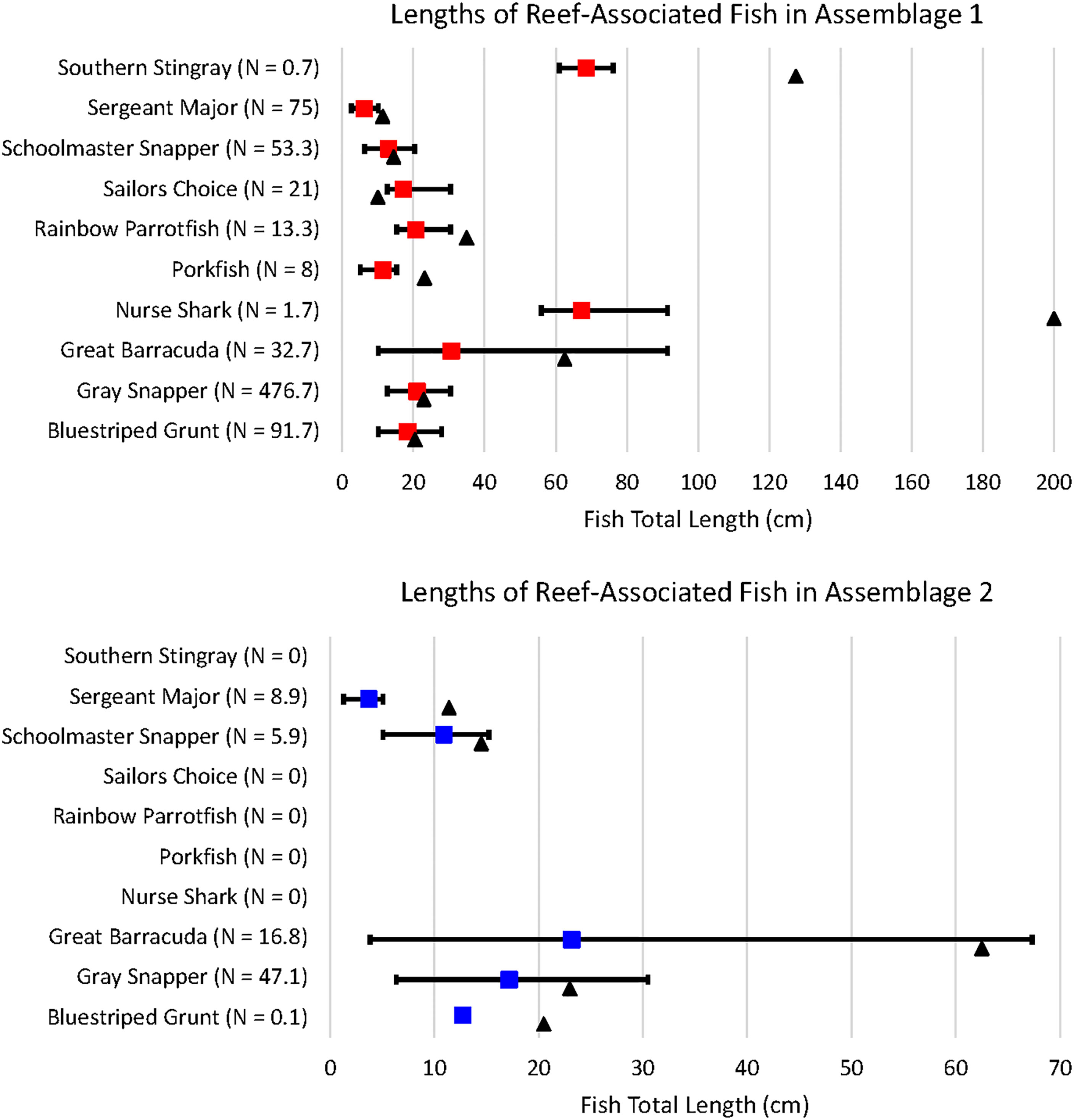
Figure 9 Nine of the ten reef-associated species were present as juveniles; sailors choice were only observed as adults. N denotes the mean number of individuals recorded per site. The colored squares denote the mean length, while the black triangle represents the length at maturity. A table showing the minimum, maximum, and average total lengths of fish in each assemblage, as well as the length at maturity for each species can be found in Supplementary Table 4.

Many of the H. sciurus in Assemblage 1 were juveniles and the only H. sciurus in Assemblage 2 was a juvenile, as well. Both juvenile and adult L. griseus, S. barracuda, and L. apodus were found in Assemblages 1 and 2. All A. saxatilis observed in both assemblages were juveniles. Of the five reef-associated species only found in Assemblage 1, G. cirratum, A. virginicus, S. guacamaia, and H. americanus were all juveniles, while all of the H. parra were adults.

Both the abundance and biomass NMDS plots supported the cluster analyses and indicated which environmental factors may be driving species composition. Fish assemblage ordination for both fish abundance and biomass were associated with mean salinity and mean depth of each sampling event (Figure 10). Mean salinity and mean depth were higher in Assemblage 1 than in Assemblage 2. Water temperature, dissolved oxygen, visibility, latitude, and shoreline alteration were not significantly associated with ordination. The lack of association between latitude and assemblage clustering validated our site selection.

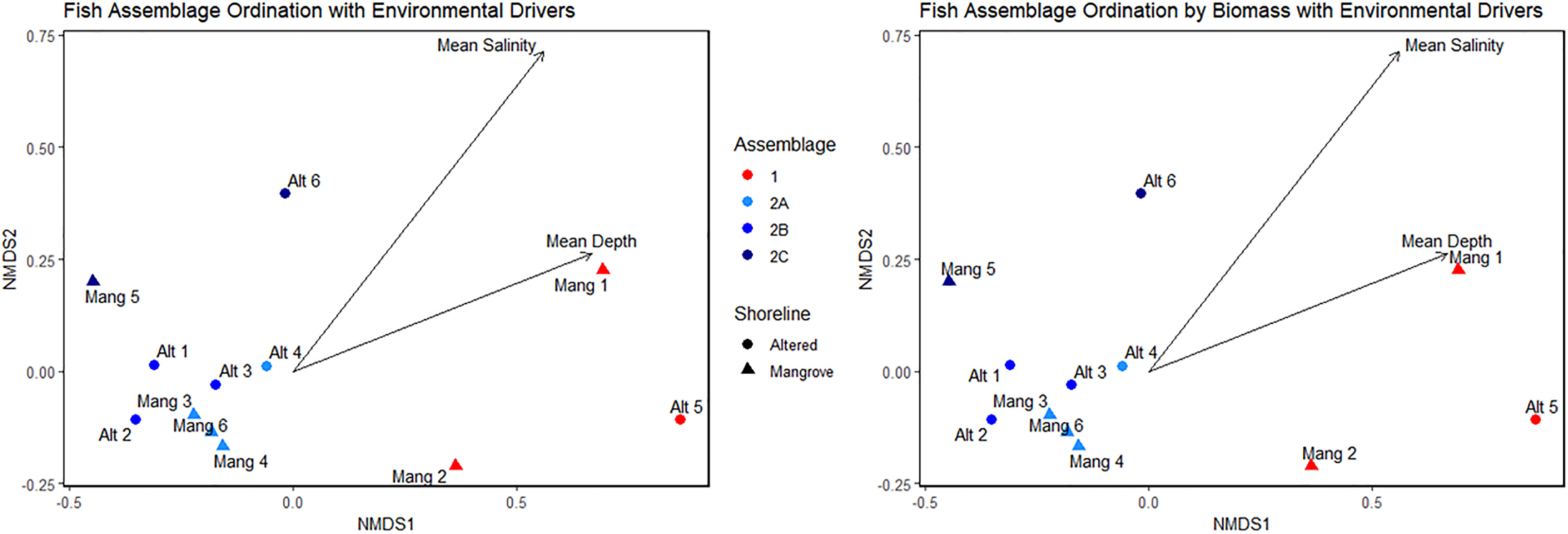
Figure 10 NMDS plots showing site ordinations forming distinct assemblages based on abundance and biomass with extrinsic environmental parameters overlayed on the plots.

Discussion

Fish formed distinct assemblages with different species composition that were ecologically meaningful, showing that cluster analyses are an appropriate methodology for statistically differentiating between fish assemblages. Two main assemblages with distinct fish composition, Assemblages 1 and 2, were found. Assemblage 2 was further divided into three sub-clusters, Assemblages 2A, 2B, and 2C. Assemblage 1 had the most species, higher average diversity and evenness indices, greater average abundances, and had more than twice the number of unique fish species as Assemblage 2. Assemblage 1 contained more species and greater abundances of reef-associated fish that were present as juveniles than Assemblage 2. Thus, sites in Assemblage 1 likely had higher quality environmental conditions and conferred greater ecosystem functions, including nursery functionality, than sites in Assemblage 2 (Munkittrick and Dixon, 1989; Yachi and Loreau, 1999; Loreau et al., 2001; Maestre et al., 2012; Izzo et al., 2016). Within Assemblage 2, Assemblage 2A had greater fish diversity and more unique species than Assemblages 2B and 2C. Assemblage 1, followed by Assemblage 2A, represented the healthiest assemblages in a highly managed, mangrove-dominated watershed and can be used to set goals and expectations following shoreline restoration in Central and North Biscayne Bay.

Salinity and depth measurements collected during surveys were correlated with assemblage formation, making them potential drivers of fish assemblages. Temperature and dissolved oxygen were relatively consistent between sites, so their lack of correlation does not correspond to a lack of importance for fish assemblages. Assemblage 1 was associated with higher salinities and greater depths, making it the “marine assemblage.” Altered mangroves had greater salinities and depths than intact mangrove sites, perhaps a consequence of dredging. Though these water quality parameters were associated with fish assemblages, shoreline type was not. Additionally, Assemblage 1 included two intact mangrove sites and one altered mangrove site. The water quality parameters collected at the sites at the time of the fish transect surveys are an incomplete picture of the Biscayne Bay water quality, and only provide an indication of conditions at the time of sampling. A more complete picture of the water quality trends is provided in other publications. Water quality in Biscayne Bay is extremely dynamic with active freshwater discharge management, characterized in other long-term studies (Caccia and Boyer, 2005; Stalker et al., 2009).

While Assemblage 1 was more diverse and this diversity confers greater functionality, Assemblage 1 does not represent the “natural” fish assemblage as Biscayne Bay has undergone significant hydrological changes over the past century. The environmental conditions of Biscayne Bay have shifted from estuarine to marine salinity regimes. Assemblage 1 could be used as guideposts to set expectations for future fish assemblages following shoreline restoration that results in higher and more stable salinities. Assemblage 2, on the other hand, is associated with lower and more variable salinities, making it the “estuarine assemblage”. Assemblage 2 may be representative of sites in Biscayne Bay following hydrology restoration that decrease salinities in nearshore waters.

Fish diversity and assemblages were not correlated with mangrove shoreline alterations, contradicting our initial hypothesis that intact and altered mangrove shorelines would support different fish assemblages. The presence of canals and residential marinas did not appear to cause differences in fish assemblages at this scale (10s of kilometers). This has positive implications for coastal restoration as mangrove shorelines in South and Central Biscayne Bay are still capable of supporting diverse fish assemblages. Some degree of shoreline alteration did not affect the surrounding mangroves’ ability to support fish assemblages similar to those found in nearby intact mangroves. The level of alteration at these sites was relatively minor compared to much of the Miami urban shorelines in Central and North Biscayne Bay, so this conclusion cannot be extended beyond South and southern Central Biscayne Bay.

Globally, mangrove loss and alteration are associated with declines in fish diversity and abundance. Mangrove conversion to aquaculture ponds in Thailand has been linked to declines in fish biomass and fisheries productivity (Naylor et al., 2000; Barbier, 2003). Mangrove deforestation unrelated to aquaculture is also associated with changing fish assemblage composition, lower species richness, lower fish abundances, and reduced fisheries yield (Fondo and Martens, 1998; Shinnaka et al., 2007). At the regional level, Caribbean fisheries and mangrove extent are declining at similar rates (Ellison and Farnsworth, 1996). Thus, there is likely a threshold at which alteration begins to noticeably change the ecology of fish assemblages. This does indicate that, below the aforementioned threshold, mangrove quality is not the main factor that drives fish assemblages. Mangrove extent cannot be the only factor considered in shoreline restoration because salinity and depth are correlated with distinct fish assemblage formation.

Mangrove extent, hydrology, and coastal geomorphology should all be considered in future restoration plans. Although we did not find a significant effect of shoreline alterations on fish, larger coastal alterations negatively impact fish diversity and assemblages (Bilkovic and Roggero, 2008; Henderson et al., 2019). Moving forward with climate change, sea level rise, and resilience, it is important to know how to maximize ecosystem performance. Understanding drivers of diverse fish assemblages in South and Central Biscayne Bay can help clarify the needs of shoreline restoration and mitigation in the more urban northern half of Biscayne Bay. Characterizing fish assemblages can set benchmarks for future alterations and both shoreline and hydrological restoration. These diverse fish assemblages from mangrove shorelines in South Biscayne Bay set a “best possible” goal for future fish assemblages following restoration in Central and North Biscayne Bay.

The Biscayne Bay watershed is complex and will be further altered by climate change (Wachnicka and Wingard, 2017), increasing the need for adaptive management. Biscayne Bay is going to undergo changes associated with the Comprehensive Everglades Restoration Plan and with further coastal alterations to mitigate flooding and quickly direct storm water runoff into the Bay. The Comprehensive Everglades Restoration Plan is focused on restoring the flow of freshwater from Lake Okeechobee south through the Everglades and into Florida and Biscayne Bays, which would change the salinity regimes back to estuarine. Biscayne Bay requires constant monitoring and the ability of management plans to shift with changing realities and needs. It is imperative that a balance is struck between coastal alterations offering flood resilience and with living shorelines to maintain ecological functions.

Data Availability Statement

The original contributions presented in the study are included in the article/Supplementary Material. Further inquiries can be directed to the corresponding author.

Ethics Statement

Ethical review and approval was not required for the animal study because we did not collect this data. The data analyzed was taken from a publicly available dataset from NOAA’s National Marine Fisheries Service.

Author Contributions

EL retrieved the data, conducted analyses, prepared the figures, and led the writing. KSS conceptualized the project and assisted with the writing. All authors contributed to the article and approved the submitted version.

Funding

This project was funded by the College of Arts and Science, University of Miami with research support to EL and KSS.

Conflict of Interest

The authors declare that the research was conducted in the absence of any commercial or financial relationships that could be construed as a potential conflict of interest.

Publisher’s Note

All claims expressed in this article are solely those of the authors and do not necessarily represent those of their affiliated organizations, or those of the publisher, the editors and the reviewers. Any product that may be evaluated in this article, or claim that may be made by its manufacturer, is not guaranteed or endorsed by the publisher.

Acknowledgments

We would like to acknowledge NOAA’s Integrated Biscayne Bay Ecological Assessment and Monitoring Project as our data source. IBBEAM data is publicly available and was retrieved online from https://www.fisheries.noaa.gov/inport/item/57694. We would also like to thank lab mate Jacob Patus for his assistance in making our site map (Figure 1).

Supplementary Material

The Supplementary Material for this article can be found online at: #https://www.frontiersin.org/articles/10.3389/fmars.2022.894663/full#supplementary-material

References

Adámek Z., Marsálek B. (2013). Bioturbation of Sediments by Benthic Macroinvertebrates and Fish and its Implication for Pond Ecosystems: A Review. Aquacult. Int. 21, 1−17. doi: 10.1007/s10499-012-9527-3
Alleman R. W., Black D. W. (1995). An Update of the Surface Water Improvement and Management Plan for Biscayne Bay (West Palm Beach, FL, US: South Florida Water Management District, Planning Department).
Baker R., Fry B., Rozas L. P., Minello T. J. (2013). Hydrodynamic Regulation of Salt Marsh Contributions to Aquatic Food Webs. Mar. Ecol. Prog. Ser. 490, 37–52. doi: 10.3354/meps10442
Balouskus R. G., Targett T. E. (2012). Egg Deposition by Atlantic Silverside, Menidia Menidia: Substrate Utilization and Comparison of Natural and Altered Shoreline Type. Estuaries Coasts 35 (4), 1100–1109. doi: 10.1007/s12237-012-9495-x
Barbier E. B. (2003). Habitat-Fishery Linkages and Mangrove Loss in Thailand. Contemp. Econom. Policy 21 (1), 59. doi: 10.1093/cep/21.1.59
Barbier E. B., Hacker S. D., Kennedy C., Koch E. W., Stier A. C., Silliman B. R. (2011). The Value of Estuarine and Coastal Ecosystem Services. Ecol. Monogr. 81 (2), 169–193. doi: 10.1890/10-1510.1
Beck M. W., Heck K. L., Able K. W., Childers D. L., Eggleston D. B., Gillanders B. M., et al. (2001). The Identification, Conservation, and Management of Estuarine and Marine Nurseries for Fish and Invertebrates: A Better Understanding of the Habitats That Serve as Nurseries for Marine Species and the Factors That Create Site-Specific Variability in Nursery Quality Will Improve Conservation and Management of These Areas. Bioscience 51 (8), 633–641. doi: 10.1641/0006-3568(2001)051[0633:TICAMO]2.0.CO;2
Bernal N. A., DeAngelis D. L., Schofield P. J., Sealey K. S. (2014). Predicting Spatial and Temporal Distribution of Indo-Pacific Lionfish (Pterois Volitans) in Biscayne Bay Through Habitat Suitability Modeling. Biol. Invasions 17 (6), 1603–1614. doi: 10.1007/s10530-014-0819-6
Bilby R. E., Fransen B. R., Bisson P. A., Walter J. K. (1998). Response of Juvenile Coho Salmon (Oncorhynchus Kisutch) and Steelhead (Oncorhynchus Mykiss) to the Addition of Salmon Carcasses to Two Streams in Southwestern Washington, USA. Can. J. Fish. Aquat. Sci. 55 (8), 1909–1918. doi: 10.1139/f98-094
Bilkovic D. M., Roggero M. M. (2008). Effects of Coastal Development on Nearshore Estuarine Nekton Communities. Mar. Ecol. Prog. Ser. 358, 27–39. doi: 10.3354/meps07279
Borland H. P., Gilby B. L., Henderson C. J., Connolly R. M., Gorissen B., Ortodossi N. L., et al. (2022). Dredging Fundamentally Reshapes the Ecological Significance of 3D Terrain Features for Fish in Estuarine Seascapes. Landscape Ecol., 1385−1400. doi: 10.1007/s10980-021-01394-5
Boström C., Pittman S. J., Simenstad C., Kneib R. T. (2011). Seascape Ecology of Coastal Biogenic Habitats: Advances, Gaps, and Challenges. Mar. Ecol. Prog. Ser. 427, 191–217. doi: 10.3354/meps09051
Breukelaar A. W., Lammens E. H., Breteler J. G. K., Tatrai I. (1994). Effects of Benthivorous Bream (Abramis Brama) and Carp (Cyprinus Carpio) on Sediment Resuspension and Concentrations of Nutrients and Chlorophyll a.Freshwater Biology.32, 1, 113–121. doi: 10.1111/j.1365-2427.1994.tb00871.x
Brönmark C., Hansson L.-A. (2005). The Biology of Lakes and Ponds (New York, NY, US: Oxford University Press).
Browder J. A., Alleman R., Markley S., Ortner P., Pitts P. A. (2005). Biscayne Bay Conceptual Ecological Model. Wetlands 25 (4), 854. doi: 10.1672/0277-5212(2005)025[0854:BBCEM]2.0.CO;2
Bulleri F., Chapman M. G. (2010). The Introduction of Coastal Infrastructure as a Driver of Change in Marine Environments. J. Appl. Ecol. 47 (1), 26–35. doi: 10.1111/j.1365-2664.2009.01751.x
Caccia V. G., Boyer J. N. (2005). Spatial Patterning of Water Quality in Biscayne Bay, Florida as a Function of Land Use and Water Management. Mar. pollut. Bull. 50 (11), 1416–1429. doi: 10.1016/j.marpolbul.2005.08.002
Caccia V. G., Boyer J. N. (2007). A Nutrient Loading Budget for Biscayne Bay, Florida. Mar. pollut. Bull. 54 (7), 994–1008. doi: 10.1016/j.marpolbul.2007.02.009
Cantillo A. Y., Pikula L., Hale K. K., Collins E. V., Caballero R. (2000). “Biscayne Bay Environmental History and Annotated Bibliography”, in National Status and Trends Program for Marine Environmental Quality (Silver Springs, Maryland: National Oceanic and Atmospheric Administration).
Carugati L., Gatto B., Rastelli E., Lo Martire M., Coral C., Greco S., et al. (2018). Impact of Mangrove Forests Degradation on Biodiversity and Ecosystem Functioning. Sci. Rep. 8 (1), 13298. doi: 10.1038/s41598-018-31683-0
Chapin F. S., Walker B. H., Hobbs R. J., Hooper D. U., Lawton J. H., Sala O. E., et al. (1997). Biotic Control Over the Functioning of Ecosystems. Science 277 (5325), 500–504. doi: 10.1126/science.277.5325.500
Chapman M. G., Bulleri F. (2003). Intertidal Seawalls—New Features of Landscape in Intertidal Environments. Landscape Urban Plann. 62 (3), 159–172. doi: 10.1016/S0169-2046(02)00148-2
Chapman M. G., Underwood A. J. (2011). Evaluation of Ecological Engineering of “Armoured” Shorelines to Improve Their Value as Habitat. J. Exp. Mar. Biol. Ecol. 400 (1), 302–313. doi: 10.1016/j.jembe.2011.02.025
Southeast Fisheries Science Center (2021). Mangrove Study Data ( NOAA National Centers for Environmental Information). Available at: https://www.fisheries.noaa.gov/inport/item/10678.
Ellison A. M., Farnsworth E. J. (1996). Anthropogenic Disturbance of Caribbean Mangrove Ecosystems: Past Impacts, Present Trends, and Future Predictions. Biotropica 28 (4), 549–565. doi: 10.2307/2389096
FishBase (2019). Available at: https://fishbase.us/ (Accessed October 15, 2021).
Florida Department of Environmental Protection (2021) Florida’s Mangroves. Available at: https://floridadep.gov/rcp/rcp/content/floridas-mangroves (Accessed February 1, 2022).
Fondo E. N., Martens E. E. (1998). Effects of Mangrove Deforestation on Macrofaunal Densities, Gazi Bay, Kenya. Mangroves Salt Marshes 2 (2), 75–83. doi: 10.1023/A:1009982900931
FWC (2020)The Economic Impacts of Saltwater Fishing in Florida. In: Florida Fish and Wildlife Conservation Commission. Available at: https://myfwc.com/conservation/value/saltwater-fishing/ (Accessed April 23 2021).
Hajializadeh P., Safaie M., Naderloo R., Shojaei M. G., Gammal J., Villnäs A., et al. (2020). Species Composition and Functional Traits of Macrofauna in Different Mangrove Habitats in the Persian Gulf. Front. Mar. Sci. 7 (809). doi: 10.3389/fmars.2020.575480
Hammerschlag N., Heithaus M. R., Serafy J. E. (2010). Influence of Predation Risk and Food Supply on Nocturnal Fish Foraging Distributions Along a Mangrove–Seagrass Ecotone. Mar. Ecol. Prog. Ser. 414, 223–235. doi: 10.3354/meps08731
Henderson C. J., Gilby B. L., Schlacher T. A., Connolly R. M., Sheaves M., Flint N., et al. (2019). Contrasting Effects of Mangroves and Armoured Shorelines on Fish Assemblages in Tropical Estuarine Seascapes. ICES J. Mar. Sci. 76 (4), 1052–1061. doi: 10.1093/icesjms/fsz007
Holmlund C. M., Hammer M. (1999). Ecosystem Services Generated by Fish Populations. Ecol. Econom. 29 (2), 253–268. doi: 10.1016/s0921-8009(99)00015-4
Izzo C., Doubleday Z. A., Grammer G. L., Gilmore K. L., Alleway H. K., Barnes T. C., et al. (2016). Fish as Proxies of Ecological and Environmental Change. Rev. Fish. Biol. Fish. 26 (3), 265–286. doi: 10.1007/s11160-016-9424-3
Jones D. L., Walter J. F., Brooks E. N., Serafy J. E. (2010). Connectivity Through Ontogeny: Fish Population Linkages Among Mangrove and Coral Reef Habitats. Mar. Ecol. Prog. Ser. 401, 245–258. doi: 10.3354/meps08404
Kjelland M. E., Woodley C. M., Swannack T. M., Smith D. L. (2015). A Review of the Potential Effects of Suspended Sediment on Fishes: Potential Dredging-Related Physiological, Behavioral, and Transgenerational Implications. Environ. Syst. Decisions 35 (3), 334–350. doi: 10.1007/s10669-015-9557-2
Kohout F. A., Kolipinski M. C. (1967). Biological zonation related to groundwater discharge along the shore of Biscayne Bay, Miami, Florida. In: Lauff, G. (ed.) Estuaries. Am. Assoc. Adv. Sci. Publ. No. 83, Washington, D.C.,488–499.
Kruczynski W. L., Fletcher P. J. (2012). Tropical Connections (Cambridge, MD, US: IAN Press, University of Maryland Center for Environmental Science).
Krumme U. (2009). “Diel and Tidal Movements by Fish and Decapods Linking Tropical Coastal Ecosystems,” in Ecological Connectivity Among Tropical Coastal Ecosystems (Dordrecht, Netherlands: Springer), 271–324.
Laegdsgaard P., Johnson C. (2001). Why do Juvenile Fish Utilise Mangrove Habitats? J. Exp. Mar. Biol. Ecol. 257 (2), 229–253. doi: 10.1016/S0022-0981(00)00331-2
Loke L. H., Todd P. A. (2016). Structural Complexity and Component Type Increase Intertidal Biodiversity Independently of Area. Ecology 97 (2), 383–393. doi: 10.1890/15-0257.1
Loreau M. (2000). Biodiversity and Ecosystem Functioning: Recent Theoretical Advances.Oikos. 91, 1, 3–17. doi: 10.1034/j.1600-0706.2000.910101.x
Loreau M., Naeem S., Inchausti P., Bengtsson J., Grime J., Hector A., et al. (2001). Biodiversity and Ecosystem Functioning: Current Knowledge and Future Challenges. Science 294 (5543), 804–808. doi: 10.1126/science.1064088
MacArthur R. H., Wilson E. O. (1963). An Equilibrium Theory of Insular Zoogeography. Evolution 17 (4), 373–387. doi: 10.1111/j.1558-5646.1963.tb03295.x
Maestre F. T., Quero J. L., Gotelli N. J., Escudero A., Ochoa V., Delgado-Baquerizo M., et al. (2012). Plant Species Richness and Ecosystem Multifunctionality in Global Drylands. Science 335 (6065), 214–218. doi: 10.1126/science.1215442
Meeder J., Alvord J., Byrne M., Ross M., Renshaw A. (1997). “Distribution of Benthic Nearshore Communities and Their Relationship to Groundwater Nutrient Loading”, in Final Report to Biscayne National Park. Southeast Environmental Research Program (Miami, FL, US: Florida International University).
Meeder J., Ross M., Ruiz P. (1999). “Characterization of Historic Biscayne Bay Watersheds”, in First Quarterly Report to Florida Center for Environmental Studies. Southeast Environmental Research Program (Miami, FL, USA: Florida International University).
Meyer J. L., Schultz E. T. (1985). Migrating Haemulid Fishes as a Source of Nutrients and Organic Matter on Coral Reefs 1. Limnol. Oceanogr. 30 (1), 146–156. doi: 10.4319/lo.1985.30.1.0146
Montgomery D. R., Buffington J. M., Peterson N. P., Schuett-Hames D., Quinn T. P. (1996). Stream-Bed Scour, Egg Burial Depths, and the Influence of Salmonid Spawning on Bed Surface Mobility and Embryo Survival. Can. J. Fish. Aquat. Sci. 53 (5), 1061–1070. doi: 10.1139/f96-028
Munkittrick K. R., Dixon D. G. (1989). A Holistic Approach to Ecosystem Health Assessment Using Fish Population Characteristics. Hydrobiologia 188 (1), 123–135. doi: 10.1007/BF00027777
Munsch S. H., Cordell J. R., Toft J. D. (2017). Effects of Shoreline Armouring and Overwater Structures on Coastal and Estuarine Fish: Opportunities for Habitat Improvement. J. Appl. Ecol. 54 (5), 1373–1384. doi: 10.1111/1365-2664.12906
Nagelkerken I. (2009). “Evaluation of Nursery Function of Mangroves and Seagrass Beds for Tropical Decapods and Reef Fishes: Patterns and Underlying Mechanisms,” in Ecological Connectivity Among Tropical Coastal Ecosystems. Ed. Nagelkerken I. (Dordrecht, Netherlands: Springer), 357–399.
Nagelkerken I., Dorenbosch M., Verberk W. C. E. P., Morinière E., Velde G. (2000). Day-Night Shifts of Fishes Between Shallow-Water Biotopes of a Caribbean Bay, With Emphasis on the Nocturnal Feeding of Haemulidae and Lutjanidae. Mar. Ecol. Prog. Ser. 194, 55–64. doi: 10.3354/meps194055
Nagelkerken I., Kleijnen S., Klop T., Van Den Brand R., de la Moriniere E. C., van der Velde G. (2001). Dependence of Caribbean Reef Fishes on Mangroves and Seagrass Beds as Nursery Habitats: A Comparison of Fish Faunas Between Bays With and Without Mangroves/Seagrass Beds. Mar. Ecol. Prog. Ser. 214, 225−235 . doi: 10.3354/meps214225
Nagelkerken I., Roberts C. M., van der Velde G., Dorenbosch M., van Riel M. C., de la Morinere E. C., et al. (2002). How Important are Mangroves and Seagrass Beds for Coral-Reef Fish? The nursery hypothesis tested on an island scale. Mar. Ecol. Prog. Ser. 244, 299–305. doi: 10.3354/meps244299
Nagelkerken I., Sheaves M., Baker R., Connolly R. M. (2015). The Seascape Nursery: A Novel Spatial Approach to Identify and Manage Nurseries for Coastal Marine Fauna. Fish. Fish. 16 (2), 362–371. doi: 10.1111/faf.12057
Naylor R. L., Goldburg R. J., Primavera J. H., Kautsky N., Beveridge M. C. M., Clay J., et al. (2000). Effect of Aquaculture on World Fish Supplies. Nat. (London) 405 (6790), 1017–1024. doi: 10.1038/35016500
Öhman M. C., Rajasuriya A., Svensson S. (1998). The Use of Butterflyfishes(Chaetodontidae) as Bio-Indicators of Habitat Structure and Human Disturbance. Ambio 27 (8), 708–716. Available at: http://www.jstor.org/stable/4314819
Oksanen J., Blanchet F. G., Friendly M., Kindt R., Legendre P., McGlinn D., et al. (2020). “Vegan: Community Ecology Package”, in R Package Version 2.5-7.
Parker G. G., Ferguson G. E., Love S. K. (1955). Water Resources of Southeastern Florida: With Special Reference to the Geology and Ground Water of the Miami Area (Washington D.C., US: US Government Printing Office).
Peterson B. J., Valentine J. F., Heck K. L. (2013). The Snapper–Grunt Pump: Habitat Modification and Facilitation of the Associated Benthic Plant Communities by Reef-Resident Fish. J. Exp. Mar. Biol. Ecol. 441, 50–54. doi: 10.1016/j.jembe.2013.01.015
Peters J. R., Yeager L. A., Layman C. A. (2015). Comparison of Fish Assemblages in Restored and Natural Mangrove Habitats Along an Urban Shoreline. Bull. Mar. Sci. 91 (2), 125–139. doi: 10.5343/bms.2014.1063
Prosser D. J., Jordan T. E., Nagel J. L., Seitz R. D., Weller D. E., Whigham D. F. (2018). Impacts of Coastal Land Use and Shoreline Armoring on Estuarine Ecosystems: An Introduction to a Special Issue. Estuaries Coasts 41 (1), 2–18. doi: 10.1007/s12237-017-0331-1
R Core Team (2021). R: A Language and Environment for Statistical Computing (Vienna, Austria: R Foundation for Statistical Computing).
Roessler M. A., Beardsley G. L. (1974). Biscayne Bay: Its Environment and Problems. Florida Scientist 37 (4), 186–204. Available at: https://www.jstor.org/stable/24320112
Rooker J. R., Dennis G. D. (1991). Diel, Lunar and Seasonal Changes in a Mangrove Fish Assemblage Off Southwestern Puerto Rico. Bull. Mar. Sci. 49 (3), 684–698.
Schoonees T., Gijón Mancheño A., Scheres B., Bouma T. J., Silva R., Schlurmann T., et al. (2019). Hard Structures for Coastal Protection, Towards Greener Designs. Estuaries Coasts 42 (7), 1709–1729. doi: 10.1007/s12237-019-00551-z
Serafy J., Ault J., Ortner P., Curry R. (2001). “Coupling Biscayne Bay’s Natural Resources and Fisheries to Environmental Quality and Freshwater Inflow Management”, in Biscayne Bay Partnership Initiative (Miami, FL, USA: Science Team Final Reports), 163–174.
Serafy J. E., Faunce C. H., Lorenz J. J. (2003). Mangrove Shoreline Fishes of Biscayne Bay, Florida. Bull. Mar. Sci. 72 (1), 161–180.
Serafy J. E., Shideler G. S., Araújo R. J., Nagelkerken I. (2015). Mangroves Enhance Reef Fish Abundance at the Caribbean Regional Scale. PLoS One 10 (11), e0142022. doi: 10.1371/journal.pone.0142022
Shideler G. S., Araújo R. J., Walker B. K., Blondeau J., Serafy J. E. (2017). Non-Linear Thresholds Characterize the Relationship Between Reef Fishes and Mangrove Habitat. Ecosphere 8 (9), e01943. doi: 10.1002/ecs2.1943
Shinnaka T., Sano M., Ikejima K., Tongnunui P., Horinouchi M., Kurokura H. (2007). Effects of Mangrove Deforestation on Fish Assemblage at Pak Phanang Bay, Southern Thailand. Fish. Sci. 73 (4), 862–870. doi: 10.1111/j.1444-2906.2007.01407.x
Stalker J. C., Price R. M., Swart P. K. (2009). Determining Spatial and Temporal Inputs of Freshwater, Including Submarine Groundwater Discharge, to a Subtropical Estuary Using Geochemical Tracers, Biscayne Bay, South Florida. Estuaries Coasts 32, 694–708. doi: 10.1007/s12237-009-9155-y
Strain E. M., Olabarria C., Mayer-Pinto M., Cumbo V., Morris R. L., Bugnot A. B., et al. (2018). Eco-Engineering Urban Infrastructure for Marine and Coastal Biodiversity: Which Interventions Have the Greatest Ecological Benefit? J. Appl. Ecol. 55 (1), 426–441. doi: 10.1111/1365-2664.12961
Sullivan Sealey K., Bustamante G. (1999). Setting Geographic Priorities for Marine Conservation in Latin America and the Caribbean (Arlington, Virginia: The Nature Conservancy).
Udey L., Cantillo A. Y., Kandrashoff W., Browder J. (2002). Results of a Fish Health Survey of North Biscayne Bay, June 1976-June 1977 (Silver Spring, MD, USA: National Oceanic and Atmospheric Administration). (Technical Memorandum NOS N CCOS CCMA) and Rosenstiel School of Marine and Atmospheric Science, University of Miami, Miami, FL, USA).
Vaslet A., Phillips D. L., France C., Feller I. C., Baldwin C. C. (2012). The Relative Importance of Mangroves and Seagrass Beds as Feeding Areas for Resident and Transient Fishes Among Different Mangrove Habitats in Florida and Belize: Evidence From Dietary and Stable-Isotope Analyses. J. Exp. Mar. Biol. Ecol. 434-435, 81–93. doi: 10.1016/j.jembe.2012.07.024
Wachnicka A., Wingard L. (2017). A Multi-Proxy Study of Environmental Change and Ecological Regime Shifts in Florida Bay and Biscayne Bay, Florida (USA) Over the Last ~ 100-1000 Years. US Geological. Survey., 1−53. doi: 10.13140/RG.2.2.32872.26880
Whitaker D., Christman M. (2014). “Clustsig: Significant Cluster Analysis”, in R Package Version 1.1.
Worm B., Barbier E. B., Beaumont N., Duffy J. E., Folke C., Halpern B. S., et al. (2006). Impacts of Biodiversity Loss on Ocean Ecosystem Services. Science 314 (5800), 787–790. doi: 10.1126/science.1132294
Keywords: fish, mangrove, Biscayne Bay, salinity, biodiversity, Florida
Citation: Lennon E and Sealey KS (2022) Characterizing Nearshore Fish Assemblages From Intact and Altered Mangrove Shorelines in Biscayne Bay, Florida, United States. Front. Mar. Sci. 9:894663. doi: 10.3389/fmars.2022.894663
Received: 12 March 2022; Accepted: 22 June 2022;
Published: 22 July 2022.
Edited by:
R. Brian Langerhans, North Carolina State University, United StatesReviewed by:
Kathiresan Kandasamy, Annamalai University, IndiaJuan Jose Rosso, Consejo Nacional de Investigaciones Científicas y Técnicas (CONICET), Argentina
Copyright © 2022 Lennon and Sealey. This is an open-access article distributed under the terms of the Creative Commons Attribution License (CC BY). The use, distribution or reproduction in other forums is permitted, provided the original author(s) and the copyright owner(s) are credited and that the original publication in this journal is cited, in accordance with accepted academic practice. No use, distribution or reproduction is permitted which does not comply with these terms.
*Correspondence: Ellery Lennon, e.lennon@umiami.edu