Organization of planktonic Tintinnina assemblages in the Atlantic Ocean

Introduction

Tintinnina (tintinnids in ecological studies) is planktonic ciliates with shells called loricae. In taxonomic terms they belong to the suborder order Oligotrichida, subclass Choreotrichia, class Spirotrichea, phylum Ciliophora (Lynn, 2008) with a size range of approx. 20-200 μm (microzooplankton). The smallest recorded species is Stenosemella perpusilla with a body size of 13 μm (Hada, 1970). As important components of plankton, Tintinnina plays a pivotal role in material circulation and energy flow (Pierce and Turner, 1992). Because of the loricae, Tintinnina is one of the best-known groups of planktonic ciliates and have been recorded in oceans all around the world. More than 900 Tintinnina species have been recorded up to now (Zhang et al., 2012). They were regarded as model organisms in plankton studies (Dolan et al., 2013) and suggested as bioindicators of marine ecological status (Feng et al., 2015; Rakshit et al., 2017a; Rakshit et al., 2017b; Li et al., 2021).

Although biogeography is based on the distribution of species, the study of Tintinnina biogeographic distribution at the species level is poorly documented. At the genus level, Tintinnina is divided into five biogeographic distribution patterns (cosmopolitan, neritic, warm-water, boreal, and austral) according to their distribution in the global ocean (Pierce and Turner, 1993; Dolan et al., 2013). Plankton biogeography showed that there are equatorial belt and central belts (Longhurst, 2007) in the vast warm water areas between about 40°N and 40°S. However, it is not clear which warm-water Tintinnina species belong to these belts, whether there is difference in Tintinnina species between northern and southern hemispheres and how the Tintinnina assemblage was organized by species with different distribution pattern.

The general paradigm for latitudinal gradients of biodiversity is that a species richness peak appears at the equator and decreases from the lower to higher latitudes, which is considered unimodal (Gaston, 2000; Hillebrand, 2004). However, more and more studies have indicated that latitudinal species richness of marine plankton has asymmetric bimodality with a tropical species richness depression near the equator (Chaudhary et al., 2016; Yasuhara et al., 2020; Chaudhary et al., 2021), although the debate as to whether the equator dip of Tintinnina species richness exists continues (Dolan et al., 2013; Dolan et al., 2016; Gimmler et al., 2016; Sunagawa et al., 2020).

In order to quantify the nature and causes of ecological and biogeochemical variability in planktonic ecosystems of the Atlantic Ocean, the Atlantic Meridional Transect (AMT) project was launched in 1995 (Robinson et al., 2006; Rees et al., 2017), and 29 AMT cruises have been conducted so far. The transect crosses a range of ecosystems from subpolar to tropical and subtropical gyres (Robinson et al., 2006). Therefore, it is a suitable transect to study the biogeography of planktonic organisms. There are several of ecological studies on phytoplankton (Acevedo-Trejos et al., 2018; Balch et al., 2019; Dutkiewicz et al., 2020) and zooplankton (Isla et al., 2004; López and Anadón., 2008; Burridge et al., 2017) along the AMT. There was only one study (Rychert et al., 2014) of planktonic ciliate abundance with very little information about Tintinnina.

In the present study, we investigated the structure and composition variations of the Tintinnina assemblage along the AMT, by collecting Tintinnina samples at different depths. The aims were: 1) to classify Tintinnina sub-assemblages according to the biogeographic distribution patterns of various species; 2) to determine the dominance of each sub-assemblage in different zones; 3) to determine the latitudinal species richness gradient of Tintinnina.

Materials and methods

Sampling was performed at 45 stations (labelled as Stn. 1 to Stn. 45, Figure 1; Supplementary Table 1) during the 29^th Atlantic Meridional Transect (AMT) cruise (October-November 2019) aboard the RRS “Discovery”. The transect crossed through the middle of the Southern Atlantic Subtropical Gyre but through the west side of the Northern Atlantic Subtropical Gyre (Cruise report of AMT29). Depths of Stn. 1 and Stn. 2 were 130 m and 156 m, respectively. Other stations had depth more than 4000 m. Along the transect, the ship stopped two times every day (at about 4 Am and 12:30 Pm local time, respectively) to carry out oceanographic observations. Each stop was labelled as a research station. In every station, vertical profiles of temperature, salinity, and in vivo chlorophyll a fluorescence (Chl a) of the upper 200 m were determined using a conductivity-temperature-pressure (CTD) sensor (SeaBird, SBE, 911plus/917). Seawater samples were collected at 3-8 approximately equal distance depths (sampling points) usually within and above the deep chlorophyll a maximum (DCM) layer, using Niskin bottles (20 L) attached to a rosette CTD system. To sample Tintinnina, 5-20 L of water from each depth was gently filtered through a 10 μm mesh net. The samples (~200 mL) in the cod end of the net were transferred into plastic bottles and immediately fixed with Lugol’s solution (1% final concentration). After settling for at least 48 h, supernatant water was gently siphoned out to concentrate the sample to about 50 mL. The settling and siphoning process was repeated to concentrate each sample to a final volume of approx. 15 mL. The samples were stored in the dark at approx. 4°C until analysis. A total of 235 samples were collected (Figure 2).

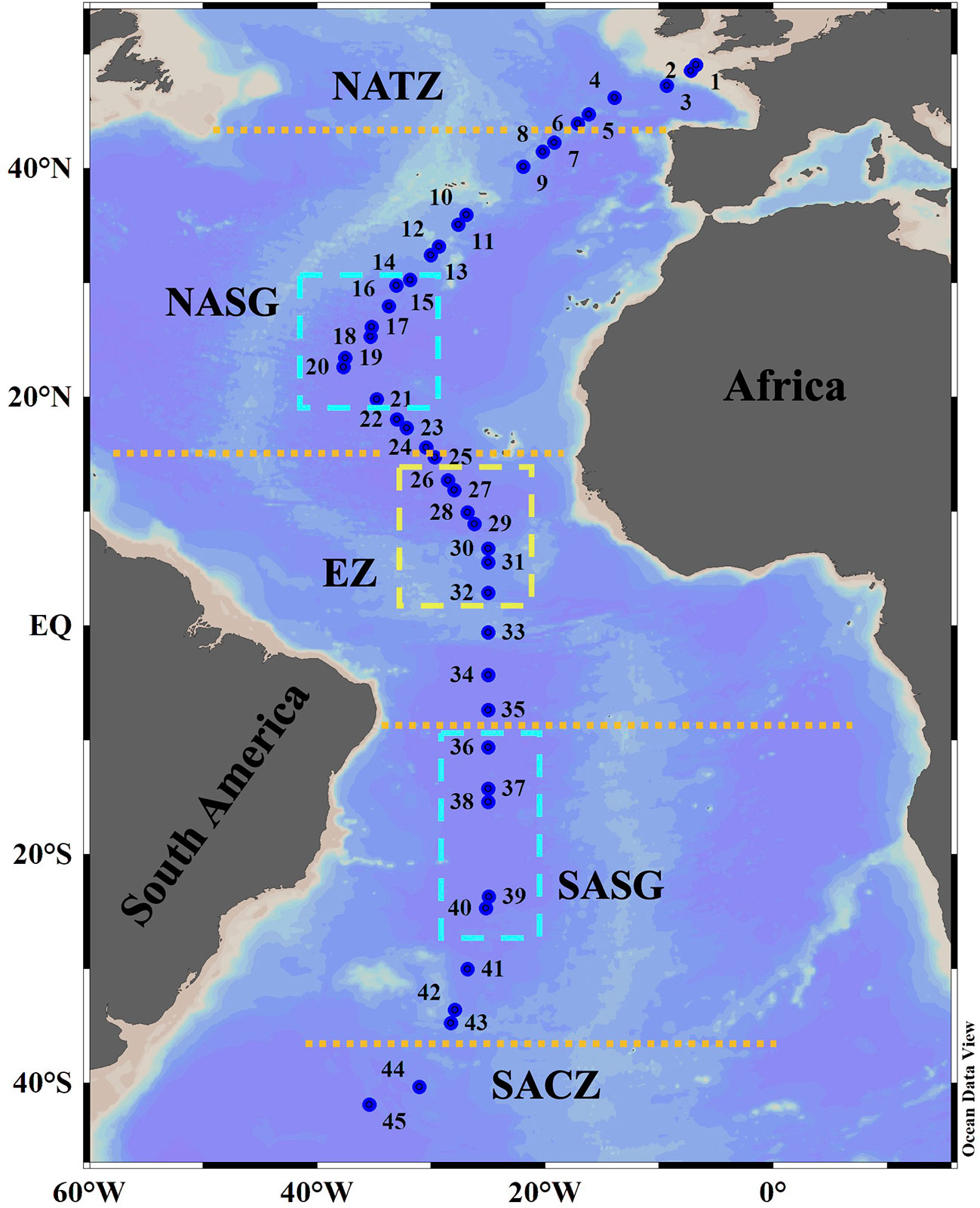
Figure 1 Location of sampling stations on the AMT29 cruise. The boundary positions (orange dotted lines) of the North Atlantic Transition Zone (NATZ), Northern Atlantic Subtropical Gyre (NASG), Equatorial Zone (EZ), Southern Atlantic Subtropical Gyre (SASG) and South Atlantic Convergence Zone (SACZ) were determined according to environmental factors as defined by Aiken et al. (2000), Hooker et al. (2000) and Aiken et al. (2017). The yellow box indicates the Equatorial Zone centre. The cyan boxes delimit gyre centres.

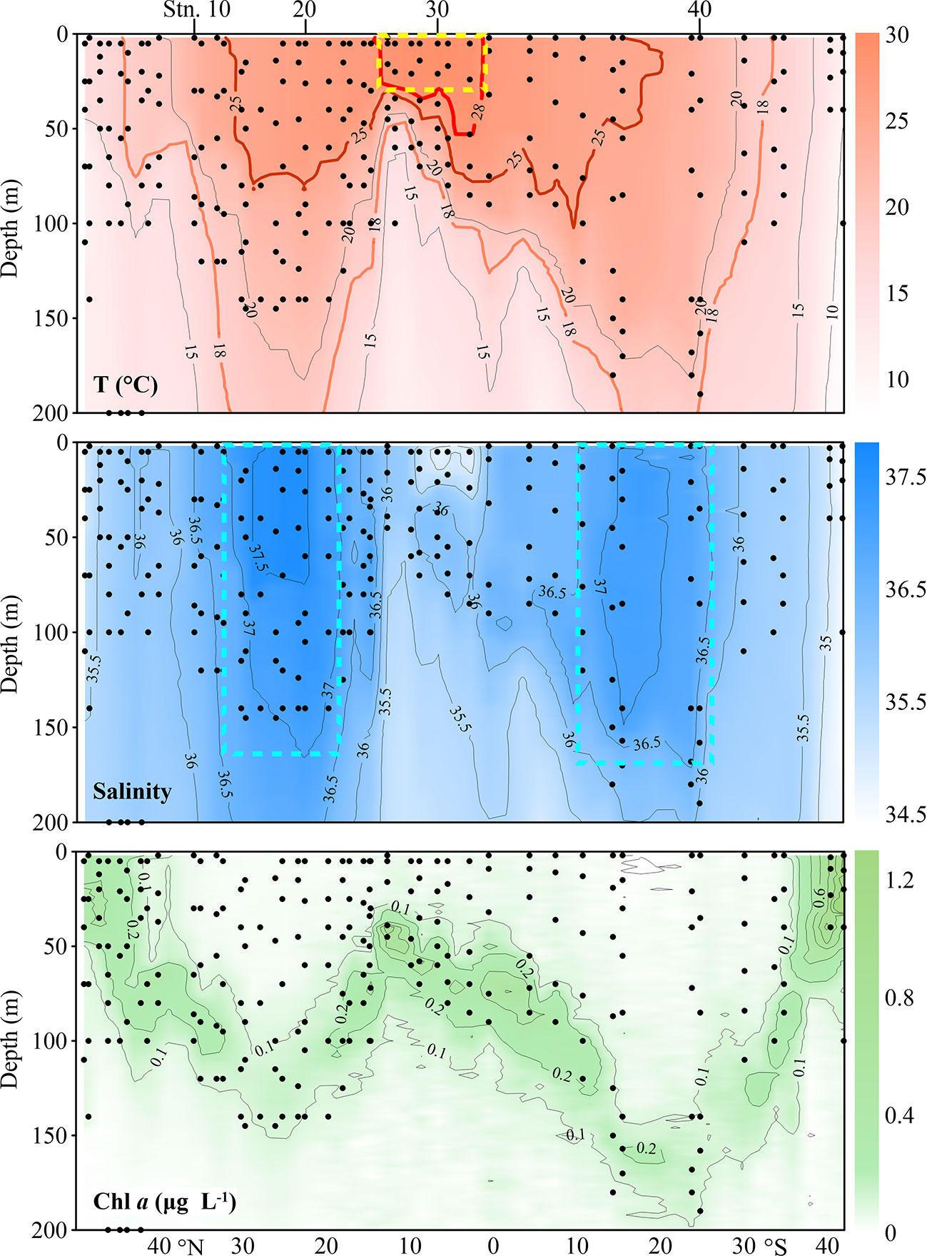
Figure 2 Distribution of temperature (T), salinity and in vivo chlorophyll fluorescence (Chl a) along the AMT transect. Each dot represents one sampling point. The yellow box indicates the Equatorial Zone centre. The cyan boxes delimit gyre centres. Black dots denote the locations of sample collection.

In the laboratory, each sample was settled in an Utermöhl counting chamber for at least 24 h and examined using an inverted microscope (Olympus IX 71, 100× or 400× magnification). As the Tintinnina protoplasts can easily detach from the lorica during sample collection and fixing (Paranjape and Gold, 1982; Alder, 1999; Gómez, 2007), empty Tintinnina loricae were counted as living cells in our study. For each species, at least 20 individuals (if possible) of each species were photographed and measured. Tintinnina was identified to the lowest possible taxonomic level (usually species level) based on lorica morphology and size according to the literature (Kofoid and Campbell, 1929; Hada, 1937; Hada, 1938; Kofoid and Campbell, 1939; Bakker and Phaff, 1976; Yoo et al., 1988; Zhang et al., 2012).

The maximum abundance of one species in all the samples was labelled as A_max. The dominance index (Y) was calculated using the equation:

where N_i was the total number of individuals of the species i, N was total individual number of all species, f_i was the occurrence frequency of species i (number of sampling points occurred/number of all sampling points). Species with Y > 0.02 were defined as dominant species (Li et al., 2018). Species richness of one station is the total number of the species appeared in all the samples collected at this station.

The poleward edge positions of both Northern Atlantic Subtropical Gyre (NASG) and Southern Atlantic Subtropical Gyre (SASG) were defined as the boundary of the 0.15 μg L^-1 surface chlorophyll isopleth (Aiken et al., 2017). The Equatorial Zone (EZ) was located between 15°N and 10°S as defined by Aiken et al. (2000). North of the NASG was the North Atlantic Transition Zone (NATZ), while south of the SASG was the South Atlantic Convergence Zone (SACZ) (Hooker et al., 2000).

Results

Hydrography and oceanic province identification

Temperature along the transect was in the range of 8.02-29.25°C in the upper 200 m (Figure 2). Water temperature was highest (28-29.25°C) in the upper 50 m between 1°N and 13°N and decreased poleward. We defined waters with temperature > 28°C as tropical waters. The prominent equatorial upwelling was observed north of the equator. Spatially, the isotherms showed obvious “W” distribution patterns along the transect (Figure 2). Taking the 18°C isotherm as an example, it appeared at about 50 m depth around 10°N and went to a depth of more than 200 m between 22-31°N and 15-24°S in the northern and southern hemispheres, respectively. The isotherm depth then became shallower poleward and reached the surface at about 43°N and 31°S, respectively. At about 5°S, the 15°C isotherm indicated a weak upwelling. The temperature changed very little vertically in the southernmost stations (Figure 2).

Salinity was in the range of 34.50-37.73. Horizontally, salinity was low at 0-12°N, it increased poleward and maintained high values in both subtropical gyres, then decreased. Vertically, the salinity varied very little with depth (Figure 2). NASG had higher salinity than SASG. The gyre centres were defined as salinity 37.5 (approximately the position of T > 25°C) in NASG and 37 in SASG, respectively. Correspondingly, waters with 15°C< T< 25°C was defined as frontal areas in both hemispheres.

Chl a concentration ranged from undetectable to 1.29 μg L^-1. The DCM layer was quite shallow in the northernmost and southernmost stations and deepened toward the equator. The DCM layer was deepest at about 24°S (170 m) and at about 26°N (132 m) (Figure 2). Consistently, the DCM was deepest in the gyre centres (Figure 2). All the stations along the transect were located in five oceanic provinces. The positions of the NASG and SASG were 15°N-43°N and 10°S-35°S, respectively (Figure 1).

Tintinnina distribution patterns

In total, 172 species were distinguished (five were unidentified species and 167 represented 40 genera) (Table 1). Protorhabdonella curta, Acanthostomella minutissima, Dadayiella ganymedes and Ascampbelliella armilla were the four most common species that occurred in 172, 170, 169 and 160 samples, respectively. There were 32, 30, 50, and 29 species occurring in more than 50 samples, 30-50 samples, 10-30 samples and 5-10 samples, respectively. The remaining 31 species were observed in fewer than 5 samples.

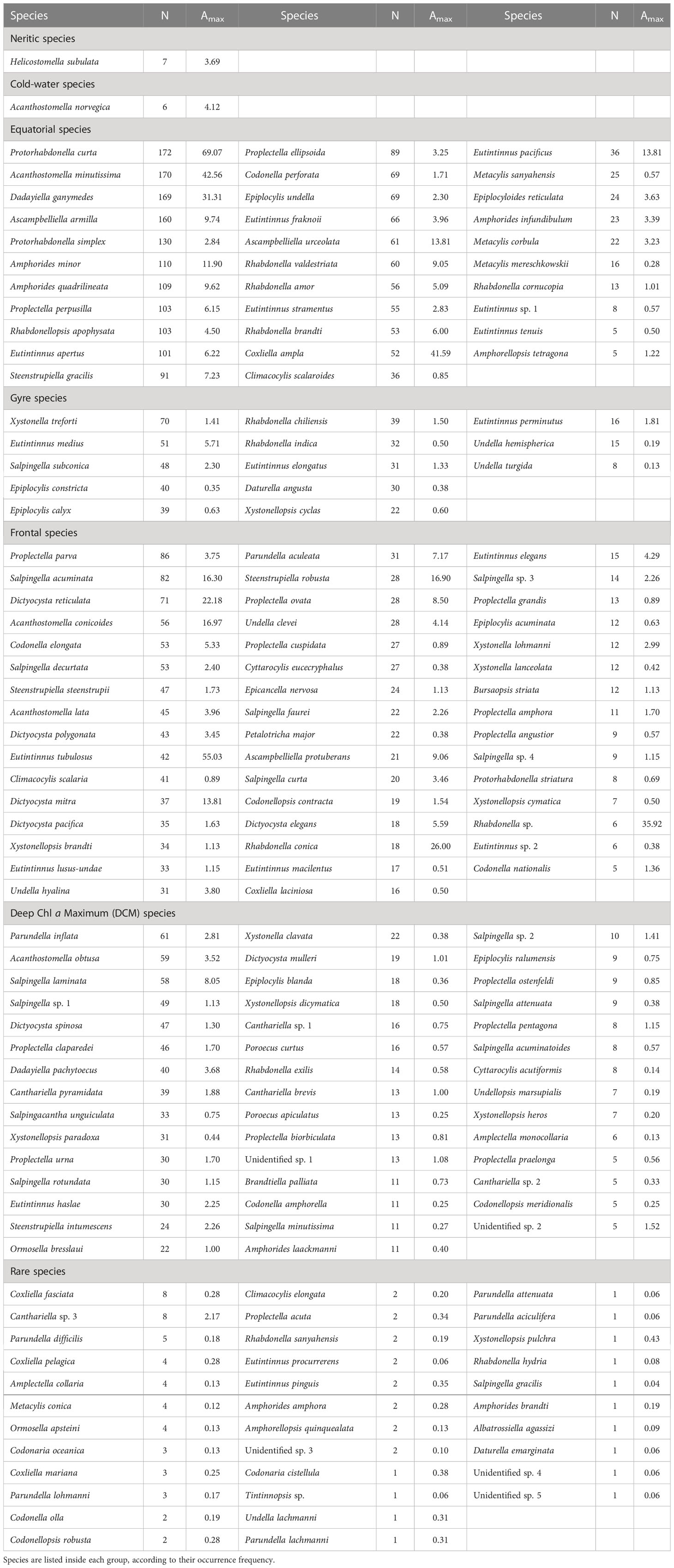
Table 1 Number of samples (N) where a given Tintinnina species was observed and maximum abundance (A_max, ind. L^-1) for each Tintinnina species along the Atlantic Meridional Transect.

A_max of Tintinnina species was positively related to their occurrence frequency (Supplementary Figure 1). Protorhabdonella curta, which had the highest occurrence frequency, had the highest A_max (69.07 ind. L^-1), at 40 m depth, St. 44 (Table 1). Only 15 Tintinnina species had A_max higher than 10.00 ind. L^-1. The A_max of most species (142 species) was lower than 5.00 ind. L^-1. There were 83 species with A_max lower than 1.00 ind. L^-1 (Table 1).

It was also difficult to define the biogeographic distribution patterns of the 31 species observed in< 5 samples because of their low occurrence frequency. Although Coxliella fasciata, Canthariella sp. 3 and Parundella difficilis occurred in ≥ 5 samples, their distributions were too scattered to determine their biogeographic distribution patterns. Thus, those 34 species were considered as rare species (Table 1). The largest A_max among rare species was 2.17 (ind. L^-1).

The neritic species Helicostomella subulata only occurred in the northernmost two stations, while the cold-water species Acanthostomella norvegica only appeared in the southernmost two stations (Figure 3; Supplementary Figure 2).

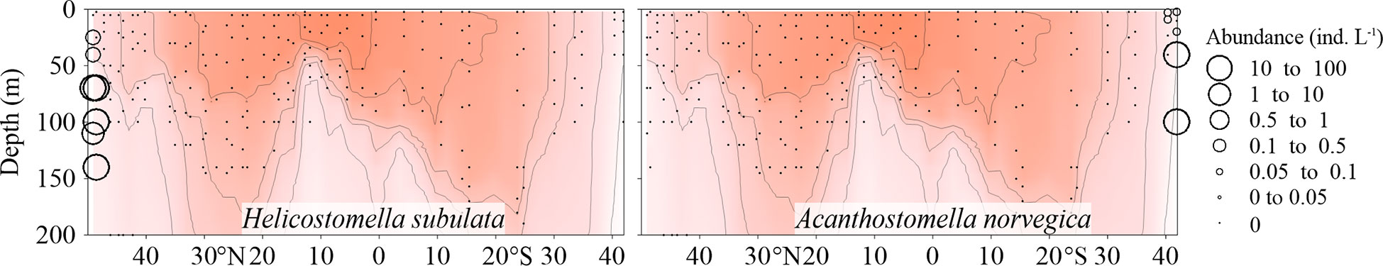
Figure 3 Vertical abundance (ind. L^-1) distribution of Helicostomella subulata and Acanthostomella norvegica along the AMT transect. The red color and isothermal lines are temperature (°C) as in Figure 2. Black dots denote the locations of sample collection.

All the other 136 species were warm water species. Based on their high abundance regions, they were classified into 4 biogeographic types: equatorial species, gyre species, frontal species (these three types had high abundance in the upper water< 75 m) and deep Chl a maximum species with high abundance in deeper water (> 75 m) (Figure 4; Supplementary Figures 3-10). Because some species showed slightly different distribution between the northern and southern hemispheres, their classification is based primarily on the distribution characteristics in the northern hemisphere.

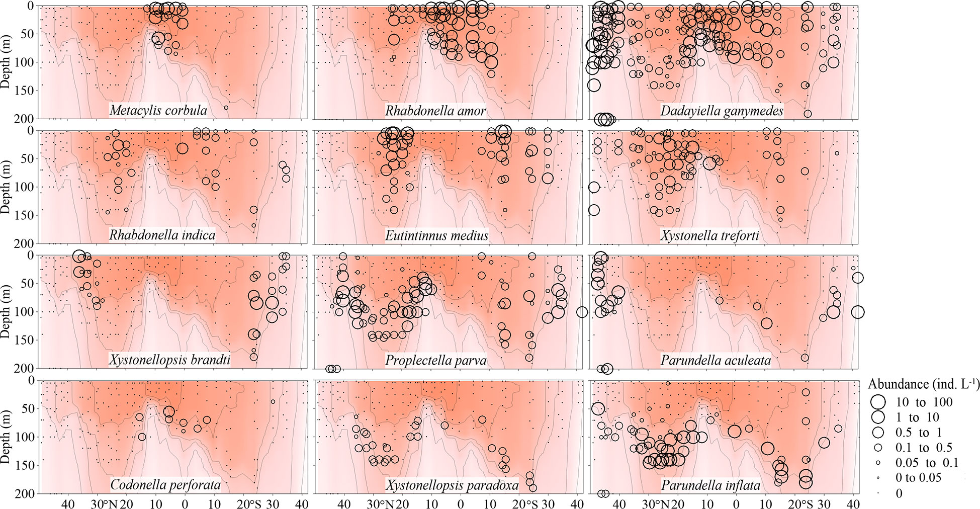
Figure 4 Vertical abundance (ind. L^-1) distribution of typical Tintinnina species in each biogeographic region along the AMT transect: from top to bottom, equatorial species, gyre species, frontal species and Deep Chl a Maximum species. The red color and isothermal lines are temperature (°C) as in Figure 2. Black dots denote the locations of sample collection.

A total of 32 species in 17 genera were considered as equatorial species (Figure 4; Supplementary Figures 3, 4 and Table 1) occurring in upper waters with temperature > 28°C. Among them, only some occurred in a narrow latitudinal range near the equator (such as Eutintinnus tenuis, Amphorellopsis tetragona, Amphorides infundibulum, Metacylis corbula and Coxliella ampla). These species were concentrated in the EZ with high surface temperature and also appeared in deep Chl a maximum waters with relatively low temperature. However, they were not detected in adjacent stations where the temperature was still high.

Some equatorial species had a high abundance in the equatorial region and their abundance decreased poleward (such as Eutintinnus stramentus, E. fraknoii, Protorhabdonella simplex and Steenstrupiella gracilis). Acanthostomella minutissima, Dadayiella ganymedes, P. curta had the widest temperature ranges. They were in high abundance not only in the EZ stations, but also in the northernmost and southernmost stations. These species had a wide temperature range and were noted over almost all the transect. Some equatorial species had very high A_max. For example, the A_max of four species (P. curta, A. minutissima, Coxliella ampla, D. ganymedes) were higher than 30 ind. L^-1.

A total of 13 Tintinnina species in 7 genera mainly observed in upper waters near the gyre centres and restricted to the NASG and SASG were defined as gyre species (Figure 4; Supplementary Figures 5, 6 and Table 1). They seldom occurred in waters with temperature outside the interval 18-28°C. Gyre species usually had low maximum abundance (A_max< 5.71 ind. L^-1).

A total of 47 species in 18 genera were frontal species and were mainly observed in upper waters of the gyres but not in the gyre centres themselves, being absent in waters with temperature > 28°C (Figure 4; Supplementary Figures 7, 8 and Table 1). Those species had high abundance in the frontal area where different water masses met and interacted, both horizontally and vertically. They formed a narrow band in the frontal area. For example, Xystonellopsis brandti occurred between 20-25°C in the northern hemisphere. Similarly, Proplectella parva occurred between 18-20°C and Parundella aculeata between 15-18°C (Figure 4). The largest A_max was 55.03 ind. L^-1 for Eutintinnus tubulosus. Eight species had A_max > 10 ind. L^-1. Some species (e.g., P. parva, Salpingella acuminata, Acanthostomella lata, A. conicoides) showed obvious tropical submergence phenomenon: occurring throughout the water in high latitude but in deeper layers of tropical waters where temperatures are lower than in the upper layers.

Deep Chl a maximum species included 44 species in 21 genera occurring in deep waters but disappeared in upper (< 75 m) warmer waters (Figure 4; Supplementary Figures 9, 10 and Table 1). All of the deep Chl a maximum species had A_max lower than 10 ind. L^-1.

Asymmetric geographic distribution in northern and southern hemispheres

Asymmetric distribution of Tintinnina species along the latitudinal gradient was a frequent phenomenon, especially in the NASG and SASG zones (Supplementary Figures 3, 5, 7, 9). Some species were restricted to only one hemisphere. Some frontal species (e.g., Codonella nationalis, Rhabdonella conica, Xystonella lohmanni, Steenstrupiella robusta and Proplectella ovata) only appeared in the northern hemisphere in this study, while Epiplocylis acuminata, Proplectella angustior, Proplectella amphora, Bursaopsis striata, Protorhabdonella striatura and Protorhabdonella sp. only occurred in the southern hemisphere (Supplementary Figure 7).

Some species showed different temperature range tolerance between the two hemispheres, such as Acanthostomella conicoides and Proplectella urna. Abundance of A. conicoides was high when the temperature was in the range of 15-18°C in the northern hemisphere, but almost disappeared in the same temperature range in the southern hemisphere (Supplementary Figure 7). P. urna exhibited high abundance when the temperature was about 25°C in the southern hemisphere, but its high abundance in the northern hemisphere appeared when the temperature was about 20°C (Supplementary Figure 9). Other examples were P. perpusilla, Amphorides quadrilineata (Supplementary Figure 3), Rhabdonella chiliensis (Supplementary Figure 5). Together with differences in the temperature range, the bandwidth of the vertical distributions of some frontal species (e.g., Xystonellopsis brandti, P. parva, Parundella aculeata) (Figure 4) was narrower in the northern hemisphere than in the southern hemisphere.

The vertical distribution of some species was likewise different in the two hemispheres. Proplectella claparedei and Acanthostomella obtusa occurred in surface waters in the southern hemisphere. In contrast, they were not observed in surface waters in the northern hemisphere (Supplementary Figure 9).

The relative locations of some species were dissimilar between the two hemispheres. For example, Eutintinnus perminutus, Epiplocylis calyx were on the poleward side of E. medius in the northern hemisphere, but vice versa in the southern hemisphere (Supplementary Figure 5).

Tintinnina species richness and abundance

Total abundance of equatorial species was highest in the EZ, decreased poleward and then increased at both boundaries of the transect, especially the northern one (Figure 5). The number of equatorial species at each sampling point decreased from the warm centre to both sides (Figure 6). The Gyre Species exhibited high values in the gyre centres regarding both abundance and number, with a declining trend toward the equator and poles (Figures 5, 6). The frontal species were present in high abundance and number in the AMT frontal areas (Figures 5, 6). In the DCM layer, the deep Chl a maximum species were also observed in high abundance (Figures 5, 6).

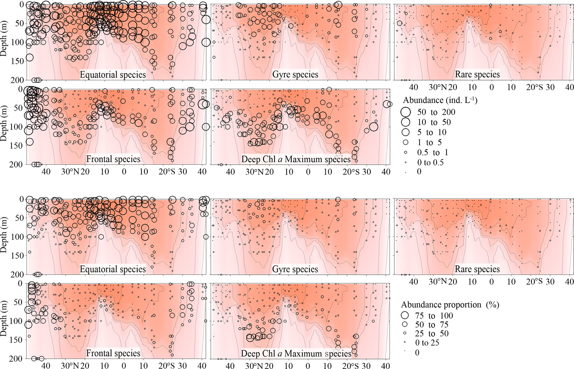
Figure 5 Vertical Tintinnina abundance (ind. L^-1, upper panel) and abundance proportion (%, lower panel) distribution in each biogeographic region along the AMT transect. The red color and isothermal lines are temperature (°C) as in Figure 2. Black dots denote the locations of sample collection.

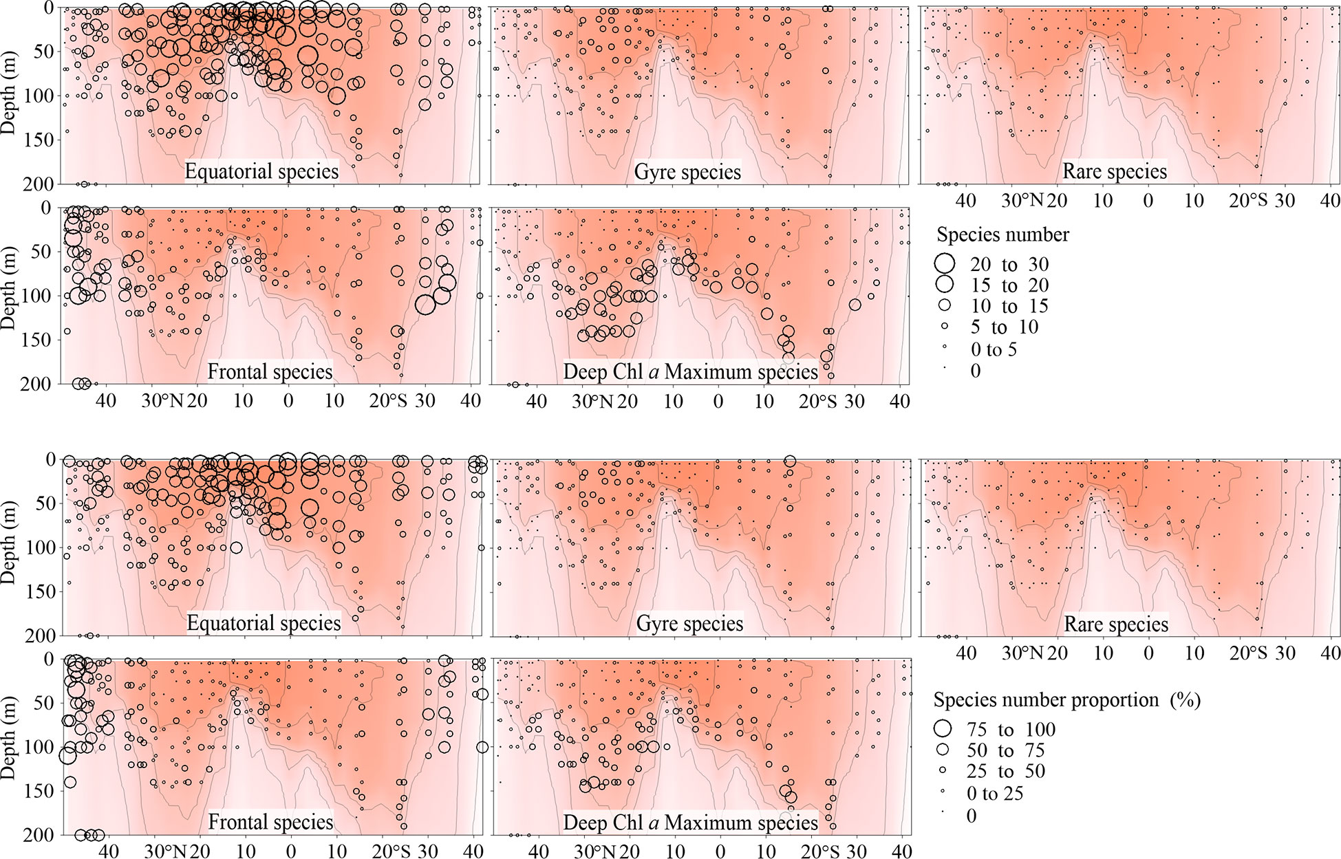
Figure 6 Vertical distribution of Tintinnina species number (upper panel) and proportion (%, lower panel) in each biogeographic region along the AMT transect. The red color and isothermal lines are temperature (°C) as in Figure 2. Black dots denote the locations of sample collection.

Tintinnina species richness was in the range of 3-45, with elevated values mainly belonging to the 50-150 m layer between 40°N and 35°S, at most stations. The highest value (45) was determined for the 110 m sample of Stn. 41. In the upper 50 m, Tintinnina species richness was relatively low (Figure 7).

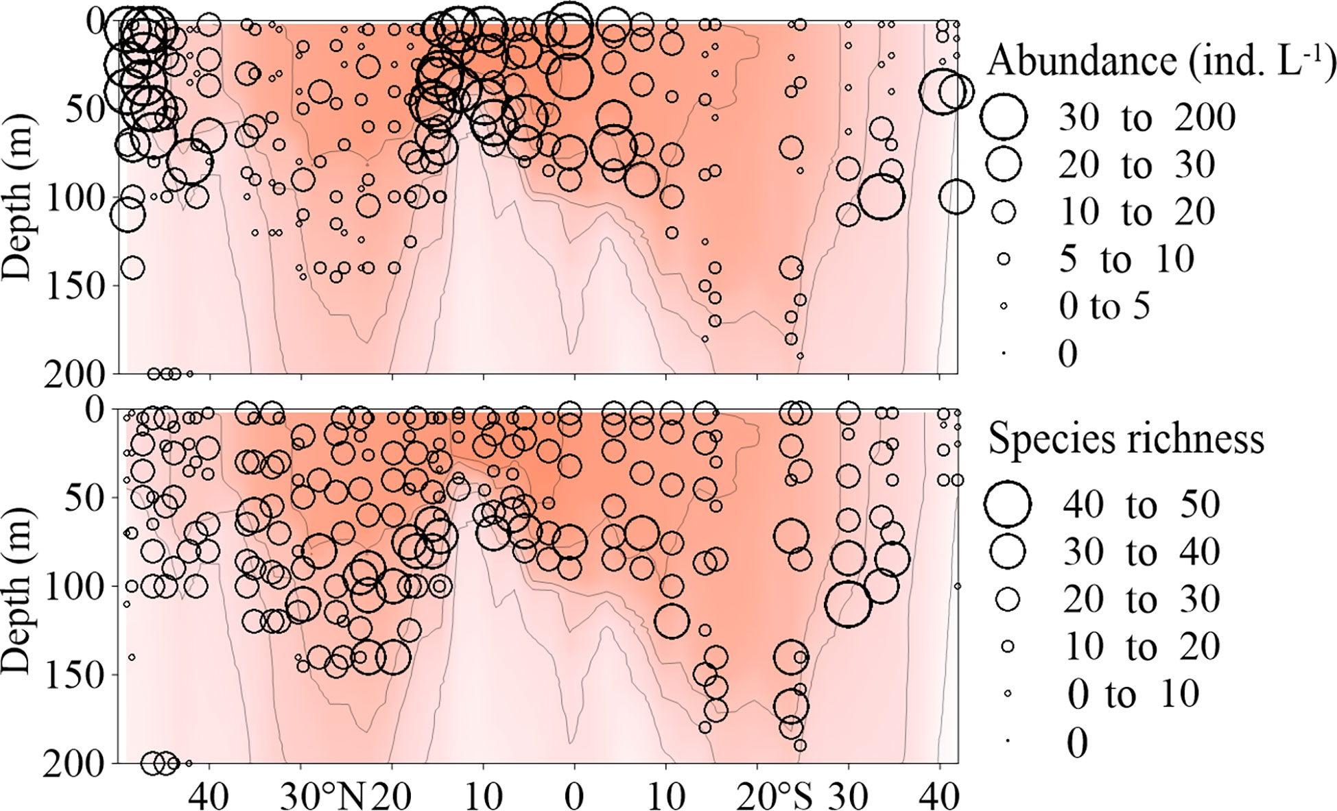
Figure 7 Vertical distribution of Tintinnina abundance (ind. L^-1) and species richness along the AMT transect. The red color and isothermal lines are temperature (°C) as in Figure 2. Black dots denote the locations of sample collection.

Tintinnina abundance varied between 0.33 and 185.11 ind. L^-1, and was characterized by a distribution pattern completely different from that of their species richness. Tintinnina abundance was< 50 ind. L^-1 in most samples, high values mainly belonged to the upper 100 m in the northernmost and southernmost stations, as well as regions around the equator. Tintinnina abundance was extremely low in the centres of both NASG and SASG (Figure 7).

Tintinnina species richness increased with temperature, reaching peak value at about 20°C, then decreased slightly when the temperature exceeded 20°C. In contrast, Tintinnina abundance did not vary much with temperature. Species richness increased with salinity and peaked at a salinity of about 36.5. On the other hand, Tintinnina abundance decreased when salinity increased. Tintinnina species richness and abundance increased when Chl a was lower than 0.4 μg L^-1, and decreased sharply when the Chl a exceeded 0.4 μg L^-1 (Figure 8).

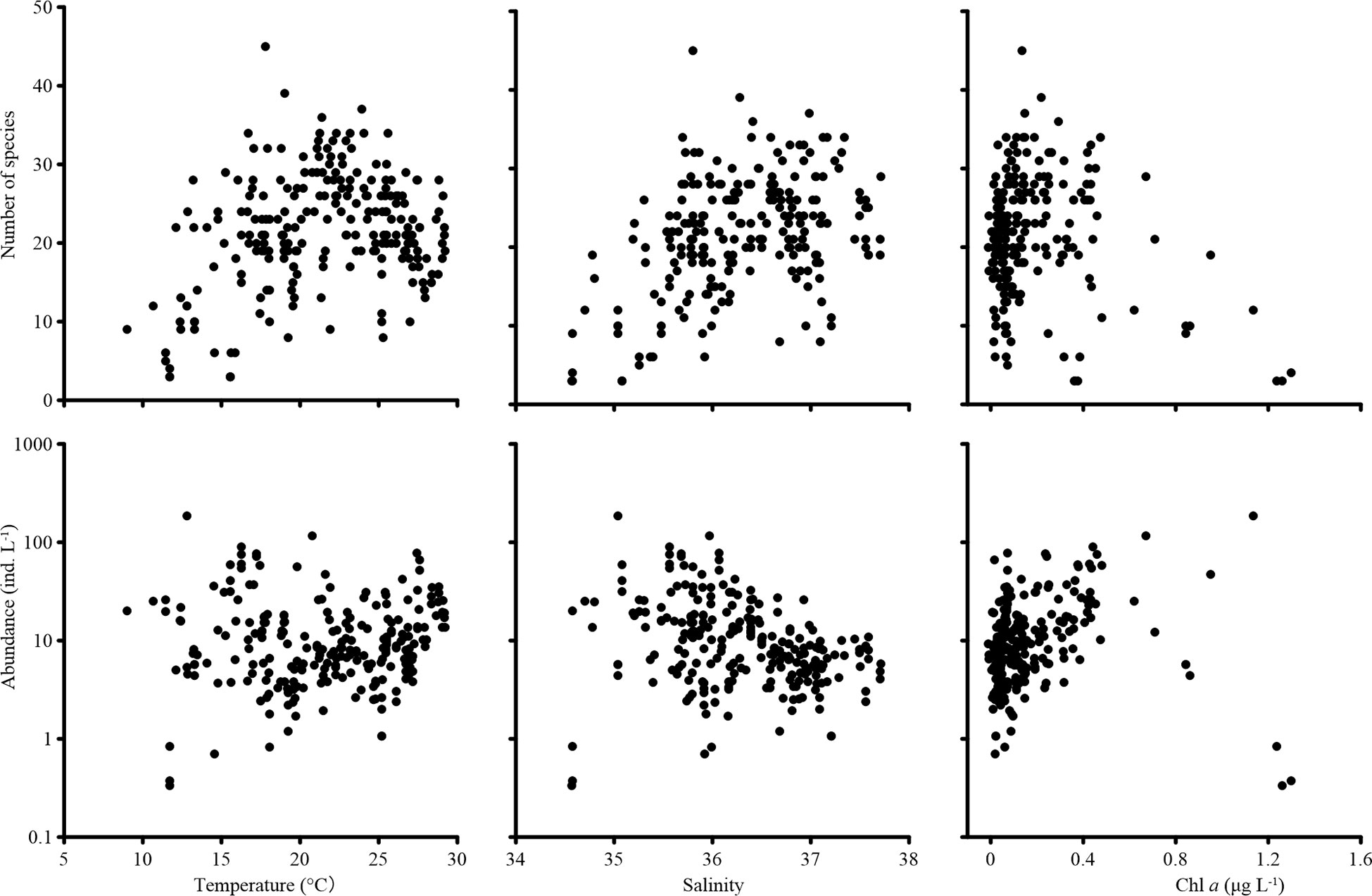
Figure 8 Tintinnina species richness and abundance variation with temperature, salinity, and in vivo chlorophyll a fluorescence (Chl a).

Organization of Tintinnina assemblage by sub-assemblages

Since all the species were mainly classified into 4 biogeographic types, all the species in a particular biogeographic type could be considered as a sub-assemblage. Therefore, the Tintinnina assemblage could be deemed as the superposition of four sub-assemblages: equatorial, gyre, frontal and deep Chl a maximum sub-assemblages. The dominance of each sub-assemblage in the different parts of the transect was evaluated by means of the abundance percentage and species number percentage of each sub-assemblage in the Tintinnina assemblage (Figures 5, 6). Deep Chl a maximum sub-assemblage was the dominant assemblage in waters below 100 m depth because it occupied > 50% in both Tintinnina abundance and species number.

In the waters shallower than 100 m, equatorial sub-assemblage abundance occupied >50% of total Tintinnina abundance in most stations. Its species number occupied >50% of total Tintinnina species number in equatorial and gyre zones and decreased in frontal zones. Therefore, equatorial sub-assemblage dominated the equatorial and gyre zone upper 100 m waters. Frontal sub-assemblage abundance and species number were >50% of respectively Tintinnina abundance and species number in the frontal zone upper waters. Since equatorial species also showed values >50% in this area, we concluded that the frontal and equatorial sub-assemblages co-dominated in the frontal zones. Gyre sub-assemblage distributed in the upper waters of the gyres. Their abundance exceeded 50% in only two samples and their species number exceeded 50% in only one sample. Therefore, gyre sub-assemblage seldom dominated in the transect.

To further compare the influence of the sub-assemblages in the equatorial centre and gyre centres, the dominant species and their abundance contribution to total Tintinnina abundance was estimated (Table 2). In equatorial centre, all of the dominant species were equatorial species. In the gyre centres, the gyre species Eutintinnus medius was the first dominant species in the NASG and SASG centres. The frontal species Rhabdonella brandt and Proplectella cuspidata were dominant in the NASG and SASG centres, respectively.

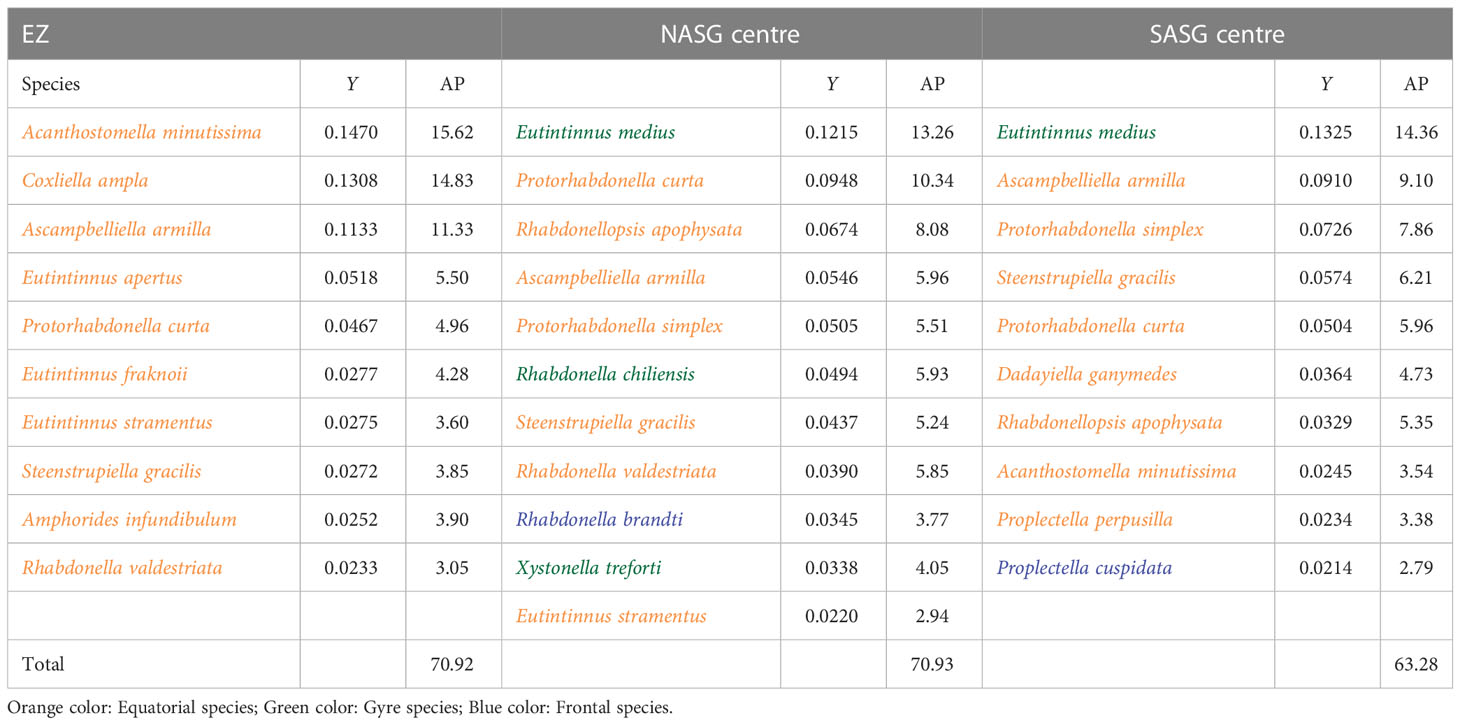
Table 2 Dominance index (Y) and abundance proportion (AP, %) of each dominant species in the upper 40 m of the Equatorial Zone (EZ), Northern Atlantic Subtropical Gyre (NASG) centre and Southern Atlantic Subtropical Gyre (SASG) centre shown in Figure 1.

Tintinnina assemblage in different zones along the transect

The transect completely crossed the NASG, EZ and SASG, enabling us to reliably describe the Tintinnina assemblage structures in these regions. The number of Tintinnina species in each biogeographic region was highest in the NASG (142 species), followed by the SASG (124 species), EZ (110) and NATZ (75). Only 23 species were recorded in the SACZ. In total, 14 Tintinnina species occurred in all 5 regions, and 37, 53 and 29 species appeared in 4, 3 and 2 regions, respectively. Numbers of species which were specific in the NATZ, NASG, EZ, SASG and SACZ were 6, 14, 8, 8 and 3, respectively. The NASG and SASG assemblages shared 111 Tintinnina species. Thirty-one species that occurred in the NASG were not observed in the SASG, while 13 species occurring in the SASG were absent in the NASG (Figure 9).

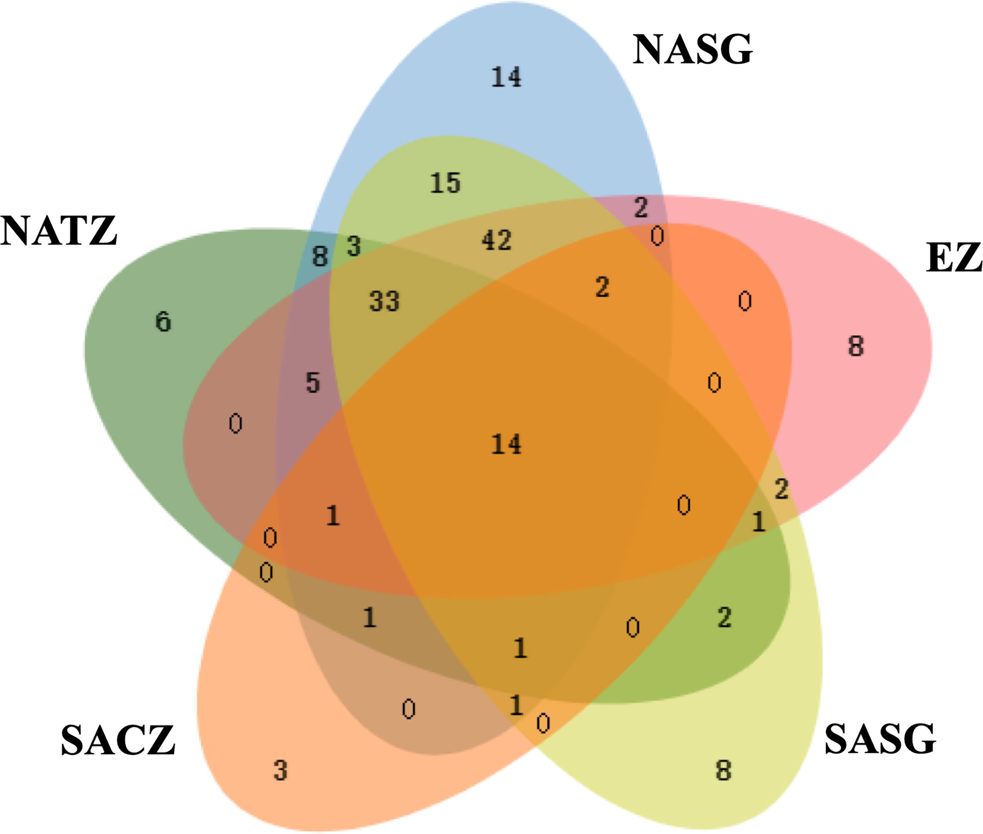
Figure 9 Venn diagram showing the number of Tintinnina species that are unique and shared among the five oceanic provinces. NATZ, North Atlantic Transition Zone; NASG, Northern Atlantic Subtropical Gyre; EZ, Equatorial Zone; SASG, Southern Atlantic Subtropical Gyre; SACZ, South Atlantic Convergence Zone.

There were 8, 4, 7, 7 and 6 dominant species in the NATZ, NASG, EZ, SASG and SACZ, respectively. Eutintinnus tubulosus and Dadayiella ganymedes were the top 2 dominant species in the NATZ with dominance index > 0.1. The dominance index of all the dominant species was< 0.1 in the NASG and SASG. In the EZ, Acanthostomella minutissima was the most dominant, while Coxliella ampla was the second most dominant species, with dominance index of 0.18 and 0.11, respectively. Finally, A. minutissima, Protorhabdonella curta, D. ganymedes and A. armilla were the dominant species in all the samples along the transect (Table 3).

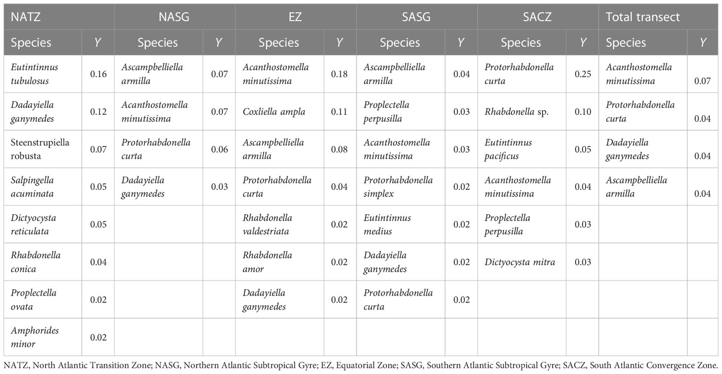
Table 3 Dominant species and their dominance index (Y) in each biogeographic region and the total transect.

The dominant species composition varied with different biogeographic regions. Most dominant species in the NATZ disappeared or had extremely low dominance indexes in other regions except for Dadayiella ganymedes, which was also dominant in the NASG, EZ and SASG and it was not observed in the SACZ. Eutintinnus tubulosus was the first dominant species in the NATZ, but its dominance index was extremely low in NASG and EZ and could not be determined in SASG and SACZ. Rhabdonella conica was the dominant species in the NATZ but was absent in the other four regions (Table 3).

The 4 dominant species in the NASG were also dominant in the EZ and SASG. Acanthostomella minutissima and Protorhabdonella curta were dominant in the NASG, EZ, SASG and SAC; their dominance index was< 0.005 in the NATZ. Ascampbelliella armilla was the dominant species in the NASG, EZ and SASG, but its dominance index was very low in the NATZ and did not appear in the SACZ. The EZ, SASG and SAC contained 3, 3 and 4 specific dominant species, respectively (Table 3).

Latitudinal species richness gradient of Tintinnina

Latitudinally, Tintinnina species richness ranged from 6 to 71 (Figure 10) and showed an asymmetric bimodality with a dip near the equator. The northernmost and southernmost stations in both hemispheres, Stn. 1 at about 49°N and Stn. 45 at about 42°S, had the lowest species richness. The Tintinnina species richness increased towards the equator, peaking at Stns. 18 and 20 (about 20°N), and Stns. 39 and 41 (23°S and 30°S), respectively (Figure 10).

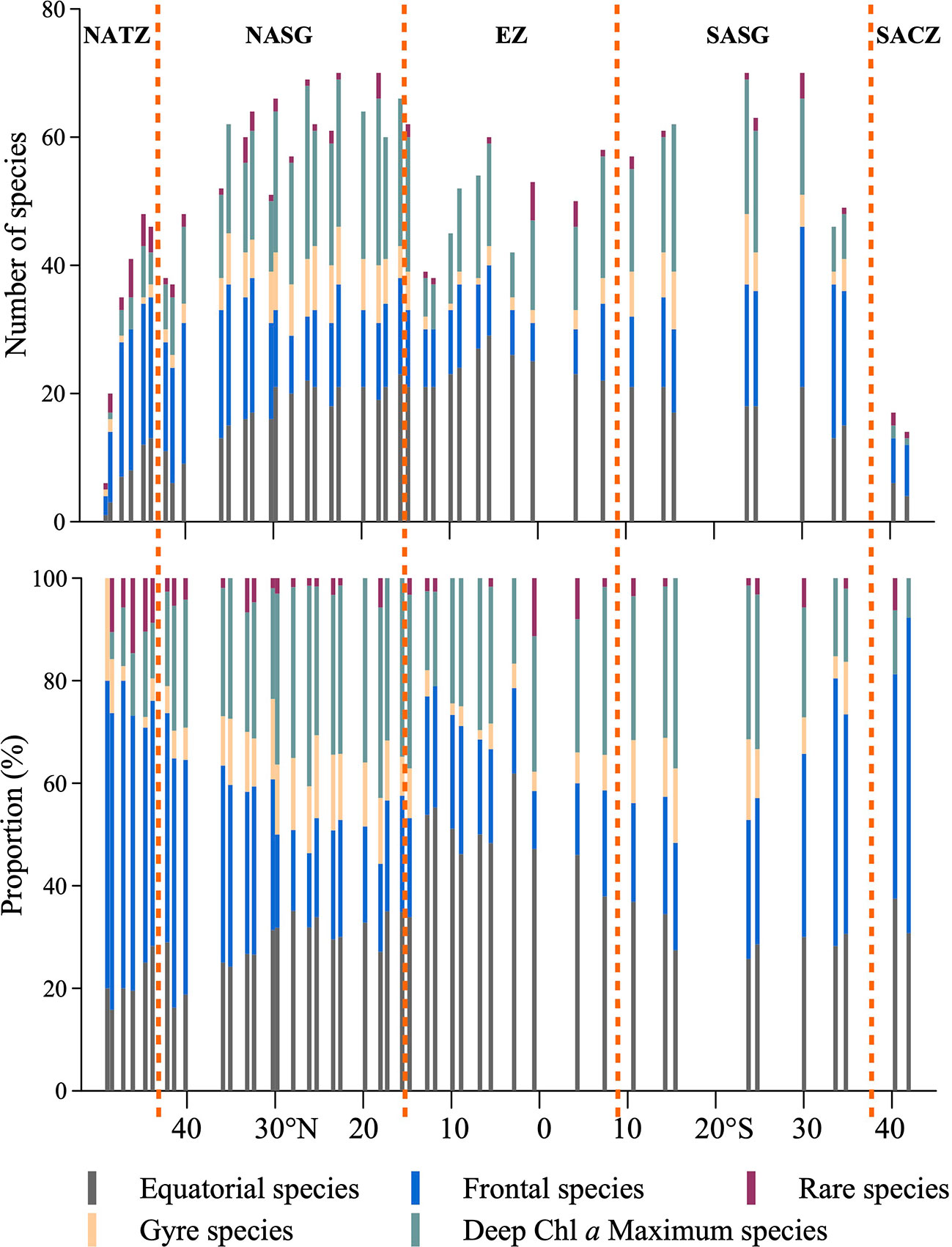
Figure 10 Latitudinal variation of Tintinnina species-number in each biogeographic pattern along the AMT transect. NATZ, North Atlantic Transition Zone; NASG, Northern Atlantic Subtropical Gyre; EZ, Equatorial Zone; SASG, Southern Atlantic Subtropical Gyre; SACZ, South Atlantic Convergence Zone.

Along the transect, the number of equatorial species showed a unimodal peak in the equatorial zone. Frontal species had a high species number at both ends of the transect. Gyre species and deep Chl a maximum species showed bimodal peaks at the gyre centres. The total number of Tintinnina species, i.e., the superposition of the four types and rare species, showed bimodal peaks at the gyre centres (Figure 10).

Discussion

Biogeography of Tintinnina species

Previous knowledge of the geographic distribution of most Tintinnina species is largely incomplete, especially in regions of intricate and costly accessibility (Menegotto and Rangel, 2018). Dolan et al. (2013) and Pierce and Turner (1993) classified Tintinnina into 5 biogeographic distribution patterns at the genus level. Although some genera were considered as cosmopolitan, there appears to be no species that is truly cosmopolitan (Dolan et al., 2013). However, information on Tintinnina biogeographic distribution at the species level was scarce (Dolan et al., 2013; Li et al., 2019; Li et al., 2021). Tintinnina abundance was extremely low in tropical and subtropical open waters (Dolan et al., 2007; Gómez, 2007; Zhang et al., 2017; Li et al., 2018). In this study, we found that the maximum abundance of 83 Tintinnina species were lower than 1 ind. L^-1. Thus, sampling only 1 litre of water sample may miss many Tintinnina species with low abundance. It is worth noting that, in this study, the same person identified the Tintinnina species in all the collected samples and counted under the same protocol to minimize any potential human impact. Therefore, the method in this study could highlight the distribution pattern of most Tintinnina species except the rare ones. To our knowledge, this is the first species-level study on Tintinnina distribution and assemblage composition in the Atlantic Ocean.

In order to explore the biogeographic distribution patterns of Tintinnina in warm waters, we collected samples across a large spatial span from about 50°N to 40°S. Helicostomella subulata was a neritic species and commonly reported in coastal waters of the Arctic and subarctic regions (Dolan et al., 2021; Li et al., 2021). Acanthostomella norvegica was usually found in high-latitude waters of both hemispheres (Li et al., 2016; Liang et al., 2020; Li et al., 2021). The occurrence of H. subulata in the two northernmost stations and A. norvegica in the two southernmost stations, indicated that the sampled transect crossed the full span of both NASG and SASG. Thus, the data in this study allowed us to analyse the Tintinnina biogeographic distribution over a large span of warm waters.

Most species identified in our study belonged to warm-water and cosmopolitan genera according to Dolan et al. (2013). Metacylis was considered as a neritic genus by Dolan et al. (2013). Li et al. (2016) classified Metacylis as a cosmopolitan genus. In the present study, four species of the genus Metacylis were recorded. None of them occurred in the northernmost two coastal stations. Metacylis sanyahensis, M. corbula and M. mereschkowskii were considered as equatorial species. M. conica was a rare species occurring in only 4 out of 235 samples in our study.

Li et al. (2021) investigated surface Tintinnina assemblage variation along transects across the North Pacific Transition Zone in summertime. They grouped 41 Tintinnina species into boreal, warm water type I, warm water type II, transition zone and cosmopolitan groups, according to the region where they were recorded and their abundance distribution patterns along the temperature gradient. Dadayiella ganymedes and Eutintinnus tubulosus were classified as warm water type I species, their abundance was high at the transition zone and decreased towards the equator (Li et al., 2021). In the East China Sea, high abundance of D. ganymedes appeared in the frontal area generated by the interaction between the Kuroshio current and coastal waters (Li et al., 2016). Those studies were based on the surface Tintinnina distribution. In the present study, the surface abundances of D. ganymedes and E. tubulosus were extremely high in the northern boundary of NASG, decreased towards the equator and had a slight increase in the EZ. However, D. ganymedes and E. tubulosus had high abundance at the subsurface waters in the EZ. Thus, we classified D. ganymedes and E. tubulosus as equatorial species.

Vertically, the present study showed that some species had surface abundance peaks, whereas others exhibited abundance peaks at the DCM layer. These characteristics are consistent with Tintinnina in the tropical Pacific Ocean (Wang et al., 2019). Phytoplankton species were likewise classified into shallow (upper 30 m) and deep (DCM) groups in the Pacific Ocean, which offered suitable food supplies for ciliates to prey on (Venrick, 1988). Our research only sampled waters above the DCM, except at some stations in the north end of the transect. Tintinnina abundance decreased sharply below the DCM in the tropical Pacific waters (Li et al., 2018). Therefore, it is likely that the Tintinnina abundance in the AMT transect peaks at the DCM and decreases sharply below DCM.

Tropical submergence of transition zone species

Some equatorial and gyre species showed wide temperature tolerance, horizontally and vertically. They appeared in deeper colder waters but did not expand poleward. In contrast, tropical submergence was common for frontal species whose distribution coincided with the isotherm downward trend, occurring in high-latitude surface waters and detected in deep waters of the equatorial zone. Tropical submergence (Chaudhary et al., 2021) plays a significant role in the composition of low and mid-latitude plankton assemblages. Some species present near the surface at mid-high latitudes are well known to follow isothermal pathways into intermediate and abyssal water depths at low latitudes (Trubovitz et al., 2020). To our knowledge, it is the first time that Tintinnina tropical submergence is reported.

More and more researchers have realised the importance of investigating the vertical distribution of plankton species, like in the central Atlantic Ocean where four mesozooplankton groups were vertically distinguished (Vedenin et al., 2022). Preliminary studies have also shown that Tintinnina can be vertically distributed according to different groups (Wang et al., 2020; Wang et al., 2021). The fact that Tintinnina species observed in high latitude surface waters can be detected in low latitude deep waters forces one to consider the roles of both depth and latitude when investigating Tintinnina biogeographic distribution patterns.

Thanks to the large latitudinal coverage and vertical sampling, we found a lot of frontal Tintinnina species, which occurred in narrow bands between subtropical gyre centre and subarctic gyre. Some plankton species found in the transitional zone between subarctic and subtropical gyres are called transitional zone species. Our study showed that frontal zone species had wider temperature range (approx. 15-25°C) than transitional zone (15-20°C) (Li et al., 2021). Undella clevei and U. californiensis were considered as transition zone species, mainly observed in the North Pacific Transition Zone in the 15-20°C temperature range (Li et al., 2021). This Tintinnina biogeographic characterisation was only based on surface data. In the present study, U. clevei showed an asymmetric distribution pattern between both hemispheres and was linked to the frontal systems of different water masses. In the southern hemisphere, the U. clevei distribution was associated with the 15-20°C isotherms. In the northern hemisphere, it was mainly present in NASG deep waters in the temperature range 20-25°C. This is the reason why U. clevei was identified as a frontal species in the present study. Although U. californiensis was not detected in our study, it was observed in the open Pacific Ocean (Gómez, 2007). We speculate that U. californiensis may also be subject to a tropical submergence phenomenon and might occur in waters deeper than the DCM layer in low latitudes.

Transition zone species were reported in some phytoplankton (Venrick, 1971) and macrozooplankton (Brinton, 1962; McGowan, 1971). However, the mechanism responsible for their presence in the eastward flow had no obvious explanation. Olson (2001) proposed that mesoscale eddies would transport some organisms counter current. Boltovskoy (1998) and Longhurst (2007) did not agree with this mechanism. Our data suggest that tropical submergence might be the mechanism accounting for the existence of transition zone species. Circular current is the base of plankton distribution (Longhurst, 2007). Some individuals submerged to the bottom of the gyre could survive the full cycle of the gyre flow and serve as seeds when they are released to the colder area, where vertical mixing brings them back to the upper water. However, these submerged individuals had low abundance and were neglected in biogeography studies. As a result, such species might in fact be frontal species but have been mistakenly regarded as transition zone species.

Conceptual model of organization of planktonic Tintinnina assemblage

According to the plankton biogeography theory of circular current distribution (Longhurst, 2007), except for the frontal sub-assemblage, the other three sub-assemblages could be divided into core areas with high abundance and species number, and pioneer areas as per Li et al. (2016). Species confined to the core area were called core species. Correspondingly, the species that had expanded out of the core area were referred to as pioneer species. Species belonging to the deep Chl a maximum sub-assemblage core area were found in the gyre deep waters, whereas pioneer species expanded out to the edge of the gyres. Some pioneer species could be brought into shallow waters by vertical mixing on the polar side of the gyre.

The core area of the gyre sub-assemblage was in the upper water around the gyre centre. Pioneer species expanded to both the warm and cold sides of the gyre, but they could not exist in waters warmer than 28°C and colder than 20°C (except Xysttonella treforti).

In the equatorial sub-assemblage, the distribution of the species was kept in the equatorial zone by the tropical gyre which is composed of equatorial current and equatorial counter current. Core species (Amphorides infundibulum, Metacylis corbula) were in waters warmer than 28°C. Some species have been recorded poleward as pioneer species due to their large suitable temperature range. Some of them were entrained poleward by the mixing between tropical gyre and subtropical gyre. Some species (e.g., Steenstrupiella gracilis, Rhabdonella brandti) died out when they are moved into cold waters.

Some equatorial species (e.g., Dadayiella ganymedes, Protorhabdonella curta) were strong enough to exist and flourish at the edge of the subtropical gyre. These species are so special that they could also be considered frontal species which could flourish in equatorial waters. But we artificially classify them as equatorial species.

The organization of the Tintinnina assemblage resulted from the superposition of the four sub-assemblages as in the conceptual model of Figure 11. Although different biogeographical patterns were identified in previous studies, the influence of the species of a particular biogeographical pattern was not evaluated (Longhurst, 2007). Since our study is the first of its kind, we could not compare Tintinnina with other plankton. However, we speculate that the single-celled protist plankton might have similar organization mechanism because of their lack of life history.

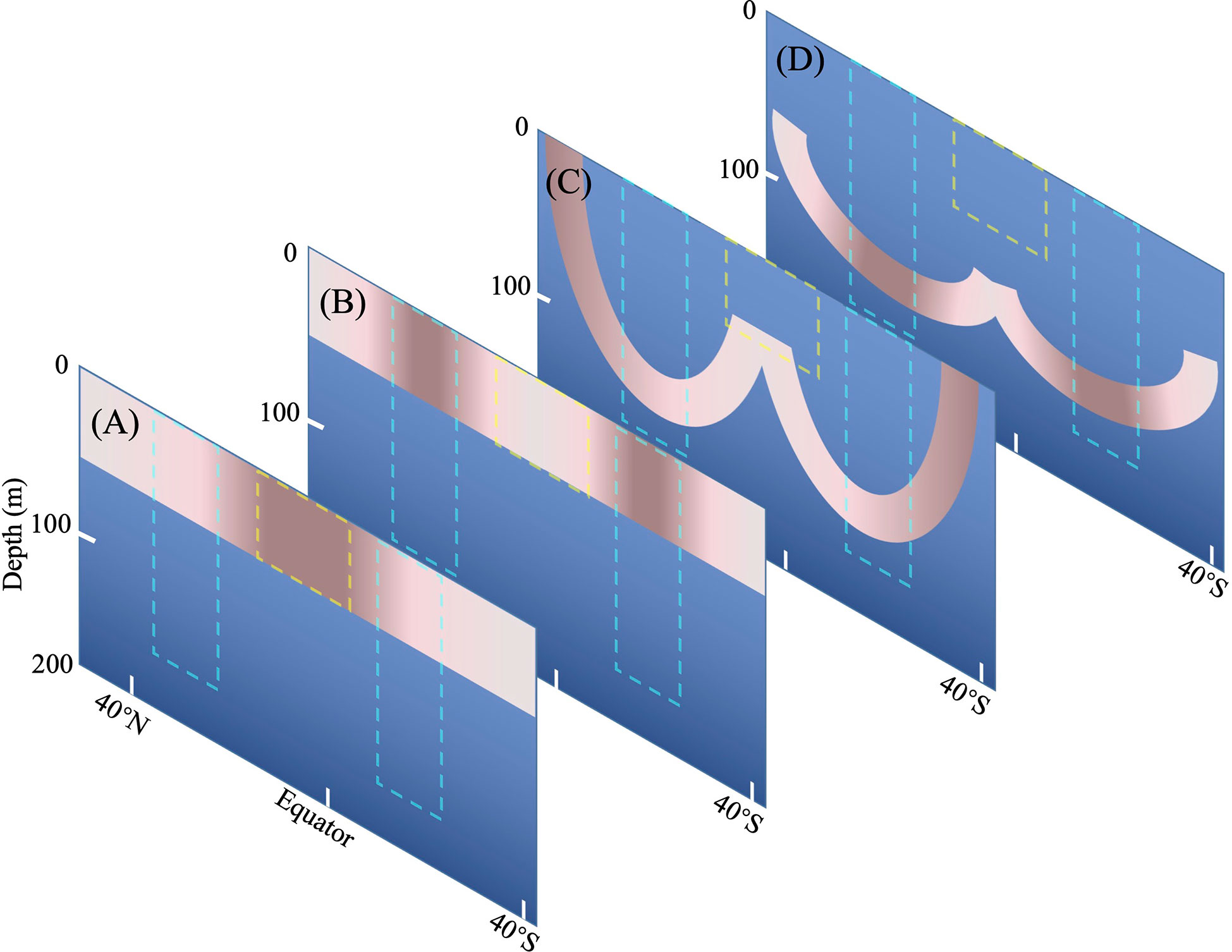
Figure 11 Conceptual model of Tintinnina communities composed of four sub-communities. (A) Equatorial sub-community, (B) Gyre sub-community, (C) Frontal sub-community, (D) Deep Chl a Maximum sub-community. The yellow box indicates the Equatorial Zone centre. The cyan boxes delimit gyre centres. Coral and rose color indicate the core and pioneer areas, respectively: the darker the color, the higher abundance and species richness.

Woods (1999) proposed a question: what is the change of plankton assemblage in a water-mass moving around the centre of north Atlantic Subtropical Gyre. Water-mass traveling from the Azores to the Antilles could take six years. It will take about five years to finish Sargasso-Sea circuit (Supplementary Figure 11). Our conceptual model suggests that, when a water-mass moves southward from Azores, individuals of frontal species in the upper water will gradually die out but some individuals in the deep water will remain alive to serve as seeds for the surface population. Some equatorial species will slowly get into the water-mass as it warms up. When the water-mass moves northward from Antilles, the seeds of frontal species might be mixed upward to upper water column and flourish again.

Differences of Tintinnina assemblages in NASG and SASG

Understanding the differences and similarities between the northern and southern hemispheres is necessary to monitor the changes that are occurring and are expected in the coming decades (Timmermann et al., 2015; Rodriguez et al., 2022). In the present study, Tintinnina diversity in both NASG and SASG was very high, encompassing 142 and 124 Tintinnina species, respectively. Both gyres shared 111 species which indicated a high similarity of the Tintinnina assemblage compositions in them.

Despite of the similarity of the Tintinnina compositions, 44 species were present in one gyre but not in the other. This non-symmetrical situation was also reported for Bacteria distribution by Sul et al. (2013), who observed fewer bacteria taxa in both hemispheres but more taxa than expected were only present in a single hemisphere. The Atlantic equatorial upwelling region (with a narrow vertical temperature range between 15°C to 25°C) has been identified as a strong ecological barrier for zooplankton dispersal, such as Copepoda (Goetze et al., 2017; Mcginty et al., 2021) and Mollusca Pteropoda (Burridge et al., 2015; Choo et al., 2021). Meanwhile, oceanic barriers are species-specific (Mcginty et al., 2021). As Tintinnina mobility is much weaker than that of mesozooplankton, it was not surprising that some Tintinnina species were separated by the EZ in the Atlantic Ocean. This may also be a universal phenomenon in warm waters of the open Pacific and Indian Oceans but need more investigations to be established.

The 111 shared species also showed different distribution patterns in NASG and SASG. Tintinnina distribution has been demonstrated to have notable seasonal differences (Camacho et al., 2015; Li et al., 2016; Rekik et al., 2020). This may be linked to the fact that some species have distinct temperature ranges in the two hemispheres.

The AMT transect crossed different part of the two subtropical gyres: through the middle of SASG but through the east side of NASG. This difference in transect relative position with the gyre centre might be the reason why some frontal species occupied narrower bands in the northern hemisphere than in the south. The weak upwelling at about 5°S might account for the relative difference in position between Eutintinnus perminutus, Rhabdonella indica and E. medius in the two hemispheres (Supplementary Figure 3). This upwelling might also cause the surface occurrence of Proplectella claparedei and Acanthostomella obtusa in the southern hemisphere (Supplementary Figure 5) as in Prydz Bay, Antarctic (Liang et al., 2018).

Latitudinal species richness gradient of Tintinnina

Integrating Tintinnina occurrence in the world at different times of year, Dolan et al. (2013) established that Tintinnina species richness displays a latitudinal gradient where the species number peaked at about 20°N or 30°S, with the northern hemisphere peak being higher than that in the southern hemisphere. We used the same protocol to collect seawater along the AMT transect to eliminate the influence of sampling bias. At each station, large water volumes were collected at different depths and the total number of Tintinnina species at each station was the object of detailed analysis. This was the first time that Tintinnina distribution was investigated over such a large latitudinal range at the same time of the year. The latitudinal variation in the Tintinnina species richness in our study coincided with that of Dolan et al. (2013), the tiny difference being that the peak values in both hemispheres were similar in our study. This may result from the preferential data collection in the northern hemisphere and coastal areas by Dolan et al. (2013). Their weaker sampling in the southern hemisphere may have missed a lot of species (Menegotto and Rangel, 2018).

Temperature was considered to be the main driver of plankton species richness (Abirami et al., 2021; Benedetti et al., 2021; Chaudhary et al., 2021; Raven and Beardall, 2021), whose peak values are mainly associated with a temperature of about 20°C (Chaudhary et al., 2021). In the present study, the Tintinnina species richness along the temperature gradient reached its peak value at about 20°C and was thus in agreement with previous reports.

In the literature there was a debate concerning the causes of the dip in species richness at the equator. Some ecologists have argued that sampling bias is the main factor responsible for the gap in species richness, being a consequence of reduced sampling efforts at low latitudes whose access is difficult and costly (Menegotto and Rangel, 2018). In contrast, some other zooplankton experts consider the dip a natural phenomenon (Chaudhary et al., 2016; Yasuhara et al., 2020; Chaudhary et al., 2021). The present study would suggest a natural phenomenon following a new mechanism in which the species richness peaks at the gyre centre expresses the superposition of the four sub-assemblages with different latitudinal trends of species number.

The inability of Tintinnina to tolerate high temperatures may induce their latitudinal poleward shift upon global warming (Yasuhara et al., 2020). Optimum growth temperature varies with Tintinnina species, inducing differences in their tolerance to higher temperatures (Li et al., 2021). It is therefore speculated that ongoing global warming will cause a more pronounced dip in Tintinnina species richness in the equatorial zone. Indeed, once the temperature goes above the temperature tolerance of a Tintinnina species, this species may disappear in the equatorial zone and move poleward (Thomas et al., 2012; Chaudhary et al., 2021). According to the distinct four distribution patterns we observed, equatorial species might remain in deeper water where temperatures are cooler while surface temperatures increase above tolerable limits. However, the gyre species and frontal species might leave the equatorial zone that is not the centre of their distribution. Some Tintinnina species with high abundance could be used as indicator species of sub-assemblages to study their distribution shift in response to global warming.

Extrapolation of AMT data

In this study, Stns. 16-19 (Figure 1) represented the northern gyre centre along the AMT 29 transect. Geographically, these stations are in the eastern part of the NASG (Steinberg et al., 2001; Putman and He, 2013). It seems reasonable to consider that the Tintinnina assemblages observed at Stns. 16-19 as being representative of the Tintinnina assemblages in the gyre centre. The Bermuda Atlantic Time-Series (BATS) in the western part of the gyre centre, where no Tintinnina data are available, might have Tintinnina assemblages similar to those of Stns. 16-19.

The highest temperature in the present study was 29.25°C. Areas with surface temperature higher than 28.5°C are called the Atlantic Warm Pool which is centred in the Caribbean Sea, west of the AMT 29 transect (Wang et al., 2008; Aiken et al., 2017). Therefore, we hypothesised that the Caribbean Sea might have Tintinnina assemblages similar to tropical assemblages.

There was similarity in the occurrence of Dadayiella ganymedes and Eutintinnus tubulosus in the northern edges of the North Pacific Subtropical Gyre and NASG. No Arctic and subarctic species were observed in our study because the northern end of the AMT transect was outside of the subarctic region. Assuming that the interaction of warm water and subarctic assemblages in the Atlantic Ocean would be similar to that in the north Pacific Ocean (Li et al., 2021), we would predict that the abundance of both D. ganymedes and E. tubulosus would sharply decrease, rapidly reaching detection limit northward in Atlantic Ocean. With their small size and short life span, Tintinnina might have a weak viability when they are entrained northward. Consequently, Tintinnina assemblages could not move northward in response to global warming as Copepoda assemblages did (Beaugrand et al., 2002). The sudden disappearance of D. ganymedes as well as Epiplocylis undella, Rhabdonellopsis apophysata, Ascampbelliella armilla in narrow bands (biological front as defined by Le Fèvre, 1986) could be used to monitor any northward Tintinnina shift induced by global warming.

Although there were Tintinnina assemblage studies in the tropical zones of the Pacific and Indian Oceans (e.g., Zhang et al., 2017; Li et al., 2018), these studies did not divide Tintinnina species into biogeographical types due to limited spatial coverage. The organisation of Tintinnina assemblages in the AMT transect (Atlantic) might also be extrapolated to the tropical zones and subtropical gyres in the Pacific and Indian Ocean.

Conclusion

We investigated Tintinnina distribution patterns in the surface waters along the large-scale AMT transect, crossing two subtropical gyres in the Atlantic Ocean. Tintinnina species were divided into four biogeographic distribution patterns (equatorial, gyre, frontal, and deep Chl a maximum), which constitutes four sub-assemblages, respectively. Tintinnina assemblages along the transect were organized by the superposition of these four sub-assemblages. The tropical submergence phenomenon (i.e., Tintinnina in surface waters in high latitudes are found deeper waters in low latitudes) was observed for some frontal Tintinnina species. Tintinnina species richness gradient showed a distinct bimodal latitudinal pattern: increasing from high to low latitudes, reaching a maximum at about 20°N and 30°S, then having a slight decrease towards the equator. The latitudinal bimodality mode of species richness is resulted from the superposition of the four sub-assemblages. In response to global warming, equatorial species might remain in the equatorial zone but in deeper and cooler water while the gyre species and frontal species might leave the equatorial zone. Tintinnina species with high abundance and narrow latitudinal range could be chosen as indicators to study the influence of global warming on their distribution shift. These findings on the organization of Tintinnina assemblages might also apply to other single cell protists in the pelagic oceans.

Data availability statement

The original contributions presented in the study are included in the article/Supplementary Materials. Further inquiries can be directed to the corresponding author.

Author contributions

HL: Tintinnina taxonomy and counting, data analysis, writing-original draft. GT: field sampling, writing-original draft. GD’O: conceptualization field sampling, writing-original draft. AR, GG, and TX: conceptualization. MD: conceptualization, writing-original draft. YD and YZ: writing-original draft, figure drawing. CW: data analysis. WZ: conceptualization, field sampling, Tintinnina taxonomy, writing-original draft. All authors contributed to the article and approved the submitted version.

Funding

The Atlantic Meridional Transect is funded by the UK Natural Environment Research Council through its National Capability Long-term Single Centre Science Programme, Climate-Linked Atlantic Sector Science (CLASS) (grant number NE/R015953/1). This study contributes to the international IMBeR project and is contribution number 382 of the AMT programme. This work was supported by the Strategic Priority Research Program of the Chinese Academy of Sciences (Grant No. XDB42000000), National Natural Science Foundation of China (Grant Numbers 41706192, 42076139 and 41806178); the International Cooperation Project-Dynamics and Function of Marine Microorganisms (IRP-DYF2M): insight from physics and remote sensing, CNRS-CAS. GD’O has received funding from the European Union’s Horizon 2020 research and innovation programme under grant agreement No 862923. This output reflects only the author’s view, and the European Union cannot be held responsible for any use that may be made of the information contained therein.

Acknowledgments

We are grateful to the captain and crew of RRS “Discovery” for their support and assistance during sampling.

Conflict of interest

The authors declare that the research was conducted in the absence of any commercial or financial relationships that could be construed as a potential conflict of interest.

Publisher’s note

All claims expressed in this article are solely those of the authors and do not necessarily represent those of their affiliated organizations, or those of the publisher, the editors and the reviewers. Any product that may be evaluated in this article, or claim that may be made by its manufacturer, is not guaranteed or endorsed by the publisher.

Supplementary material

The Supplementary Material for this article can be found online at: https://www.frontiersin.org/articles/10.3389/fmars.2023.1082495/full#supplementary-material

References

Abirami B., Radhakrishnan M., Kumaran S., Wilson A. (2021). Impacts of global warming on marine microbial communities. Sci. Total Environ. 791, 147905. doi: 10.1016/j.scitotenv.2021.147905
Acevedo-Trejos E., Marañón E., Merico A. (2018). Phytoplankton size diversity and ecosystem function relationships across oceanic regions. P Roy Soc. B-Biol Sci. 285, 20180621. doi: 10.1098/rspb.2018.0621
Aiken J., Brewin R. J. W., Dufois F., Polimene L., Hardman-Mountford N. J., Jackson T., et al. (2017). A synthesis of the environmental response of the north and south Atlantic Sub-tropical gyres during two decades of AMT. Prog. Oceanogr 158, 236–254. doi: 10.1016/j.pocean.2016.08.004
Aiken J., Rees N., Hooker S., Holligan P., Bale A., Robins D., et al. (2000). The Atlantic meridional transect: overview and synthesis of data. Prog. Oceanogr 45, 257–312. doi: 10.1016/S0079-6611(00)00005-7
Alder V. A. (1999). “Tintinnoinea,” in South Atlantic zooplankton. Ed. Boltovskoy D. (Leiden: Backhuys), 321–384.
Bakker C., Phaff W. J. (1976). Tintinnida from coastal waters of the S.W.-Netherlands i. the genus Tintinnopsis stein. Hydrobiologia 50, 101–111. doi: 10.1007/BF00019812
Balch W. M., Bowler B. C., Drapeau D. T., Lubelczyk L. C., Lyczkowski E., Mitchell C., et al. (2019). Coccolithophore distributions of the north and south Atlantic ocean. Deep-Sea Res. Pt I 151, 103066. doi: 10.1016/j.dsr.2019.06.012
Beaugrand G., Reid P. C., Ibanez F., Lindley J. A., Edwards M. (2002). Reorganization of north Atlantic marine copepod biodiversity and climate. Science 296, 1692–1694. doi: 10.1126/science.1071329
Benedetti F., Vogt M., Elizondo U. H., Righetti D., Zimmermann N. E., Gruber N. (2021). Major restructuring of marine plankton assemblages under global warming. Nat. Commun. 12, 5226. doi: 10.1038/s41467-021-25385-x
Boltovskoy D. (1998). “Pelagic biogeography: background, gaps and trends,” in Pelagic biogeography ICoPB II: Proceedings of the 2nd international conference. final report of SCOR/IOC working group 93. IOC workshop report 142, vol. 53-64 . Eds. Pierrot-Bults A. C., van der Spoel S. (Paris: UNESCO).
Brinton E. (1962). The distribution of Pacific euphausiids. Bull. Scripps Institution Oceanography 8, 51–270.
Burridge A. K., Goetze E., Raes N., Huisman J., Peijnenburg K. T. C. A. (2015). Global biogeography and evolution of Cuvierina pteropods. BMC Evol. Biol. 15, 39. doi: 10.1186/s12862-015-0310-8
Burridge A. K., Goetze E., Wall-Palmer D., Double S. L. L., Huisman J., Peijnenburg K. T. C. A. (2017). Diversity and abundance of pteropods and heteropods along a latitudinal gradient across the Atlantic ocean. Prog. Oceanogr 158, 213–223. doi: 10.1016/j.pocean.2016.10.001
Camacho S., Connor S., Asioli A., Boski T., Scott D. (2015). Testate amoebae and tintinnids as spatial and seasonal indicators in the intertidal margins of guadiana estuary (southeastern Portugal). Ecol. Indic 58, 426–444. doi: 10.1016/j.ecolind.2015.05.041
Chaudhary C., Richardson A. J., Schoeman D. S., Costello M. J. (2021). Global warming is causing a more pronounced dip in marine species richness around the equator. P Natl. Acad. Sci. U.S.A. 118, e2015094118. doi: 10.1073/pnas.2015094118
Chaudhary C., Saeedi H., Castello M. J. (2016). Bimodality of latitudinal gradients in marine species richness. Trends Ecol. Evol. 31, 670–676. doi: 10.1016/j.tree.2016.06.001
Choo L., Bal T. M. P., Goetze E., Peijnenburg K. T. C. A. (2021). Oceanic dispersal barriers in a holoplanktonic gastropod. J. Evol. Biol. 34, 224–240. doi: 10.1111/jeb.13735
Dolan J. R., Montagnes D. J. S., Agatha S., Coats D. W., Stoecker D. K. (2013). The biology and ecology of tintinnid ciliates: Models for marine plankton (Chichester: JohnWiley & Sons).
Dolan J. R., Moon J. K., Yang E. J. (2021). Notes on the occurrence of tintinnid ciliates, and the nasselarian radiolarian Amphimelissa setosa of the marine microzooplankton, in the chukchi Sea (Arctic ocean) sampled each august from 2011 to 2020. Acta Protozool 60, 1–11. doi: 10.4467/16890027AP.21.001.14061
Dolan J. R., Ritchie M. E., Ras J. (2007). The “neutral” community structure of planktonic herbivores, tintinnid ciliates of the microzooplankton, across the SE tropical pacific ocean. Biogeosciences 4, 297–310. doi: 10.5194/bg-4-297-2007
Dolan J. R., Yang E. J., Kang S. H., Rhee T. S. (2016). Declines in both redundant and trace species characterize the latitudinal diversity gradient in tintinnid ciliates. Isme J. 10, 2174–2183. doi: 10.1038/ismej.2016.19
Dutkiewicz S., Cermeno P., Jahn O., Follows M. J., Hickman A. E., Taniguchi D. A. A., et al. (2020). Dimensions of marine phytoplankton diversity. Biogeosciences 17, 609–634. doi: 10.5194/bg-17-609-2020
Feng M., Zhang W., Wang W., Zhang G., Xiao T., Xu H. (2015). Can tintinnids be used for discriminating water quality status in marine ecosystems? Mar. pollut. Bull. 101, 549–555. doi: 10.1016/j.marpolbul.2015.10.059
Gimmler A., Korn R., Vargas C. D., Audic S., Stoeck T. (2016). TheTara oceans voyage reveals global diversity and distribution patterns of marine planktonic ciliates. Sci. Rep. 6, 33555. doi: 10.1038/srep33555
Goetze E., Hudepohl P. T., Chang C., Lauren W., Iacchei M., Peijnenburg K. T. C. A. (2017). Ecological dispersal barrier across the equatorial Atlantic in a migratory planktonic copepod. Prog. Oceanogr 158, 203–212. doi: 10.1016/j.pocean.2016.07.001
Gómez F. (2007). Trends on the distribution of ciliates in the open pacific ocean. Acta Oecol 32, 188–202. doi: 10.1016/j.actao.2007.04.002
Hada Y. (1937). The fauna of akkeshi bay IV. the pelagic ciliata. J. Faculty Science Hokkaido Imperial University Ser. VI Zoology 4, 143–216.
Hada Y. (1938). Studies on the tintinnoinea from the western tropical pacific. J. Faculty Science Hokkaido Imperial University Ser. VI Zoology 6, 87–190.
Hada Y. (1970). The protozoan plankton of the Antarctic and subantarctic seas. JARE Sci. Rep Ser. E 31, 1–51.
Hillebrand H. (2004). Strength, slope and variability of marine latitudinal gradients. Mar. Ecol. Prog. Ser. 273, 251–267. doi: 10.3354/meps273251
Hooker S. B., Rees N. W., Aiken J. (2000). An objective methodology for identifying oceanic provinces. Prog. Oceanogr 45, 313–338. doi: 10.1016/S0079-6611(00)00006-9
Isla J. A., Llope M., Anadon R. (2004). Size-fractionated mesozooplankton biomass, metabolism and grazing along a 50 degrees n-30 degrees s transect of the Atlantic ocean. J. Plankton Res. 26, 1301–1313. doi: 10.1093/plankt/fbh121
Kofoid C. A., Campbell A. S. (1929). A conspectus of the marine fresh-water ciliate belonging to the suborder tintinnoinea, with descriptions of new species principally from the agassiz expedition to the eastern tropical pacific 1904-1905. Univ Calif publ zool 34, 1–403.
Kofoid C. A., Campbell A. S. (1939). The ciliata: the tintinnoinea. Bull. Mus Comp. Zool Harvard Coll. 84, 1–473.
Le Fèvre J. (1986). Aspects of the biology of frontal systems. Adv. Mar. Biol. 23, 163–299. doi: 10.1016/S0065-2881(08)60109-1
Li H., Wang C., Liang C., Zhao Y., Zhang W., Grégori G., et al. (2019). Diversity and distribution of tintinnid ciliates along salinity gradient in the pearl river estuary in southern China. Estuar. Coast. Shelf S 226, 106268. doi: 10.1016/j.ecss.2019.106268
Li H., Xuan J., Wang C., Chen Z., Grégori G., Zhao Y., et al. (2021). Summertime tintinnid community in the surface waters across the north pacific transition zone. Front. Microbiol. 12, 697801. doi: 10.3389/fmicb.2021.697801
Li H., Zhang W., Zhao Y., Zhao L., Dong Y., Wang C., et al. (2018). Tintinnid diversity in the tropical West pacific ocean. Acta Oceanol Sin. 37, 218–228. doi: 10.1007/s13131-018-1148-x
Li H., Zhao Y., Chen X., Zhang W., Xu J., Li J., et al. (2016). Interaction between neritic and warm water tintinnids in surface waters of East China Sea. Deep-Sea Res. Pt II 124, 84–92. doi: 10.1016/j.dsr2.2015.06.008
Liang C., Li H., Dong Y., Zhao Y., Tao Z., Li C. (2018). Planktonic ciliates in different water masses in open waters near prydz bay (East Antarctic) during austral summer, with an emphasis on tintinnid assemblages. Polar Biol. 41, 2355–2371. doi: 10.1007/s00300-018-2375-5
Liang C., Li H., Zhang W., Tao Z., Zhao Y. (2020). Changes in tintinnid assemblages from subantarctic zone to Antarctic zone along transect in amundsen Sea (West Antarctica) in early austral autumn. J. Ocean U China 19, 339–350. doi: 10.1007/s11802-020-4129-6
López E., Anadón. R. (2008). Copepod communities along an Atlantic meridional transect: Abundance, size structure and grazing rates. Deep-Sea Res. Pt I 55, 1375–1391. doi: 10.1016/j.dsr.2008.05.012
Lynn D. H. (2008). The ciliated Protozoa: Characterization, classification, and guide to the literature (Dordrecht: Springer).
Mcginty N., Barton A. D., Finkel Z. V., Johns D. G., Irwin A. J. (2021). Niche conservation in copepods between ocean basins. Ecography 44, 1653–1664. doi: 10.1111/ecog.05690
McGowan J. A. (1971). “Oceanic biogeography of the pacific,” in The micropaleontology of oceans: Proceedings of the symposium held in Cambridge, 10th-17th September 1967 under the title “Micropalaeontology of marine bottom sediments. Eds. Funnel B. M., Riedel W. R. (Cambridge, MA: Cambridge University Press), 3–74.
Menegotto A., Rangel T. F. (2018). Mapping knowledge gaps in marine diversity reveals a latitudinal gradient of missing species richness. Nat. Commun. 9, 4713. doi: 10.1038/s41467-018-07217-7
Olson D. B. (2001). Biophysical dynamics of western transition zones: a preliminary synthesis. Fish Oceanogr 10, 133–150. doi: 10.1046/j.1365-2419.2001.00161.x
Paranjape M., Gold K. (1982). Cultivation of marine pelagic protozoa. Ann. Inst Oceanogr Paris 58, 143–150.
Pierce R. W., Turner J. T. (1992). Ecology of planktonic ciliates in marine food webs. Rev. Aquat. Sci. 6, 139–181
Pierce R. W., Turner J. T. (1993). Global biogeography of marine tintinnids. Mar. Ecol. Prog. Ser. 94, 11–26. doi: 10.3354/meps094011
Putman N. F., He R. (2013). Tracking the long-distance dispersal of marine organisms: sensitivity to ocean model resolution. J. R Soc. Interface 10, 20120979. doi: 10.1098/rsif.2012.0979
Rakshit D., Murugan K., Biswas J. K., Satpathy K. K., Ganesh P. S., Sarkar S. K. (2017a). Environmental impact on diversity and distribution of tintinnid (Ciliata: Protozoa) along hooghly estuary, India: A multivariate approach. Reg. Stud. Mar. Sci. 12, 1–10. doi: 10.1016/j.rsma.2017.02.007
Rakshit D., Sahu G., Mohanty A. K., Satpathy K. K., Jonathan M. P., Murugan K., et al. (2017b). Bioindicator role of tintinnid (Protozoa: Ciliophora) for water quality monitoring in kalpakkam, Tamil nadu, south east coast of India. Mar. Pollut. Bull. 114, 134–143. doi: 10.1016/j.marpolbul.2016.08.058
Raven J. A., Beardall J. (2021). Influence of global environmental change on plankton. J. Plankton Res. 43, 779–800. doi: 10.1093/plankt/fbab075
Rees A. P., Nightingale P. D., Poulton A. J., Smyth T. J., Tarran G. A., Tilstone G. H. (2017). The Atlantic meridional transect programme, (1995-2016). Prog. Oceanogr 158, 3–18. doi: 10.1016/j.pocean.2017.05.004
Rekik A., Ayadi H., Elloumi J. (2020). Spatial and seasonal variability of the planktonic ciliates assemblages along the Eastern Mediterranean coast (Sfax coast, Tunisia). Reg. Stud. Mar. Sci. 40, 101529. doi: 10.1016/j.rsma.2020.101529
Robinson C., Poulton A. J., Holligan P. M., Baker A. R., Forster G., Gist N., et al. (2006). The atlantic meridional transect (AMT) programme: A contextual view 1995-2005. Deep-Sea Res. Pt II 53, 1485–1515. doi: 10.1016/j.dsr2.2006.05.015
Rodriguez I. D., Marina T. I., Schloss I. R., Saravia L. A. (2022). Marine food webs are more complex but less stable in sub-Antarctic (Beagle channel, Argentina) than in Antarctic (Potter cove, Antarctic peninsula) regions. Mar. Environ. Res. 174, 105561. doi: 10.1016/j.marenvres.2022.105561
Rychert K., Nawacka B., Majchrowski R., Zapadka T. (2014). Latitudinal pattern of abundance and composition of ciliate communities in the surface waters of the Atlantic ocean. Oceanol Hydrobiol St 43, 436–441. doi: 10.2478/s13545-014-0161-8
Steinberg D. K., Carlson C. A., Bates N. R., Johnson R. J., Michaels A. F., Knap A. H. (2001). Overview of the US JGOFS Bermuda Atlantic time-series study (BATS): a decade-scale look at ocean biology and biogeochemistry. Deep-Sea Res. Pt II 48, 1405–1447. doi: 10.1016/S0967-0645(00)00148-X
Sul W. J., Oliver T. A., Ducklow H. W., Amaral-Zettler L. A., Sogin M. L. (2013). Marine bacteria exhibit a bipolar distribution. P Natl. Acad. Sci. U.S.A. 110, 2342–2347. doi: 10.1073/pnas.1212424110
Sunagawa S., Acinas S. G., Bork P., Bowler C., Tara Oceans C., Eveillard D., et al. (2020). Tara Oceans: towards global ocean ecosystems biology. Nat. Rev. Microbiol. 18, 428–445. doi: 10.1038/s41579-020-0364-5
Thomas M. K., Kremer C. T., Klausmeier C. A., Litchman E. (2012). A global pattern of thermal adaptation in marine phytoplankton. Science 338, 1085–1088. doi: 10.1126/science.1224836
Timmermann A., Damgaard C., Strandberg M. T., Svenning J. C. (2015). Pervasive early 21st-century vegetation changes across Danish semi-natural ecosystems: more losers than winners and a shift towards competitive, tall-growing species. J. Appl. Ecol. 52, 21–30. doi: 10.1111/1365-2664.12374
Trubovitz S., Lazarus D., Renaudie J., Noble P. J. (2020). Marine plankton show threshold extinction response to neogene climate change. Nat. Commun. 11, 5069. doi: 10.1038/s41467-020-18879-7
Vedenin A., Musaeva E., Vereshchaka A., Waring B. G. (2022). Three-dimensional distribution of mesoplankton assemblages in the central Atlantic. Global Ecol. Biogeogr 31, 1345–1365. doi: 10.1111/geb.13509
Venrick E. L. (1971). Recurrent groups of diatom species in the north pacific. Ecology 52, 614–625. doi: 10.2307/1934149
Venrick E. L. (1988). The vertical distributions of chlorophyll and phytoplankton species in the north pacific central environment. J. Plankton Res. 10, 987–998. doi: 10.1093/plankt/10.5.987
Wang C. Z., Lee S. K., Enfield D. B. (2008). Climate response to anomalously large and small Atlantic warm pools during the summer. J. Climate 21, 2437–2450. doi: 10.1175/2007JCLI2029.1
Wang C., Li H., Dong Y., Zhao L., Gregori G., Zhao Y., et al. (2021). Planktonic ciliate trait structure variation over yap, Mariana, and Caroline seamounts in the tropical western pacific ocean. J. Oceanol Limnol 39, 1705–1717. doi: 10.1007/s00343-021-0476-4
Wang C., Li H., Xu Z., Zheng S., Hao Q., Dong Y., et al. (2020). Difference of planktonic ciliate communities of the tropical West pacific, the Bering Sea and the Arctic ocean. Acta Oceanol Sin. 39, 9–17. doi: 10.1007/s13131-020-1541-0
Wang C., Li H., Zhao L., Zhao Y., Dong Y., Zhang W., et al. (2019). Vertical distribution of planktonic ciliates in oceanic and slope area in the tropical west pacific ocean. Deep-Sea Res. Pt II 167, 70–78. doi: 10.1016/j.dsr2.2018.08.002
Woods J. (1999). Understanding the ecology of plankton. Eur. Rev. 7, 371–384. doi: 10.1017/S1062798700004154
Yasuhara M., Wei C. L., Kucera M., Costello M. J., Tittensor D. P., Kiessling W., et al. (2020). Past and future decline of tropical pelagic biodiversity. P Natl. Acad. Sci. U.S.A. 117, 12891–12896. doi: 10.1073/pnas.1916923117
Yoo K. I., Kim Y. O., Kim D. Y. (1988). Taxonomic studies on tintinnids (Protozoa: Ciliata) in Korean coastal waters. 1. chinhae bay. Korean J. Systematic Zoology 4, 67–90.
Zhang W., Feng M., Zhang C., Xiao T. (2012). An illustrated guide to contemporary tintinnids in the world (Beijing: Science Press).
Keywords: Ciliophora Tintinnina, microzooplankton, biogeographic pattern, latitudinal gradient, Atlantic Meridional Transect (AMT)
Citation: Li H, Tarran GA, Dall’Olmo G, Rees AP, Denis M, Wang C, Grégori G, Dong Y, Zhao Y, Zhang W and Xiao T (2023) Organization of planktonic Tintinnina assemblages in the Atlantic Ocean. Front. Mar. Sci. 10:1082495. doi: 10.3389/fmars.2023.1082495
Received: 28 October 2022; Accepted: 13 February 2023;
Published: 23 February 2023.
Edited by:
Punyasloke Bhadury, Indian Institute of Science Education and Research Kolkata, IndiaReviewed by:
Ruth S. Eriksen, Oceans and Atmosphere (CSIRO), AustraliaGenuario Belmonte, University of Salento, Italy
Lanlan Zhang, South China Sea Institute of Oceanology (CAS), China
Copyright © 2023 Li, Tarran, Dall’Olmo, Rees, Denis, Wang, Grégori, Dong, Zhao, Zhang and Xiao. This is an open-access article distributed under the terms of the Creative Commons Attribution License (CC BY). The use, distribution or reproduction in other forums is permitted, provided the original author(s) and the copyright owner(s) are credited and that the original publication in this journal is cited, in accordance with accepted academic practice. No use, distribution or reproduction is permitted which does not comply with these terms.
*Correspondence: Wuchang Zhang, wuchangzhang@qdio.ac.cn