

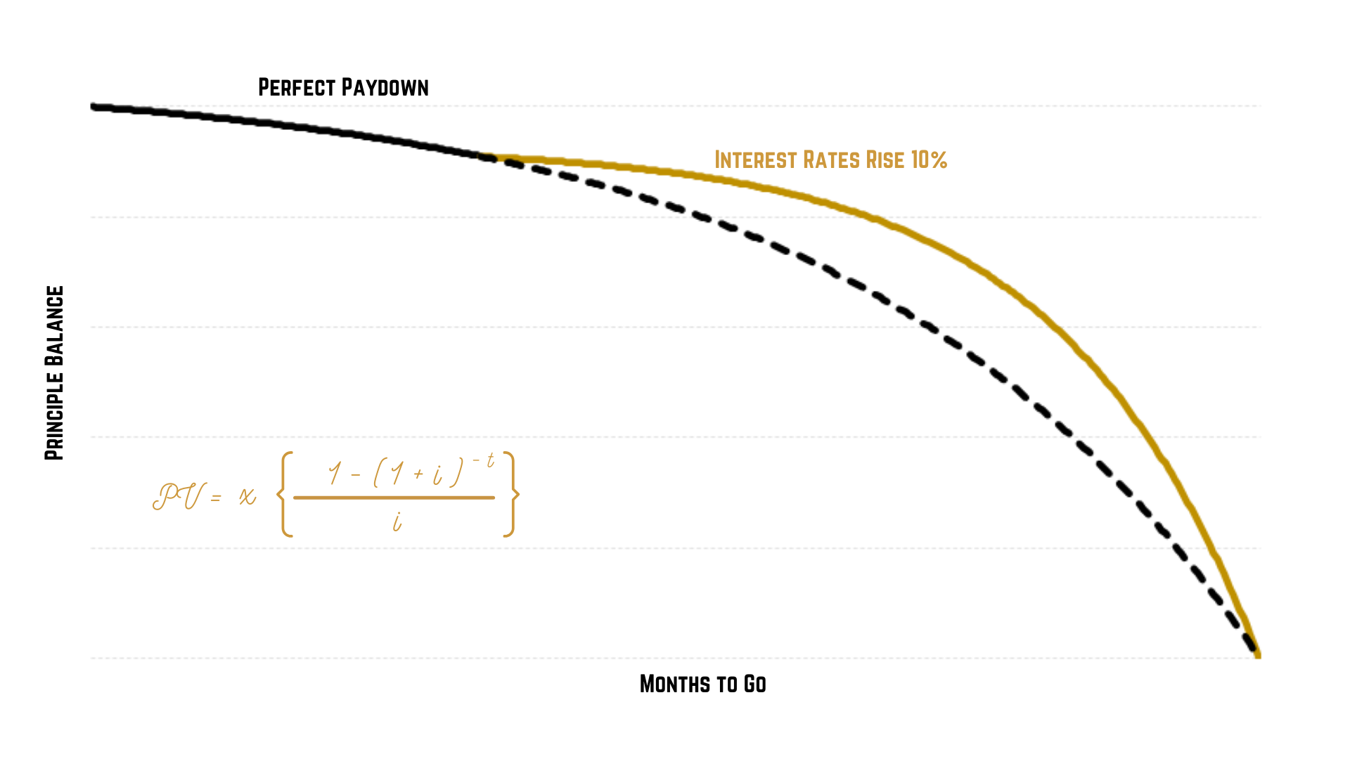
Perfect paydown curves
Although from a customer’s point of view the monthly repayments on a loan remain the same over time, from a lender’s point of view the ratio between revenue earned and principal paid downfalls over time, following the exponential shape of an annuity curve.
This is due to the nature of compound interest. In the early months, the majority of each payment goes towards the interest, leaving only a small amount to chip away at the principal debt. However, with each payment received the balance decreases slightly, leaving more and more for the principal balance.
The mathematical equation that describes this curve is shown below:
PV = x [ (1 – (1 + i) -t )/ i ]
Where:
PV = the present value of the loan at a given point in time
x = the instalment amount
i = the interest rate
t = the number of terms remaining
You can shuffle this all around as needed, so that: if the PV is lower than the actual balance outstanding, a customer is in arrears (in the old days I had to do this sometimes when we took on portfolios with questionable data hygiene but that’s seldom needed these days); if in collections, you need to reduce the instalment by a certain amount, you can see how many months the loan would be extended by; or, in the affordability context; if you have calculated the maximum monthly instalment and have a set term and price, what the largest affordable loan is.
Assigning Initial Loan Sizes
The first step is to estimate a customer’s monthly free cash flow, which isn’t always easy but is getting easier with tools like Open Banking. I’ve written elsewhere about the mechanics of affordability and where it differs from risk, so for the sake of brevity here I’ll just assume a customer has €5 000 a month of free cash flow after all current expenses have been paid, and the lender in question allows 50% of free cash flows to be used as a monthly loan repayment.
We can then pop €2 500 into the equation and solve for PV, which at this point would be the initial loan amount. Assuming the lender wishes to make the loan over a one-year period at 10%, they should lend the customer in question no more than € 28 436, for example.
The result of the annuity formula would then be passed through a second set of filters to ensure that the loan offered did not contravene product parameters or regulations – perhaps the customer qualifies for €28 436 according to the maths, but if the lender never makes first loans for more than €25 000 to new customers, the offer would be decreased at this stage to €25 000.
In more sophisticated operations the annuity model method can also be used to accommodate risk-based loan assignments. It used to be the case that the easiest way to do this was by adjusting the proportion of free cash flow set aside for loans. So, a customer with a strong affordability score – where those exist – might be allowed to use 60% of their free cash flow in the example above, while a customer with a weak affordability score might only be allowed to use 30%.
Keeping everything else the same, the customer with strong affordability would qualify for €34 124, the customer with affordability concerns just €17 062.
And of course, the product itself would influence the calculation, with secured loans and especially mortgages generally accepting larger shares of the free cash flows. Now, though, with the advent of buy now pay later, we also have the opportunity to use the individual transaction in a similar way. There is a delicate balance between protecting customers and being paternalistic, but one of BNPL’s biggest criticisms is that it encourages frivolous items to be paid off on credit – but this could also be its biggest strength since each individual credit extension is made with the full knowledge of what it is being used for, so we could have a situation where different affordability ratios are applied for different categories of goods.