
An Interpretable Machine Learning Model for Daily Global Solar Radiation Prediction
by
Mohamed Chaibi
1,*, 
EL Mahjoub Benghoulam
1,
Lhoussaine Tarik
2,
Mohamed Berrada
3 and
Abdellah El Hmaidi
4 1
Team of Renewable Energy and Energy Efficiency, Department of Physics, Faculty of Science, University of Moulay Ismail, Zitoune, Meknes BP 11201, Morocco
2
Water and Environmental Engineering Laboratory, Faculty of Science and Technique, Mining, University of Moulay Ismail, Boutalamine, Errachidia BP 509, Morocco
3
Laboratory of Mathematical and Computational Modeling, ENSAM, University of Moulay Ismail, Marjane II, Al Mansour, 50000, Meknes BP 15290, Morocco
4
Laboratory of Water Sciences and Environmental Engineering, Department of Geology, Faculty of Science, University of Moulay Ismail, Zitoune, Meknes BP 11201, Morocco
*
Author to whom correspondence should be addressed.
Energies 2021, 14(21), 7367; https://doi.org/10.3390/en14217367
Submission received: 18 September 2021
/
Revised: 24 October 2021
/
Accepted: 27 October 2021
/
Published: 5 November 2021
Abstract
:Machine learning (ML) models are commonly used in solar modeling due to their high predictive accuracy. However, the predictions of these models are difficult to explain and trust. This paper aims to demonstrate the utility of two interpretation techniques to explain and improve the predictions of ML models. We compared first the predictive performance of Light Gradient Boosting (LightGBM) with three benchmark models, including multilayer perceptron (MLP), multiple linear regression (MLR), and support-vector regression (SVR), for estimating the global solar radiation (H) in the city of Fez, Morocco. Then, the predictions of the most accurate model were explained by two model-agnostic explanation techniques: permutation feature importance (PFI) and Shapley additive explanations (SHAP). The results indicated that LightGBM (R2 = 0.9377, RMSE = 0.4827 kWh/m2, MAE = 0.3614 kWh/m2) provides similar predictive accuracy as SVR, and outperformed MLP and MLR in the testing stage. Both PFI and SHAP methods showed that extraterrestrial solar radiation (H0) and sunshine duration fraction (SF) are the two most important parameters that affect H estimation. Moreover, the SHAP method established how each feature influences the LightGBM estimations. The predictive accuracy of the LightGBM model was further improved slightly after re-examination of features, where the model combining H0, SF, and RH was better than the model with all features.
1. Introduction
Renewable energy transition will enormously benefit African countries by creating employment opportunities, protecting the environment, and promoting energy security [1]. Morocco is regarded as one of the leading African countries in renewable energy, thanks to its policies encouraging investments in renewable energies. These sources of energy are expected to generate 52% of the country’s electricity by 2030 [2]. Moreover, the Moroccan government has established a new climate strategy by ratifying the Paris Agreement, and holding the United Nations Conference of Parties (COP22) in Marrakesh in 2016 [3].
Solar energy is a sustainable energy source used widely for a variety of applications, including electricity generation, water pumping, air or water heating, and water desalination [4,5]. Global solar radiation information is critical for such applications. The most precise method of acquiring this information consists of using a radiometric measurement station running continuously for an extended period. However, in most countries, particularly in Morocco, these measurements are not easily accessible due to economic and technological constraints [6]. Consequently, numerous models have been developed to estimate global solar radiation, such as empirical models [7], reanalysis models [8,9], satellite-based models [10], interpolation models [11,12], and machine learning models.
Empirical models use linear or nonlinear correlations between H and other readily available meteorological data. These models are simple to implement. However, they are location-dependent, and have limited prediction accuracy [13]. Reanalysis methods estimate H by running numerical weather prediction (NWP) models using historical observations. These models generate global solar radiation time series with global coverage. Nevertheless, they have a low spatial resolution and a medium prediction ability [14]. Satellite-based models utilize images of reflected radiation to predict H. They enable continuous monitoring of solar radiation changes, but must be validated against ground-based measurements [14,15]. Finally, interpolation techniques are used to create continuous estimates for unmeasured regions using ground point observations of global solar radiation. The quality of these models is highly dependent on the number of measurements [14].
Machine learning refers to a collection of algorithms that enable systems to learn from experience and data, rather than being explicitly programmed [16,17]. The availability of massive data, the improvement in algorithms, and the increase in computer power have driven an explosion of applications of ML in a range of areas [18], and especially in solar modeling. Studies employing ML models to estimate emerged in 2003, have increased significantly since 2014, and reached a peak in 2019 [19]. Several ML models have been adopted in these studies, namely artificial neural network-based models, kernel-based algorithms, tree-based models, and fuzzy techniques [19,20].
Artificial neural network-based models are inspired by the learning procedure of biological neural systems, which consist of interconnected information-processing units called neurons [19]. These models are the most popular ML methods adopted for global solar radiation simulation [21]. Wang et al. [22] compared three artificial neural networks (ANN) models (MLP, Radial basis function (RBF), and generalized regression neural network (GRNN)), and an empirical model, for daily H estimation at 12 sites across China. They found that the MLP and RBF were the most accurate for all stations. The best results (R2 = 0.8600, RMSE = 0.5388 kWh/m2, MAE = 0.4250 kWh/m2) were achieved with an MLP model. Kaba et al. [23] developed a deep neural network (DNN) to estimate the global solar radiation at 30 stations in Turkey. The results of comparison with four empirical models demonstrated the robustness of the DNN model with an overall R2 = 0.9800, RMSE = 0.2166 kWh/m2, and MAE = 0.1694 kWh/m2.
The kernel-based models include support-vector machines and Gaussian process regression (GPR) [19]. SVR models have been extensively used for estimation, due to their good prediction accuracy and excellent stability. However, GPR models were scarcely applied in global solar radiation studies. Piri et al. [24] compared the SVR algorithms with conventional empirical methods to predict at two sites in Iran. The findings of this research highlighted that SVR models were the most suitable for H prediction. The obtained results of statistical indicators for the first site were RMSE = 0.4515 kWh/m2 and R2 = 0.9330. On the other hand, they were RMSE = 1.1180 kWh/m2 and R2 = 0.5967 for the second site. Quej et al. [25] evaluated the potential of SVR, neuro-fuzzy inference system (ANFIS), and MLP models to predict daily global solar radiation in the Yucatán Peninsula, Mexico. The researchers achieved the best performance by the SVR algorithm with R2 = 0.6890, RMSE = 2.4820 kWh/m2, and MAE = 1.9180 kWh/m2. Chen et al. [26] tested seven SVR models at three sites in China. The researchers found that all the SVR models provided a better accuracy than the empirical models with an average RMSE of 0.5816 kWh/m2. Guermoui et al. [27] estimated daily H with the GPR model in Ghardaïa, Algeria. It was concluded that the GPR model outperformed the MLP and RBF models. The obtained results in terms of the mean bias error (MBE), RMSE, normalized root mean square error (nRMSE), and correlation coefficient (r) were 0.1861 kWh/m2, 0.3194 kWh/m2, 5.2%, and 0.9842, respectively.
Tree-based models are ML techniques that use decision trees as a base model [19]. These methods have been successfully applied in many solar radiation related studies. Benouna et al. [28] compared 3 tree-based models (boosted trees, bagged trees, and random forest (RF)), 22 empirical models, and an MLP model, for estimating H in five locations in Morocco. Their results revealed the superiority of the (RF) model in terms of r, normalized mean absolute error (nMAE), and (nRMSE) that were in the range of 0.8753–0.9620, 5.84–11.81%, and 7.85–15.33%, respectively. Fan et al. [21] compared the XGBoost model with the SVR technique for predicting daily H in humid subtropical China. The authors reported that XGBoost (R2 = 0.7530, RMSE = 0.9238 kWh/m2, MAE = 0.6925 kWh/m2) exhibited a similar performance to SVR while outperforming the empirical models.
Fuzzy logic techniques take into account the uncertainty associated with weather conditions to estimate H [29]. Boata et al. [30] proposed a functional fuzzy approach to forecast daily global solar radiation at 12 European stations. The results of RMSE and MAE were between 1.04–1.69 kWh/m2 and 0.66–1.16 kWh/m2., respectively. Rizwan et al. [29] used a fuzzy logic approach to estimate monthly mean H in four Indian stations. They concluded that the proposed model provided a good predictive performance compared to a clear sky and MLP models, with an overall mean absolute percentage error (MAPE) of 5% across all stations.
In 2017, Ke et al. [31] developed a novel tree-based ensemble method named LightGBM, which is a new variant of gradient boosting with a faster training time and higher prediction capability. This model has been successfully applied in many fields to predict the energy yield of photovoltaic systems [32], protein–ATP binding residues [33], peer-to-peer network loan default [34], and reference evapotranspiration [35]. However, LightGBM was rarely used in global solar radiation estimation. To the best of the authors’ knowledge, only Park et al. [36] used the LightGBM algorithm to predict multistep-ahead solar radiation, using data from two regions in South Korea. The findings of this research indicated that the LightGBM algorithm was more efficient than the tree-based ensemble and deep learning methods. A list of representative literature related to the comparison ML models for H prediction is depicted in Table 1.
As the reviewed literature shows, ML models are powerful tools for global solar radiation estimation. However, most of them are considered black-box models. This means that the user will have difficulty comprehending the internal logic of these models [37] To overcome these limitations, many strategies for interpretable ML have been recently developed, including partial dependence plot (PDP), local interpretable model-agnostic Explanations (LIME), accumulated local effects (ALE), permutation feature importance (PFI), and Shapley additive explanations (SHAP) [38]. These methods can be used to explain model predictions, extract knowledge, and enhance predictive ability [39]. The explanation techniques can be classified into model-agnostic and model-specific. Model-agnostic can be applied to any ML algorithm (e.g., PFI, PDP, SHAP), while model-specific is limited to specific model classes [37]. For instance, the interpretation of regression weights in a linear model is model-specific, and does not apply to any other model [40]. Alternatively, these techniques might be classified by whether they produce global or local interpretations. Global interpretation refers to understanding the overall relationship between features and the target based on the entire model (e.g., PFI), whereas local interpretations focus on explaining the prediction of a single or a subset of instances (e.g., LIME) [38].
In solar modeling, the most popular approach for explaining predictive ML algorithms is feature importance. This strategy aims at identifying the most relevant features for global solar radiation estimation. Alsina et al. [41] used the automatic relevance determination method (ARD) to identify the most significant attributes for an ANN model developed to predict the monthly solar radiation in Italy. The group achieved the best results (mean absolute percentage error (MAPE) equal to 1.67%, an nRMSE of 1.01%, and a mean percentage bias error (MPBE) of 0.03%) with seven inputs, namely top of atmosphere radiation, day length, number of rainy days, rainfall, latitude, period of time, and altitude. Shamshirband et al. [42] conducted a sensitivity analysis for an extreme learning machine (ELM) algorithm to find the most influential input on H estimation. The results indicated that the most critical single input parameter is the relative sunshine duration, and that the optimal combination of two inputs is the sunshine duration and the difference between the maximum and minimum temperatures. Rohani et al. [43] showed, using the GPR model, that sunshine fraction duration, mean temperature, relative humidity, and extraterrestrial radiation are the most important features for daily and monthly prediction in Mashhad, Iran. Using the random forest (RF) model, Zeng et al. [44] demonstrated that daily sunshine duration, daily maximum land surface temperature, and day of the year are the most effective input variables for estimating across China.
PFI is a new global model-agnostic explanation technique that was recently used to identify the most relevant features in many fields, such as medicine [45], agriculture [46], and engineering [47]. Similarly, the SHAP method has been applied successfully to interpret local and global ML predictions in several studies in order to predict the risk of water erosion [48], estimate pairwise acquisition [49], investigate the factors that contribute to freight truck-related crashes [50], estimate the occurrence of benthic macroinvertebrate species [51], and predict the fuel properties of the chars [52].
As this brief review indicates, the application of LightGBM for global solar radiation prediction remains limited. In addition, PFI and SHAP methods have not yet been applied in H modeling to the knowledge of the authors. For this reason, this study aims:
- (1)
- To compare the performances of the newly LightGBM model to three benchmark machine learning algorithms, namely MLP, MLR, and SVR.
- (2)
- To explain the predictions of the best algorithm with PFI and SHAP techniques by quantifying the relevance of inputs, elucidating their impacts on each individual estimation, and highlighting their interaction.
- (3)
- To evaluate the efficacy of the two explanation techniques by feature re-examination of the most accurate model.
The remaining of this paper is structured as follows: Section 2 presents an overview of the different models and techniques used in this paper. It also describes the study area, data collection, partitioning process, and statistical indicators. The results are presented and discussed in Section 3. Finally, Section 4 provides the main conclusions.
2. Materials and Methods
2.1. Predictive and Explanation Techniques
2.1.1. Support-Vector Regression (SVR)
SVRs are kernel ML techniques based on statistical learning theory and the structural risk minimization principle. The fundamental idea behind SVRs is to convert the non-linear relationship between features and the target in the original space into a linear regression in a new higher dimensional space, using a process called the kernel trick [53]. More details about the SVR model can be found in [54]. The SVR model includes hyperparameters that can be tuned to reduce model overfitting and improve prediction efficiency. The hyperparameters considered in this study are (1) (C): the regularization parameter, and (2) (epsilon): the width of the tube around the estimated function.
2.1.2. Multilayer Perceptron (MLP)
MLP models are a subclass of feedforward ANNs that consist of an input layer, an output layer, and one or several hidden layers. The model first propagates the signal forward from the input layer to the hidden layer and finally to the output layer. Further, the error signal is backpropagated to the input layer. A learning algorithm adjusts the network’s weights and bias until the error reaches an acceptable level. More details about this model can be found in [55]. For an MLP model with one hidden layer, the optimized hyperparameters include (1) (activation): the activation function for the hidden layer, (2) (solver): the learning algorithm, and (3) (hidden_layers_sizes): the number of neurons in the hidden layer.
2.1.3. Multiple Linear Regression (MLR)
MLR model is based on a linear relationship between the features, , and the output variable, , given as [56]:
where is the intercept, , … are regression coefficients, and is the number of features.
2.1.4. Light Gradient Boosting (LightGBM)
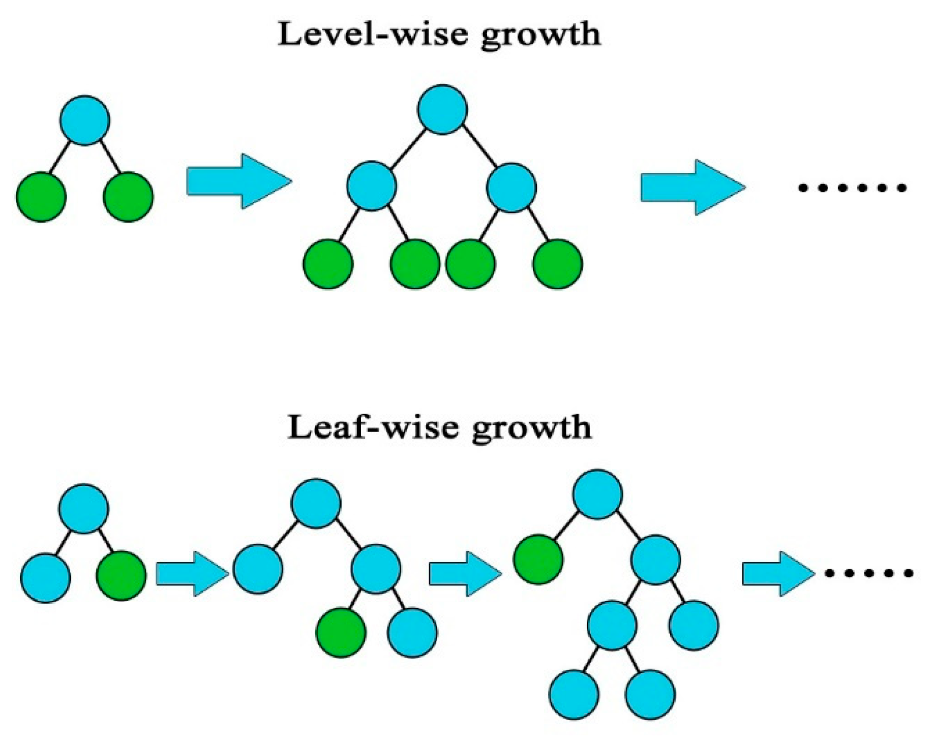
LightGBM is a variant of gradient boosting proposed by Ke et al. [31] in 2017. Gradient boosting refers to an ensemble model based on a decision tree as a weak learner. The predictive ability and the computational cost of this algorithm deteriorate when a large amount of data is available, or the attribute dimension is high. The LightGBM model can overcome these limitations by using gradient-based one-side sampling (GOSS) and exclusive feature bundling (EFB) techniques [57]. Furthermore, the LightGBM model grows its trees using the leaf-wise strategy, rather than the level-wise tree technique. This strategy grows the trees vertically, whereas other algorithms grow them horizontally. Figure 1 illustrates the two tree growth strategies.
Due to its high sensitivity to overfitting, the LightGBM’s hyperparameters should be optimized. The main hyperparameters of this model are (1) (num_leaves): the number of leaves per tree, (2) (learning_rate): the parameter that controls the speed of iteration, and (3) (max_depth): the maximum depth of the tree. More details about the LightGBM algorithm can be found in [31].
2.1.5. Permutation Feature Importance (PFI)
PFI was proposed by Breiman for random forests, and extended for all ML models by Fisher et al. in 2018 [58]. The basic idea is to permute the values of a variable , and calculate how much the prediction error increases because of this permutation. The computation of the PFI score comprises the following four steps: (1) estimation of the original model error , (2) permutation of the values of the predictor variable , (3) calculation of the new error , and (4) determination of the permutation feature importance score [38]. The error used in this paper is the mean absolute error (MAE) defined by Equation (10).
2.1.6. Shapley Additive Explanations (SHAP)
SHAP is an explanation technique introduced by Lundberg and Lee in 2017, based on cooperative game theory [59]. It calculates the individual contribution of each feature using Shapley values [60], where the Shapley value corresponds to the average marginal impact of a feature value on the predictions over all feasible coalitions [59].
Let the ML model that needs to be explained,, is the explanatory model, and and denote the input variable and the simplified input, respectively. To interpret the output of the ML model, SHAP utilizes an additive feature attribution [61] as:
where is the number of attributes, is the SHAP value of a feature and represents the constant value when all input variables are missing.
SHAP can be used for both local and global explanations. The local explanations are aggregated to generate the global explanation by averaging the absolute Shapley values per feature across the data. The SHAP method is also able to identify how each feature influences the estimations (positively or negatively), and to quantify the interaction between two variables, and [59,61].
2.2. Study Area and Data Processing
2.2.1. Case Study and Data Collection
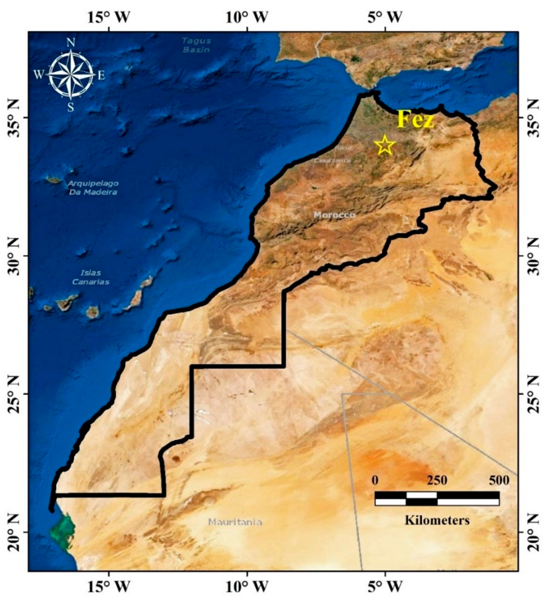
The present study used daily global solar radiation , sunshine duration , average temperature , atmospheric pressure , relative humidity , precipitation , and wind speed . These data were collected from a meteorological station in Fez (latitude 33°55′58″ N, longitude 4°58′30″ W, altitude 571.3 m) between 2016 and 2017. Figure 2 shows the location of the meteorological station. The daily extraterrestrial solar radiation () and the daily sunshine duration fraction () were added to the database as a part of the feature engineering process. The daily extraterrestrial solar radiation on a horizontal surface . is computed as [62]:
where is the solar constant, assumed equal to 1367 W/m2, is the latitude, is the day number, is the declination angle, and is sunset hour angle.
and are calculated as following:
The sunshine duration fraction is expressed as:
where and represent measured and calculated sunshine duration, respectively. The theoretical sunshine duration is given as:
The dataset contains some incorrect and missing values that must be removed. To ensure that the developed models are highly accurate, each observation must satisfy the following conditions: the daily clearness index () and should be in the ranges of and , respectively [25,62]. Among the 731 daily data used in this study, we detected five days with missing values, and four days with incorrect values.
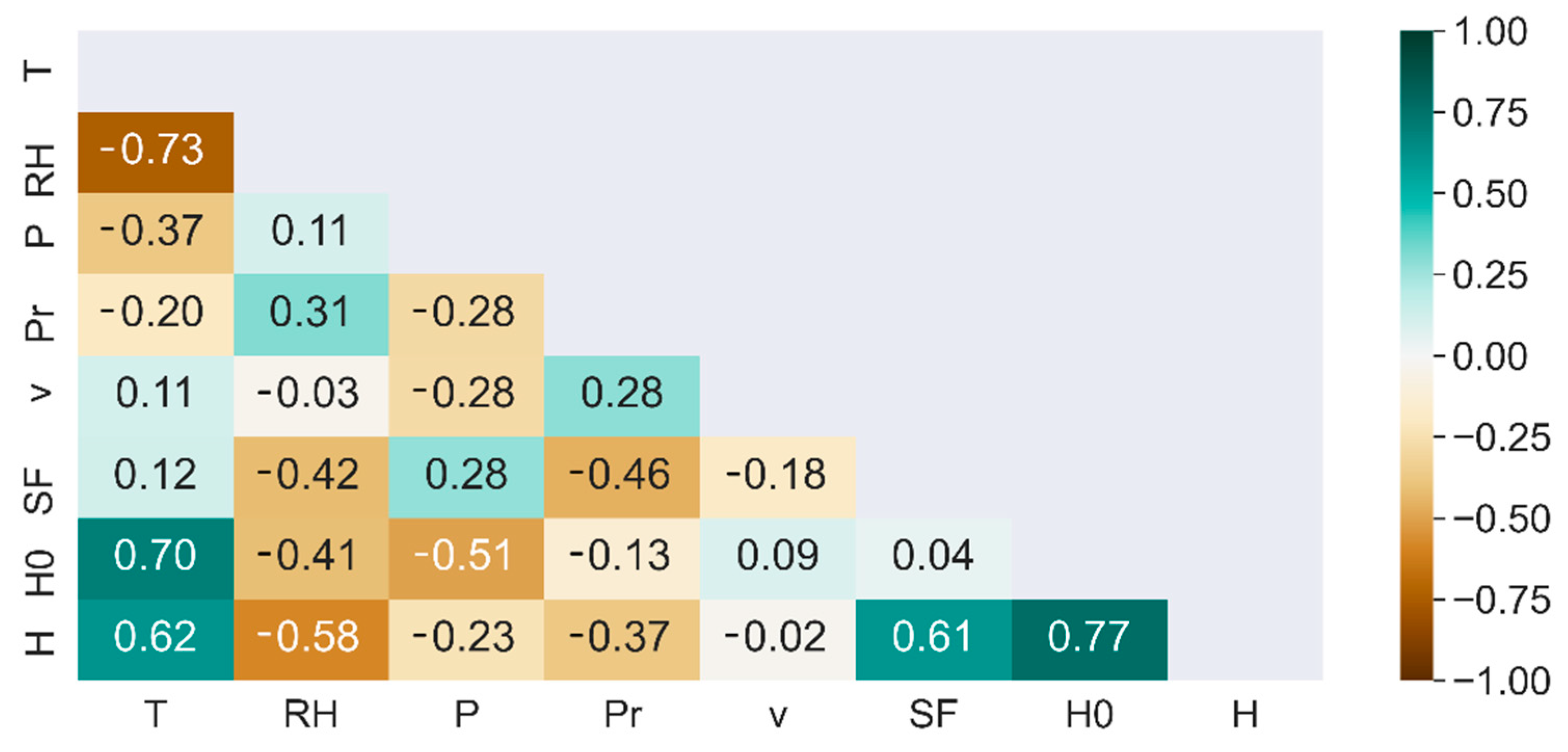
Figure 3 illustrates the triangular correlation heatmap showing the Pearson correlation coefficient r between two variables. We can see from this figure the existence of a strong positive linear correlation between and , and a moderate positive linear correlation between both features and , and . On the other hand, there is a weak negative linear association between and , a low negative linear relationship between and , and a moderate negative linear correlation between and . There is no linear relationship between and .
2.2.2. Data Preprocessing and Performance Criteria
To develop the ML models, the dataset was randomly divided into two subsamples: 60% for training, and 40% for testing. LightGBM does not require data normalization. However, the data used for MLP, MLR, and SVR must be pre-processed. The normalization formula is given as [63]:
where represent the normalized value, the real value, the maximum, and the minimum values, respectively.
The Bayesian optimization (BO) approach was used to find the optimal hyperparameters for SVR, MLP, and LightGBM machine learning models. After obtaining the hyperparameter values by running the BO algorithm 30 times, a final model was trained and tested. SVR, MLP, MLR, and PFI were developed using scikit-learn 0.24.2, LightGBM was developed using LightGBM 3.2.1.99, SHAP was implemented using SHAP, and the Bayesian optimization was implemented using scikit-optimize libraries in Python 3.8.9.
Three statistical indicators were selected to evaluate the robustness of the developed models, namely root mean square error (RMSE), mean absolute error (MAE), and the coefficient of determination (R2) defined as [64]:
where is the number of observations, denotes the calculated solar radiation, represents the measured solar radiation, and is the mean of the measured solar radiation values.
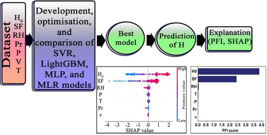
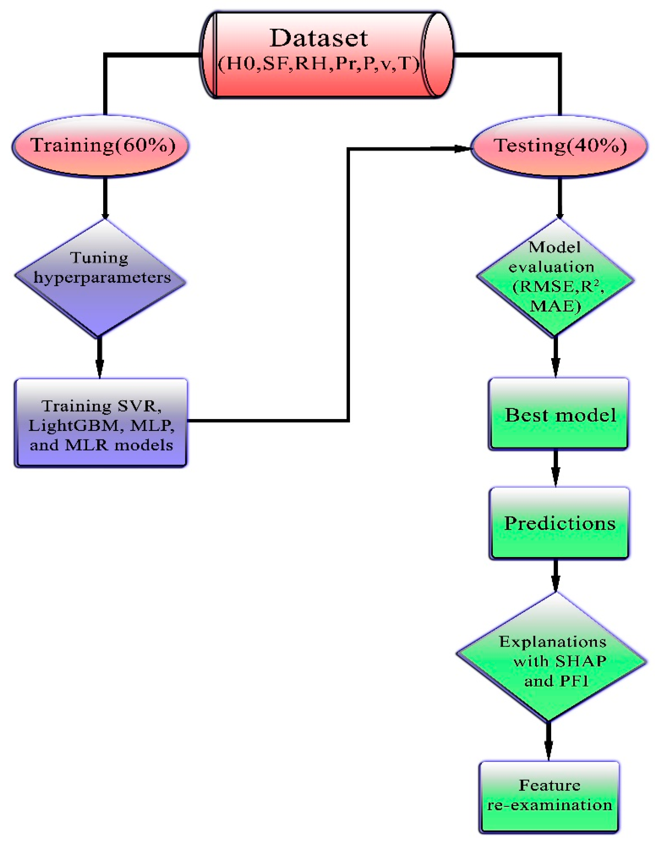
A model achieves high predictive accuracy when RMSE and MAE are close to 0 and R2 is close to 1. The methodology used in this study is illustrated in Figure 4.
3. Results and Discussion
In the next section, we tuned the hyperparameters of the three algorithms, SVR, MLP, and LightGBM, using the Bayesian optimization approach. Then, we compared SVR, MLP, MLR, and LightGBM to choose the most accurate of them.
3.1. Predictive Performance of the ML Models
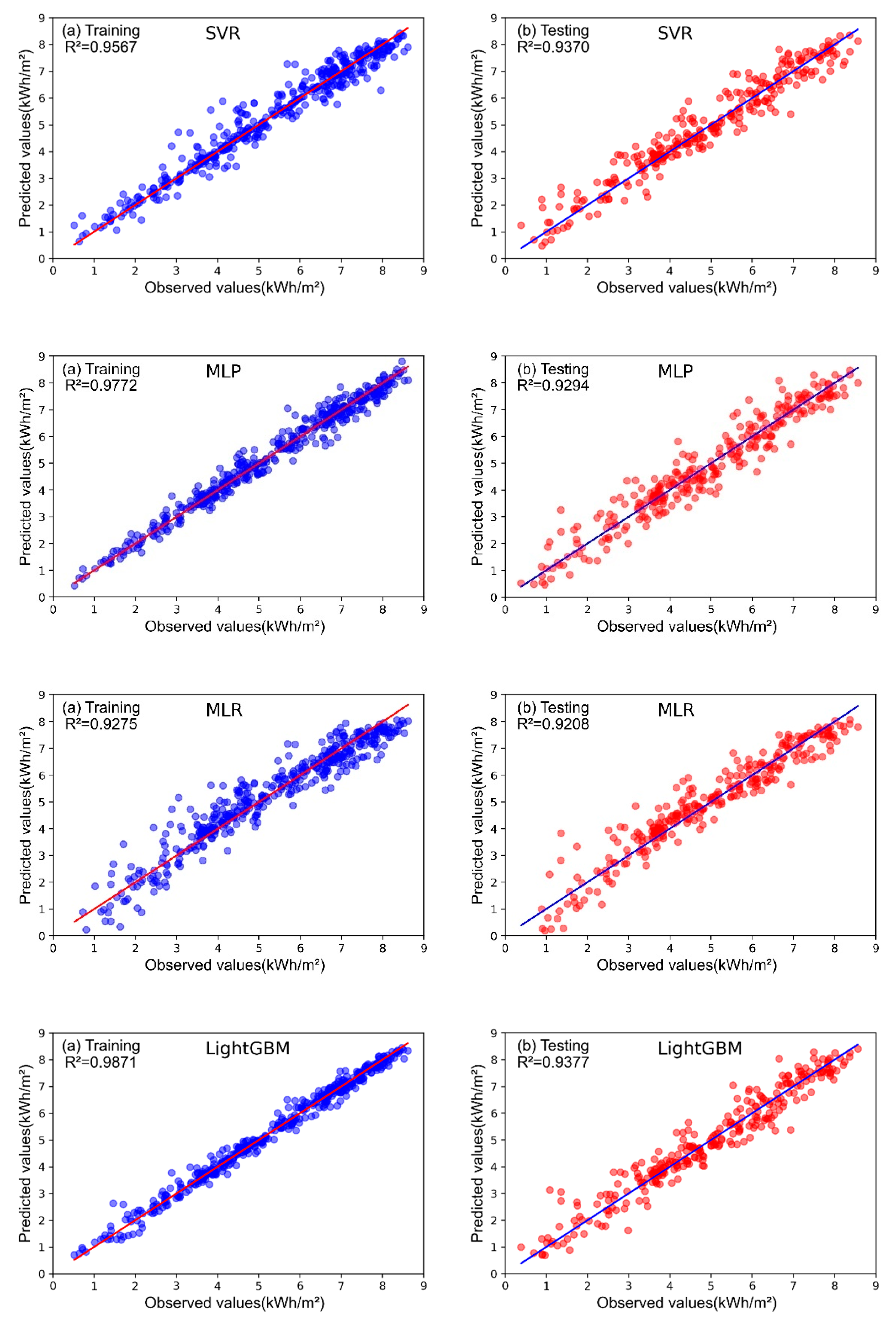
Table 2 summarizes the optimal hyperparameters for the SVR, MLP, and LightGBM models. The values of the statistical indicators obtained by SVR, MLP, MLR, and LightGBM models during the training and testing stages are depicted in Table 3. According to this table, the performances obtained by LightGBM (R2 = 0.9871, RMSE = 0.2229 kWh/m2, MAE = 0.1638 kWh/m2) in the training phase were significantly better than those of MLR (R2 = 0.9275, RMSE = 0.5290 kWh/m2, MAE = 0.3955 kWh/m2), and superior than those of SVR (R2 = 0.9567, RMSE = 0.4089 kWh/m2, MAE = 0.2697 kWh/m2) and MLP (R2 = 0.9772, RMSE = 0.2968 kWh/m2, MAE = 0.2208 kWh/m2) models. In the testing phase, LightGBM (R2 = 0.9377, RMSE = 0.4827 kWh/m2, MAE = 0.3614 kWh/m2) exhibited comparable prediction performance with SVR (R2 = 0.9370, RMSE = 0.4855 kWh/m2, MAE = 0.3639 kWh/m2), and outperformed the MLP (R2 = 0.9294, RMSE = 0.5140 kWh/m2, MAE = 0.3924 kWh/m2) and MLR (R2 = 0.9208 RMSE = 0.5443 kWh/m2, MAE = 0.4023 kWh/m2) models.
Figure 5 presents the scatter plots of the predicted daily global solar radiation values using the three ML models against the measured values during training and testing phases. As shown in this figure, the plotted data points in the training stage are generally located near the 1:1 line for MLP and LightGBM algorithms, while they are more scattered in the case of MLR. In the testing stage, the four techniques yielded more scattered estimates, particularly the MLR model.
Since LightGBM was the most accurate model, the analysis with PFI and SHAP approaches was restricted to this algorithm. Based on the results of these two techniques, a re-examination of the LightGBM model’s features was conducted to enhance its predictive performance.
3.2. Feature Importance Using PFI
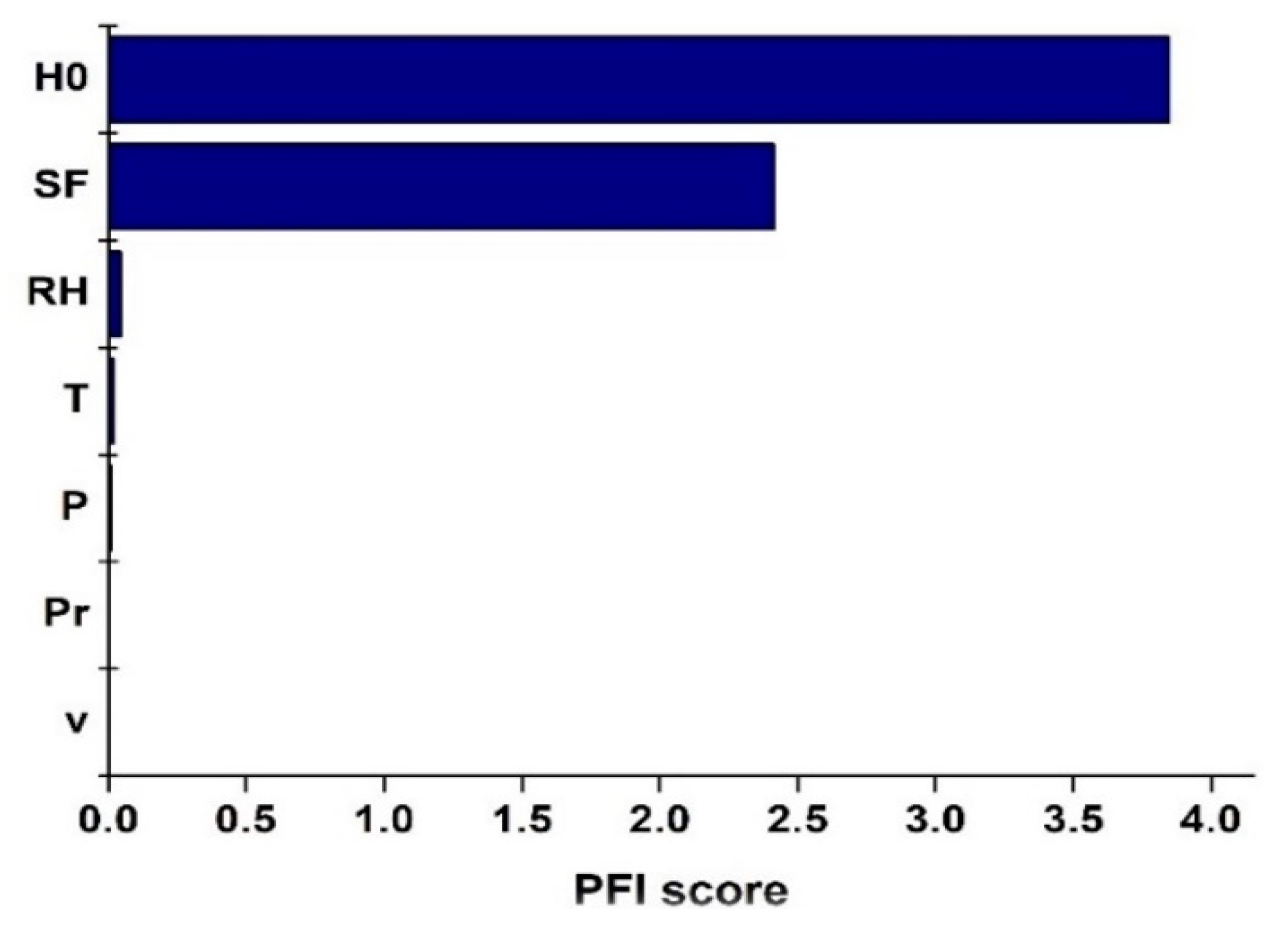
In this section, we used the PFI technique to determine the importance of each feature for estimation, and to identify the most effective of them. Figure 6 represents the PFI scores of the seven investigated predictors. Among all features, and were the most important, with PFI scores of 4 and 2.39, respectively. These two variables are widely used in solar modeling, since and are deterministic parameters calculated using sun geometry equations, and sunshine duration data are available in most meteorological stations worldwide [65]. Traditionally, these two quantities represented the components of the linear or nonlinear Angström–Prescott models, where is used as an independent variable, and is part of the clearness index ratio [66]. The next three relevant parameters , , and P had low PFI scores with values of 0.046, 0.019 and 0.01, respectively. The remaining attributes had insignificant PFI scores.
3.3. Local and Global Explanations Using SHAP
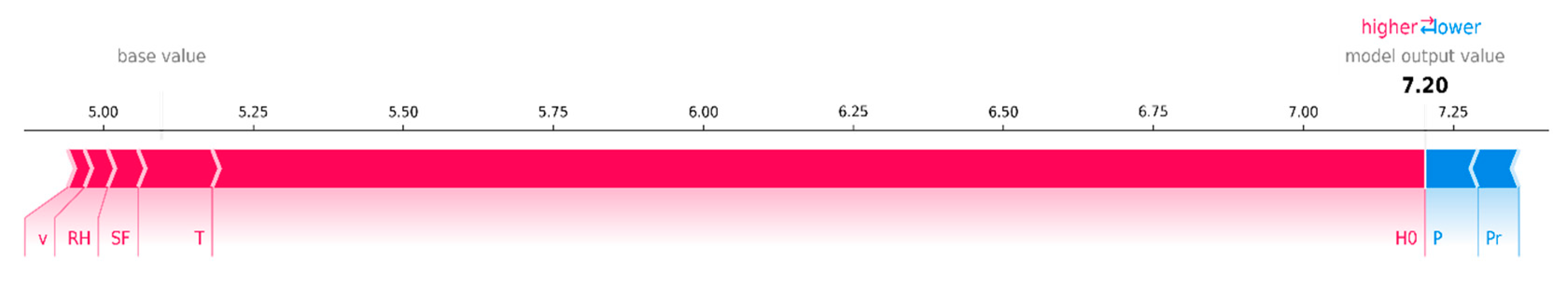
The PFI method offers global explanations by identifying the most important attributes. In contrast, the SHAP method can provide both local and global explanations. SHAP explains the outcomes of individual observations, quantifies the relative importance of features, and elucidates their influence on model prediction. Figure 7 shows the explanation generated by the SHAP method for an instance chosen randomly from the testing dataset. The base value (5.097) represents the mean model prediction over the testing dataset. Predictors that move the estimation higher than the base value (to the right) are in red, while those moving it lower are in blue. Table 4 shows the feature values for this observation, as well as the contribution of features to the LightGBM model’s output value of 7.20.
It can be seen from Figure 8 and Table 4 that demonstrated the highest contribution, whereas showed the lowest one. Moreover, , , , and pushed the prediction to the right with values of 2.02, 0.05, 0.04, 0.12, and 0.03 respectively. On the other side, and pushed the prediction to the left by −0.09 and −0.07, respectively. As a result, the estimated output value was given as follows:
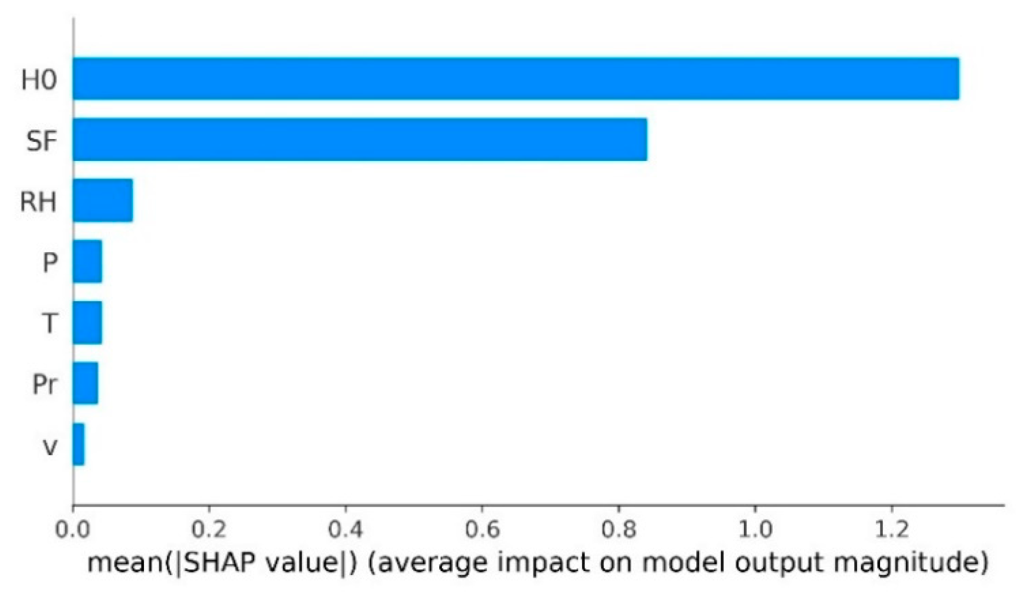
To generate a global interpretation of the LightGBM predictions, the local interpretations were aggregated by averaging the absolute Shapley values per attribute across the data. Figure 8 represents the SHAP feature importance plot which shows the global effect of each feature on estimation. The SHAP method confirmed that and are the most important features, and that is the least effective feature. This method also confirmed the order of importance of the five features , , , , and . However, it reversed the order of and .
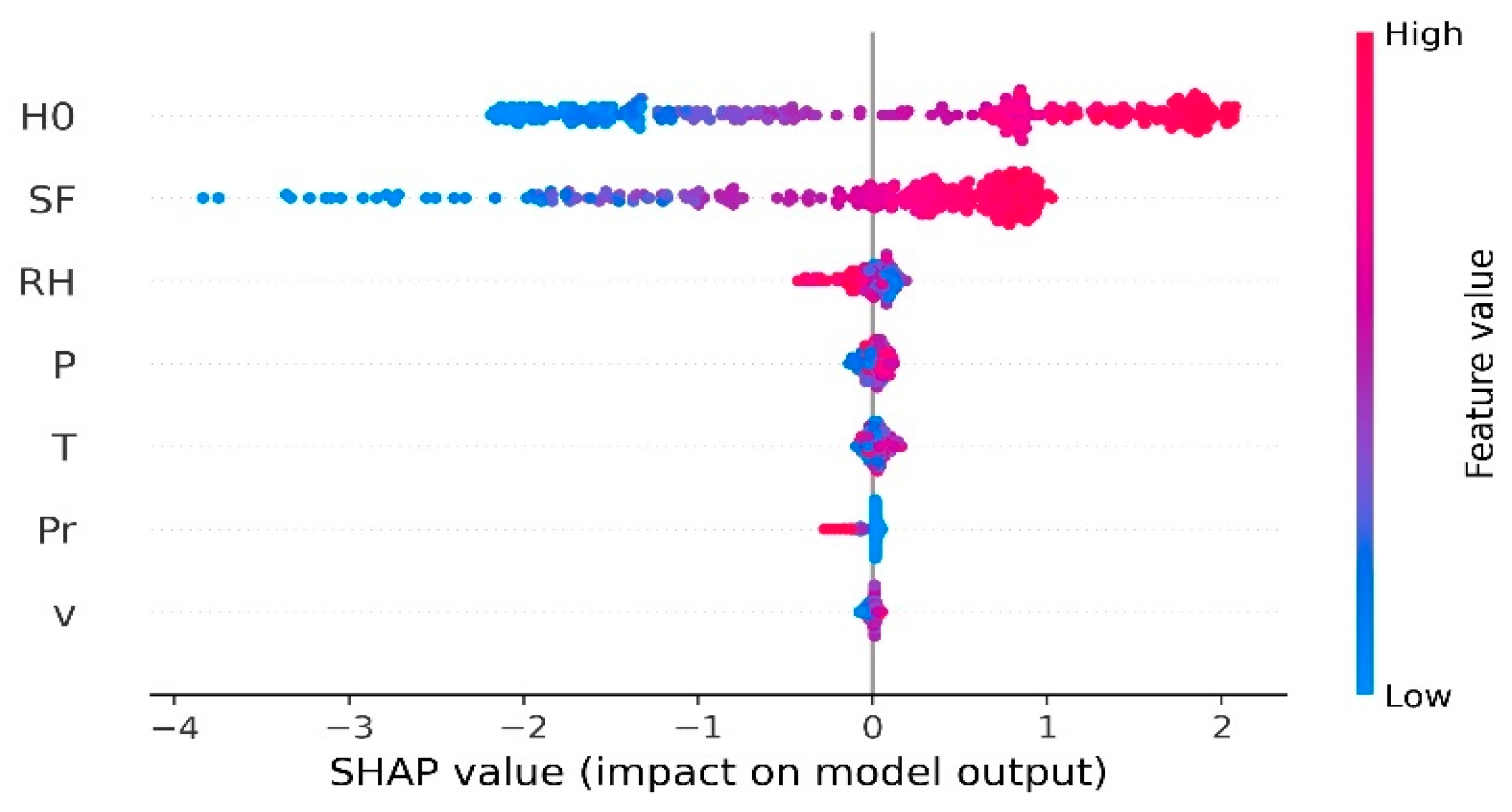
We used the SHAP summary plot (Figure 9) to determine the magnitude and direction of each attribute’s impact at global and local scales. This plot contains many points, where the y-axis indicates the feature names in decreasing order of relevance, and the x-axis indicates the SHAP values for each input predictor. Red points correspond to higher values of the feature, while blue points to lower ones.
We can observe from this plot that and showed a high positive association with estimation. This is consistent with the scientific knowledge and the results of Section 2.2.1, which indicate the existence of a direct correlation between these two quantities and : the solar radiation reaching the ground is the fraction of that is transmitted through the atmosphere, and is an indirect index of the sky’s state, where higher values of correspond to clear days and lower values correspond to overcast days [65]. This figure also revealed that the highest values of had the maximum positive impact on prediction. On the other hand, the lowest values of had the highest negative impact.
was inversely related to prediction for the majority of examples, with higher values of this feature leading to lower SHAP values and vice versa. and had comparable influences on estimation, and exhibited a mixed pattern, where different values of these attributes are associated with both high and low impacts on the predictions. Insignificant positive SHAP values were recorded for low values of , and a small negative impact on prediction was produced when increased. The wind speed was the least relevant feature, with no significant effect on prediction.
3.4. Feature Dependency Analysis
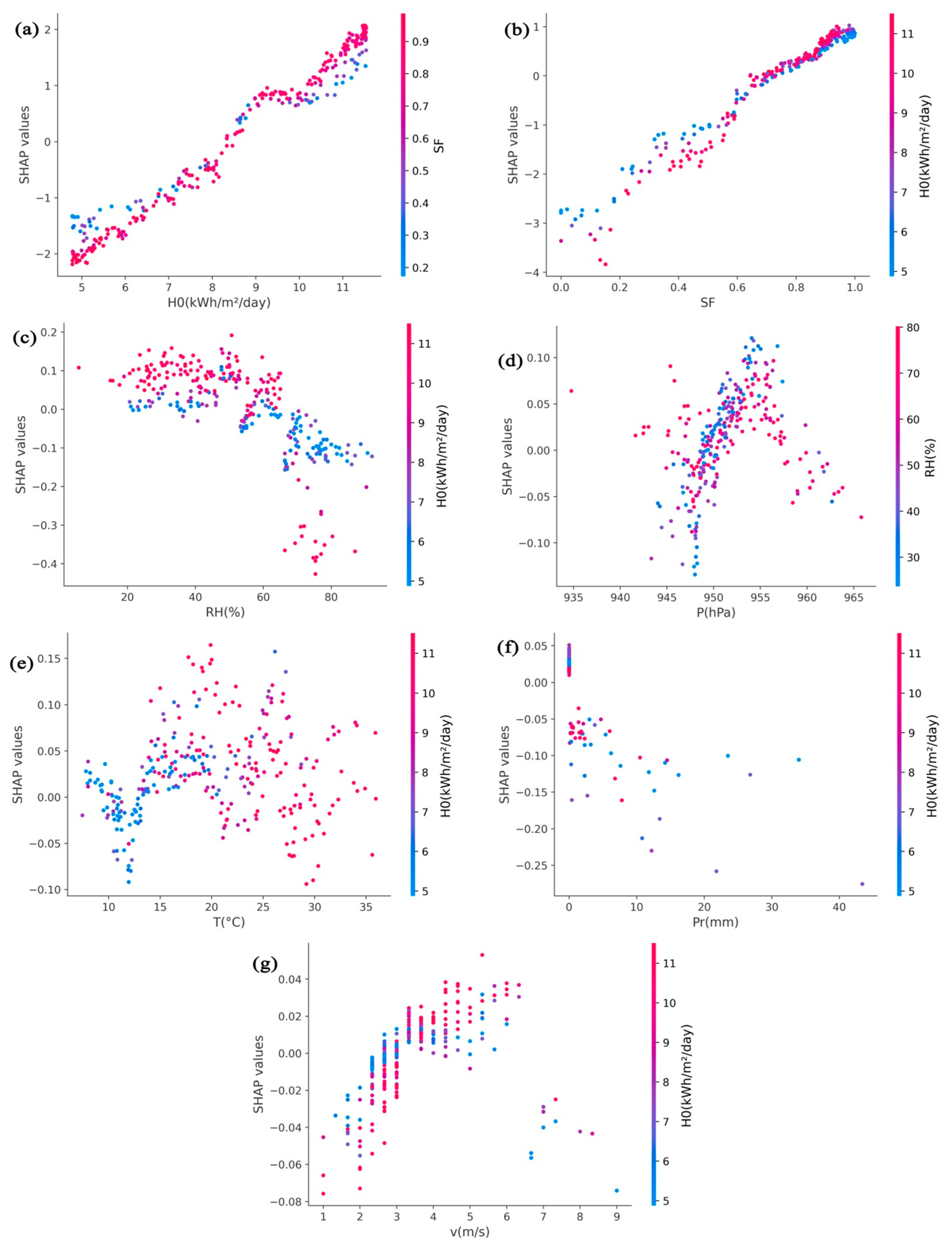
To get more insight into the LightGBM’s behavior when predicting , we used the SHAP partial dependence plots for the seven predictor variables (Figure 10). Each plot illustrates how the values of a feature (x-axis) affect the prediction (y-axis) of each instance in the dataset [67]. The plots also include another feature that the selected variable interacts most with.
We can see from this figure that had the highest interaction with all other features, with the exception of which interacted strongly with . We can also see from Figure 10a,b the existence of a positive trend between the features and , and estimation. These two features had the highest interaction between them, and generated a positive impact on prediction when .34 kWh/m2 or > 0.64, and vice versa. The feature interaction caused the spread of SHAP values for these attributes where a larger negative influence was produced when or was smaller, whereas the other predictor was larger, and a high positive impact was generated when these two features varied in the same direction.
Figure 10c depicts the relationship between SHAP values and relative humidity. According to this figure, SHAP values were generally positive when < 57%, and became completely negative when RH exceeded 65.4%, with the maximum negative impact observed when is in the range 70–80% and kWh/m2.
The influences of and on LightGBM predictions are shown in Figure 10d,e. As can be seen from these figures, no obvious relationship exists between and and the SHAP values. On the other hand, when < 943 hPa or 951 hPa < < 957.2 hPa, a purely positive impact on H estimation was produced, while a purely negative influence was generated when > 961 hPa. The average temperature had a purely positive impact on global solar radiation estimation when 13.4 < < 19.8 , and a mixed impact for the other values.
Figure 10f indicates that, for low values of precipitation (, a small positive effect on global solar radiation estimation was produced; this effect peaked at medium values of . When was above zero, the effect became negative.
Figure 10g shows that wind speed engendered a minor purely negative impact on estimation when < 2.33 m/s or > 6.7 m/s. In contrast, a minor purely positive influence was recorded when 3.2 m/s < < 4.9 m/s or 5.2 m/s < < 6.4 m/s.
3.5. Feature Re-Examination of LigtGBM
The two techniques, PFI and SHAP, showed that the input variables had different impacts on estimation, and that some of them were redundant. Besides, the SHAP method quantified the interaction between the features. To assess the effectiveness of these two explanation techniques, we compared the LightGBM model with all inputs to seven LightGBM models using the top three most relevant features. Table 5 shows the obtained results during the testing phase. According to this table, was the best single input, followed by , and then . This ranking agrees with the results obtained by PFI and SHAP methods. The model integrating and as predictors showed close results (R2 = 0.9336, RMSE = 0.4984 kWh/m2, MAE = 0.3700 kWh/m2) to the model with complete features, and performed significantly better than both models combining the two features ( or (. These results confirmed that and are the most interactive and the most important for estimation. The model associating , , and (R2 = 0.9382, RMSE = 0.4806 kWh/m2, MAE = 0.3602 kWh/m2) slightly outperformed the model with all variables. This model achieved a reasonable prediction accuracy compared to the results reported in the literature (Table 1). For instance, the performances are comparable or better than those obtained in [21,22,24,25,26]. On the other hand, they are worse than those reported in [23,27].
These findings proved the benefits of the interpretation techniques, particularly the SHAP method, for understanding the inner working of ML models and boosting their predictive capability. Nonetheless, some limitations to our study should be acknowledged, such as the small sample size of the dataset, and its restriction to one geographical location. Thus, further research should be conducted using more data collected over different locations.
4. Conclusions
In this paper, we started by comparing four ML models for predicting global solar radiation in Fez, Morocco. The results revealed that the LightGBM had comparable performances with SVR, and outperformed the MLP and MLR models. The LightGBM’s predictions were then explained by two model-agnostic interpretation techniques. Both the PFI and SHAP methods showed that and are the most important features for estimating global solar radiation. Moreover, the SHAP model was able to highlight the effect of each attribute on estimation, and to provide local explanations. The predictive ability of the LightGBM model was further slightly improved by feature re-examination based on the results of the two explanation techniques. The findings of this paper proved the utility of using interpretation strategies to explain and enhance the predictive performance of ML models. Additional assessment is required on the applicability of these interpretation approaches to explain the estimations of other predictive ML models, as well as the use of other interpretation strategies, such as local interpretable model-agnostic explanations (LIME), accumulated local effects (ALE), and partial dependence plots (PDP).
Author Contributions
Conceptualization, M.C. and E.M.B.; methodology, M.C., L.T. and M.B.; modelling, M.C., L.T. and M.B.; validation, E.M.B., writing—original draft preparation, M.C. and A.E.H.; supervision, A.E.H. and E.M.B.; schemes and charts, M.C. and L.T.; writing—review and editing M.C. All authors have read and agreed to the published version of the manuscript.
Funding
This research received no external funding.
Data Availability Statement
The data presented in this study are available on [Figshare] at [https://doi.org/10.6084/m9.figshare.16574708].
Acknowledgments
The authors would like to thank the Moroccan Department of National Meteorology for providing the data used in this study.
Conflicts of Interest
The authors declare no conflict of interest.
References
- The Renewable Energy Transition in Africa. Available online: https://www.irena.org/publications/2021/March/The-Renewable-Energy-Transition-in-Africa (accessed on 28 August 2021).
- Boulakhbar, M.; Lebrouhi, B.; Kousksou, T.; Smouh, S.; Jamil, A.; Maaroufi, M.; Zazi, M. Towards a large-scale integration of renewable energies in Morocco. J. Energy Storage 2020, 32, 101806. [Google Scholar] [CrossRef]
- Ghezloun, A.; Saidane, A.; Merabet, H. The COP 22 New commitments in support of the Paris Agreement. Energy Procedia 2017, 119, 10–16. [Google Scholar] [CrossRef]
- Mohammadi, K.; Shamshirband, S.; Kamsin, A.; Lai, P.; Mansor, Z. Identifying the most significant input parameters for predicting global solar radiation using an ANFIS selection procedure. Renew. Sustain. Energy Rev. 2016, 63, 423–434. [Google Scholar] [CrossRef]
- Mekhilef, S.; Saidur, R.; Safari, A. A review on solar energy use in industries. Renew. Sustain. Energy Rev. 2011, 15, 1777–1790. [Google Scholar] [CrossRef]
- Tao, H.; Ewees, A.A.; Al-Sulttani, A.O.; Beyaztas, U.; Hameed, M.M.; Salih, S.Q.; Armanuos, A.M.; Al-Ansari, N.; Voyant, C.; Shahid, S.; et al. Global solar radiation prediction over North Dakota using air temperature: Development of novel hybrid intelligence model. Energy Rep. 2020, 7, 136–157. [Google Scholar] [CrossRef]
- Halawa, E.; GhaffarianHoseini, A.; Li, D.H.W. Empirical correlations as a means for estimating monthly average daily global radiation: A critical overview. Renew. Energy 2014, 72, 149–153. [Google Scholar] [CrossRef]
- Dee, D.; Uppala, S.M.; Simmons, A.J.; Berrisford, P.; Poli, P.; Kobayashi, S.; Andrae, U.; Balmaseda, M.A.; Balsamo, G.; Bauer, P.; et al. The ERA-Interim reanalysis: Configuration and performance of the data assimilation system. Q. J. R. Meteorol. Soc. 2011, 137, 553–597. [Google Scholar] [CrossRef]
- Gelaro, R.; McCarty, W.; Suárez, M.J.; Todling, R.; Molod, A.; Takacs, L.; Randles, C.; Darmenov, A.; Bosilovich, M.G.; Reichle, R.; et al. The Modern-Era Retrospective Analysis for Research and Applications, Version 2 (MERRA-2). J. Clim. 2017, 30, 5419–5454. [Google Scholar] [CrossRef] [PubMed]
- Bamehr, S.; Sabetghadam, S. Estimation of global solar radiation data based on satellite-derived atmospheric parameters over the urban area of Mashhad, Iran. Environ. Sci. Pollut. Res. 2020, 28, 7167–7179. [Google Scholar] [CrossRef] [PubMed]
- Alsamamra, H.; Ruiz-Arias, J.A.; Pozo-Vázquez, D.; Tovar-Pescador, J. A comparative study of ordinary and residual kriging techniques for mapping global solar radiation over southern Spain. Agric. For. Meteorol. 2009, 149, 1343–1357. [Google Scholar] [CrossRef]
- Ruiz-Arias, J.; Pozo-Vázquez, D.; Santos-Alamillos, F.; Lara-Fanego, V.; Tovar-Pescador, J. A topographic geostatistical approach for mapping monthly mean values of daily global solar radiation: A case study in southern Spain. Agric. For. Meteorol. 2011, 151, 1812–1822. [Google Scholar] [CrossRef]
- Besharat, F.; Dehghan, A.A.; Faghih, A.R. Empirical models for estimating global solar radiation: A review and case study. Renew. Sustain. Energy Rev. 2013, 21, 798–821. [Google Scholar] [CrossRef]
- Urraca, R.; Martinez-De-Pison, E.; Sanz-García, A.; Antonanzas, J.; Antonanzas-Torres, F. Estimation methods for global solar radiation: Case study evaluation of five different approaches in central Spain. Renew. Sustain. Energy Rev. 2017, 77, 1098–1113. [Google Scholar] [CrossRef]
- Huang, G.; Li, Z.; Li, X.; Liang, S.; Yang, K.; Wang, D.; Zhang, Y. Estimating surface solar irradiance from satellites: Past, present, and future perspectives. Remote. Sens. Environ. 2019, 233, 111371. [Google Scholar] [CrossRef]
- Cohen, S. The basics of machine learning: Strategies and techniques. In Artificial Intelligence and Deep Learning in Pathology; Elsevier: Amsterdam, The Netherlands, 2020; pp. 13–40. [Google Scholar] [CrossRef]
- Raz, A.K.; Llinas, J.; Mittu, R.; Lawless, W.F. Engineering for emergence in information fusion systems: A review of some challenges. In Human-Machine Shared Contexts; Elsevier Science: Amsterdam, The Netherlands, 2020; pp. 241–255. [Google Scholar] [CrossRef]
- Schmidt, J.; Marques, M.R.G.; Botti, S.; Marques, M.A.L. Recent advances and applications of machine learning in solid-state materials science. Npj Comput. Mater. 2019, 5, 1–36. [Google Scholar] [CrossRef]
- Zhou, Y.; Liu, Y.; Wang, D.; Liu, X.; Wang, Y. A review on global solar radiation prediction with machine learning models in a comprehensive perspective. Energy Convers. Manag. 2021, 235, 113960. [Google Scholar] [CrossRef]
- Fan, J.; Wu, L.; Zhang, F.; Cai, H.; Zeng, W.; Wang, X.; Zou, H. Empirical and machine learning models for predicting daily global solar radiation from sunshine duration: A review and case study in China. Renew. Sustain. Energy Rev. 2018, 100, 186–212. [Google Scholar] [CrossRef]
- Fan, J.; Wang, X.; Wu, L.; Zhou, H.; Zhang, F.; Yu, X.; Lu, X.; Xiang, Y. Comparison of Support Vector Machine and Extreme Gradient Boosting for predicting daily global solar radiation using temperature and precipitation in humid subtropical climates: A case study in China. Energy Convers. Manag. 2018, 164, 102–111. [Google Scholar] [CrossRef]
- Wang, L.; Kisi, O.; Zounemat-Kermani, M.; Salazar, G.; Zhu, Z.; Gong, W. Solar radiation prediction using different techniques: Model evaluation and comparison. Renew. Sustain. Energy Rev. 2016, 61, 384–397. [Google Scholar] [CrossRef]
- Kaba, K.; Sarıgül, M.; Avcı, M.; Kandırmaz, H.M. Estimation of daily global solar radiation using deep learning model. Energy 2018, 162, 126–135. [Google Scholar] [CrossRef]
- Piri, J.; Shamshirband, S.; Petković, D.; Tong, C.W.; Rehman, M.H.U. Prediction of the solar radiation on the Earth using support vector regression technique. Infrared Phys. Technol. 2015, 68, 179–185. [Google Scholar] [CrossRef]
- Quej, V.H.; Almorox, J.; Arnaldo, J.A.; Saito, L. ANFIS, SVM and ANN soft-computing techniques to estimate daily global solar radiation in a warm sub-humid environment. J. Atmos. Solar-Terr. Phys. 2017, 155, 62–70. [Google Scholar] [CrossRef] [Green Version]
- Chen, J.-L.; Li, G.-S.; Wu, S.-J. Assessing the potential of support vector machine for estimating daily solar radiation using sunshine duration. Energy Convers. Manag. 2013, 75, 311–318. [Google Scholar] [CrossRef]
- Guermoui, M.; Gairaa, K.; Rabehi, A.; Djafer, D.; Benkaciali, S. Estimation of the daily global solar radiation based on the Gaussian process regression methodology in the Saharan climate. Eur. Phys. J. Plus 2018, 133, 1–17. [Google Scholar] [CrossRef]
- Bounoua, Z.; Chahidi, L.O.; Mechaqrane, A. Estimation of daily global solar radiation using empirical and machine-learning methods: A case study of five Moroccan locations. Sustain. Mater. Technol. 2021, 28, e00261. [Google Scholar] [CrossRef]
- Rizwan, M.; Jamil, M.; Kirmani, S.; Kothari, D. Fuzzy logic based modeling and estimation of global solar energy using meteorological parameters. Energy 2014, 70, 685–691. [Google Scholar] [CrossRef]
- Boata, R.S.; Gravila, P. Functional fuzzy approach for forecasting daily global solar irradiation. Atmos. Res. 2012, 112, 79–88. [Google Scholar] [CrossRef]
- Ke, G.; Meng, Q.; Finley, T.; Wang, T.; Chen, W.; Ma, W.; Ye, Q.; Liu, T.-Y. Lightgbm: A Highly Efficient Gradient Boosting Decision Tree. Adv. Neural Inf. Process. Syst. 2017, 30, 3146–3154. [Google Scholar]
- Ascencio-Vásquez, J.; Bevc, J.; Reba, K.; Brecl, K.; Jankovec, M.; Topič, M. Advanced PV Performance Modelling Based on Different Levels of Irradiance Data Accuracy. Energies 2020, 13, 2166. [Google Scholar] [CrossRef]
- Song, J.; Liu, G.; Jiang, J.; Zhang, P.; Liang, Y. Prediction of Protein—ATP Binding Residues Based on Ensemble of Deep Convolutional Neural Networks and LightGBM Algorithm. Int. J. Mol. Sci. 2021, 22, 939. [Google Scholar] [CrossRef]
- Ma, X.; Sha, J.; Wang, D.; Yu, Y.; Yang, Q.; Niu, X. Study on a prediction of P2P network loan default based on the machine learning LightGBM and XGboost algorithms according to different high dimensional data cleaning. Electron. Commer. Res. Appl. 2018, 31, 24–39. [Google Scholar] [CrossRef]
- Fan, J.; Ma, X.; Wu, L.; Zhang, F.; Yu, X.; Zeng, W. Light Gradient Boosting Machine: An efficient soft computing model for estimating daily reference evapotranspiration with local and external meteorological data. Agric. Water Manag. 2019, 225, 105758. [Google Scholar] [CrossRef]
- Park, J.; Moon, J.; Jung, S.; Hwang, E. Multistep-Ahead Solar Radiation Forecasting Scheme Based on the Light Gradient Boosting Machine: A Case Study of Jeju Island. Remote. Sens. 2020, 12, 2271. [Google Scholar] [CrossRef]
- Carvalho, D.V.; Pereira, E.M.; Cardoso, J.S. Machine Learning Interpretability: A Survey on Methods and Metrics. Electronics 2019, 8, 832. [Google Scholar] [CrossRef] [Green Version]
- Molnar, C. Interpretable Machine Learning. Available online: https://christophm.github.io/interpretable-ml-book/ (accessed on 28 August 2021).
- Adadi, A.; Berrada, M. Peeking Inside the Black-Box: A Survey on Explainable Artificial Intelligence (XAI). IEEE Access 2018, 6, 52138–52160. [Google Scholar] [CrossRef]
- Azodi, C.B.; Tang, J.; Shiu, S.-H. Opening the Black Box: Interpretable Machine Learning for Geneticists. Trends Genet. 2020, 36, 442–455. [Google Scholar] [CrossRef] [PubMed]
- Alsina, E.F.; Bortolini, M.; Gamberi, M.; Regattieri, A. Artificial neural network optimisation for monthly average daily global solar radiation prediction. Energy Convers. Manag. 2016, 120, 320–329. [Google Scholar] [CrossRef]
- Shamshirband, S.; Mohammadi, K.; Yee, P.L.; Petković, D.; Mostafaeipour, A. A comparative evaluation for identifying the suitability of extreme learning machine to predict horizontal global solar radiation. Renew. Sustain. Energy Rev. 2015, 52, 1031–1042. [Google Scholar] [CrossRef]
- Rohani, A.; Taki, M.; Abdollahpour, M. A novel soft computing model (Gaussian process regression with K-fold cross validation) for daily and monthly solar radiation forecasting (Part: I). Renew. Energy 2018, 115, 411–422. [Google Scholar] [CrossRef]
- Zeng, Z.; Wang, Z.; Gui, K.; Yan, X.; Gao, M.; Luo, M.; Geng, H.; Liao, T.; Li, X.; An, J.; et al. Daily Global Solar Radiation in China Estimated From High-Density Meteorological Observations: A Random Forest Model Framework. Earth Space Sci. 2020, 7, e2019EA001058. [Google Scholar] [CrossRef] [Green Version]
- Alabi, R.O.; Elmusrati, M.; Sawazaki-Calone, I.; Kowalski, L.P.; Haglund, C.; Coletta, R.D.; Mäkitie, A.A.; Salo, T.; Almangush, A.; Leivo, I. Comparison of supervised machine learning classification techniques in prediction of locoregional recurrences in early oral tongue cancer. Int. J. Med. Inform. 2020, 136, 104068. [Google Scholar] [CrossRef] [PubMed]
- Taghizadeh-Mehrjardi, R.; Hamzehpour, N.; Hassanzadeh, M.; Heung, B.; Goydaragh, M.G.; Schmidt, K.; Scholten, T. Enhancing the accuracy of machine learning models using the super learner technique in digital soil mapping. Geoderma 2021, 399, 115108. [Google Scholar] [CrossRef]
- Almustafa, M.; Nehdi, M. Machine learning model for predicting structural response of RC slabs exposed to blast loading. Eng. Struct. 2020, 221, 111109. [Google Scholar] [CrossRef]
- Mohammadifar, A.; Gholami, H.; Comino, J.R.; Collins, A.L. Assessment of the interpretability of data mining for the spatial modelling of water erosion using game theory. Catena 2021, 200, 105178. [Google Scholar] [CrossRef]
- Futagami, K.; Fukazawa, Y.; Kapoor, N.; Kito, T. Pairwise acquisition prediction with SHAP value interpretation. J. Financ. Data Sci. 2021, 7, 22–44. [Google Scholar] [CrossRef]
- Yang, C.; Chen, M.; Yuan, Q. The application of XGBoost and SHAP to examining the factors in freight truck-related crashes: An exploratory analysis. Accid. Anal. Prev. 2021, 158, 106153. [Google Scholar] [CrossRef]
- Cha, Y.; Shin, J.; Go, B.; Lee, D.-S.; Kim, Y.; Kim, T.; Park, Y.-S. An interpretable machine learning method for supporting ecosystem management: Application to species distribution models of freshwater macroinvertebrates. J. Environ. Manag. 2021, 291, 112719. [Google Scholar] [CrossRef] [PubMed]
- Li, J.; Pan, L.; Suvarna, M.; Tong, Y.W.; Wang, X. Fuel properties of hydrochar and pyrochar: Prediction and exploration with machine learning. Appl. Energy 2020, 269, 115166. [Google Scholar] [CrossRef]
- Chen, J.-L.; Li, G.-S. Evaluation of support vector machine for estimation of solar radiation from measured meteorological variables. Theor. Appl. Clim. 2013, 115, 627–638. [Google Scholar] [CrossRef]
- Vapnik, V.N. The Nature of Statistical Learning Theory, 2nd ed.; Springer: New York, NY, USA, 2000. [Google Scholar] [CrossRef]
- Hastie, T.; Tibshirani, R.; Friedman, J. The Elements of Statistical LearningLearning: Data Mining, Inference, and Prediction; Springer: New York, NY, USA, 2009. [Google Scholar] [CrossRef]
- Antonopoulos, V.Z.; Papamichail, D.M.; Aschonitis, V.G.; Antonopoulos, A.V. Solar radiation estimation methods using ANN and empirical models. Comput. Electron. Agric. 2019, 160, 160–167. [Google Scholar] [CrossRef]
- Chen, C.; Zhang, Q.; Ma, Q.; Yu, B. LightGBM-PPI: Predicting protein-protein interactions through LightGBM with multi-information fusion. Chemom. Intell. Lab. Syst. 2019, 191, 54–64. [Google Scholar] [CrossRef]
- Fisher, A.; Rudin, C.; Dominici, F. All Models Are Wrong, but Many Are Useful: Learning a Variable’s Importance by Study-ing an Entire Class of Prediction Models Simultaneously. J. Mach. Learn. Res. 2019, 20, 1–81. [Google Scholar]
- Lundberg, S.; Lee, S.-I. A Unified Approach to Interpreting Model Predictions. arXiv 2017, arXiv:1705.07874. [Google Scholar]
- Shapley, L.S. Stochastic Games. Proc. Natl. Acad. Sci. USA 1953, 39, 1095–1100. [Google Scholar] [CrossRef] [PubMed]
- Lundberg, S.M.; Erion, G.G.; Lee, S.-I. Consistent Individualized Feature Attribution for Tree Ensembles. arXiv 2018, arXiv:1802.03888. [Google Scholar]
- Hassan, M.A.; Khalil, A.; Kaseb, S.; Kassem, M. Exploring the potential of tree-based ensemble methods in solar radiation modeling. Appl. Energy 2017, 203, 897–916. [Google Scholar] [CrossRef]
- Wang, R.; Lu, S.; Li, Q. Multi-criteria comprehensive study on predictive algorithm of hourly heating energy consumption for residential buildings. Sustain. Cities Soc. 2019, 49, 101623. [Google Scholar] [CrossRef]
- Ahmad, M.W.; Mourshed, M.; Rezgui, Y. Tree-based ensemble methods for predicting PV power generation and their comparison with support vector regression. Energy 2018, 164, 465–474. [Google Scholar] [CrossRef]
- Paulescu, E.; Stefu, N.; Calinoiu, D.; Pop, N.; Boata, R.; Mares, O. Ångström–Prescott equation: Physical basis, empirical models and sensitivity analysis. Renew. Sustain. Energy Rev. 2016, 62, 495–506. [Google Scholar] [CrossRef]
- Teke, A.; Yıldırım, H.B.; Çelik, Ö. Evaluation and performance comparison of different models for the estimation of solar radiation. Renew. Sustain. Energy Rev. 2015, 50, 1097–1107. [Google Scholar] [CrossRef]
- Lundberg, S.M.; Erion, G.; Chen, H.; DeGrave, A.; Prutkin, J.M.; Nair, B.; Katz, R.; Himmelfarb, J.; Bansal, N.; Lee, S.-I. From local explanations to global understanding with explainable AI for trees. Nat. Mach. Intell. 2020, 2, 56–67. [Google Scholar] [CrossRef] [PubMed]
Figure 1.
Level-wise and leaf-wise tree growth strategies.

Figure 2.
The location of the studied station.

Figure 3.
Triangular correlation heatmap of the studied variables.

Figure 4.
Flowchart of the methodology used in this study.

Figure 5.
Scatter plots for the predictive models SVR, MLP, MLR, and LightGBM between predicted and observed solar radiation for (a) training and (b) testing.
Figure 5.
Scatter plots for the predictive models SVR, MLP, MLR, and LightGBM between predicted and observed solar radiation for (a) training and (b) testing.

Figure 6.
PFI scores of the seven studied features.

Figure 7.
Explanation of the LightGBM model’s output value of 7.20 using SHAP.

Figure 8.
SHAP feature importance plot.

Figure 9.
SHAP summary plot of the LightGBM model.

Figure 10.
SHAP dependency plots for the seven features: (a) extraterrestrial solar radiation , (b) sunshine duration fraction , (c) relative humidity average temperature , (f) precipitation , and (g) wind speed .
Figure 10.
SHAP dependency plots for the seven features: (a) extraterrestrial solar radiation , (b) sunshine duration fraction , (c) relative humidity average temperature , (f) precipitation , and (g) wind speed .


Table 1.
List of some studies related to the global solar radiation estimation in the literature using ML models.
Table 1.
List of some studies related to the global solar radiation estimation in the literature using ML models.
| Location | Methods | Best Model | Best Performance | Ref |
|---|---|---|---|---|
| 12 Sites (China) | MLP, RBF, GRNN, Empirical | MLP | R2 = 0.8600 RMSE = 0.5388 kWh/m2 MAE = 0.4250 kWh/m2 | [22] |
| 30 Stations (Turkey) | DNN and four empirical models | DNN | R2 = 0.9920 RMSE = 0.1444 kWh/m2 MAE = 0.1111 kWh/m2 | [23] |
| 2 Sites (Iran) | SVR, Empirical | SVR | R2 = 0.9330 RMSE = 0.4515 kWh/m2 | [24] |
| 6 Stations (Yucatán Peninsula, México) | SVR, ANFIS, MLP | SVR | R2 = 0.6890 RMSE = 2.4820 kW/m2 MAE = 1.9180 kW/m2 | [25] |
| 3 Sites (China) | SVR, Empirical | SVR | RMSE = 0.5002 kWh/m2 nRMSE = 13.14% | [26] |
| Ghardaïa (Algeria) | GPR, MLP, RBF | GPR | r = 0.9842 MBE = 0.1861 kWh/m2 RMSE = 0.3194 kWh/m2 nRMSE = 5.2% | [27] |
| 5 Stations (Morocco) | Boosted trees, bagged trees, RF, MLP, Empirical | RF | r = 0.9620 nMAE = 5.84% nRMSE = 7.85% | [28] |
| 3 Sites (China) | XGBoost, SVR, Empirical | SVR | R2 = 0.7760 RMSE = 1.002 kWh/m2 MAE = 0.7291 kWh/m2 | [21] |
| 4 Sites (India) | Fuzzy, clear sky, MLP | MLP | MAPE = 4.81% | [29] |
Table 2.
Optimal hyperparameters of SVR, MLP, and LightGBM models.
| Models | Range of Hyperparameters | Optimal Value |
|---|---|---|
| SVR | C = 1–100 epsilon = 0.0001–10 | C = 1.66 epsilon = 0.03 |
| MLP | hidden_layer_sizes = 2–50 activation = relu,tanh,logistic solver = adam,lbfgs,sgd | hidden_layer_sizes = 38 activation = tanh solver = lbfgs |
| LightGBM | num_leaves = 60–70 learning_rate = 0.0001–0.5 max_depth = 8–29 | num_leaves = 65 learning_rate = 0.039 max_depth = 12 |
Table 3.
Statistical indicators for SVR, MLP, MLR, and LightGBM models.
| Models | R2 | RMSE (kWh/m2) | MAE (kWh/m2) | |||
|---|---|---|---|---|---|---|
| Training | Test | Training | Test | Training | Test | |
| SVR | 0.9567 | 0.9370 | 0.4089 | 0.4855 | 0.2697 | 0.3639 |
| MLP | 0.9772 | 0.9294 | 0.2968 | 0.5140 | 0.2208 | 0.3924 |
| MLR | 0.9275 | 0.9208 | 0.5290 | 0.5443 | 0.3955 | 0.4023 |
| LightGBM | 0.9871 | 0.9377 | 0.2229 | 0.4827 | 0.1638 | 0.3614 |
Table 4.
Optimal hyperparameters of SVR and LightGBM models.
| Features | Values | Contribution |
|---|---|---|
| H0 (kWh/m2) | 11.53 | 2.02 |
| SF | 0.7 | 0.05 |
| RH (%) | 63.33 | 0.04 |
| 20.5 | 0.12 | |
| P (hPa) | 947.66 | −0.09 |
| Pr (mm) | 1.5 | −0.07 |
| v (m/s) | 5.33 | 0.03 |
Table 5.
Statistical results for eight LightGBM models during the testing phase (bold represents best results).
Table 5.
Statistical results for eight LightGBM models during the testing phase (bold represents best results).
| Input Variables | R2 | RMSE (kWh/m2) | MAE (kWh/m2) |
|---|---|---|---|
| H0 | 0.5086 | 1.3559 | 1.0360 |
| SF | 0.4581 | 1.4238 | 1.1379 |
| RH | 0.3478 | 1.5620 | 1.2905 |
| H0, SF | 0.9336 | 0.4984 | 0.3700 |
| H0, RH | 0.6926 | 1.0724 | 0.8306 |
| SF, RH | 0.5602 | 1.2828 | 1.0230 |
| H0, SF, RH | 0.9382 | 0.4806 | 0.3602 |
| All | 0.9377 | 0.4827 | 0.3614 |
Publisher’s Note: MDPI stays neutral with regard to jurisdictional claims in published maps and institutional affiliations. |
© 2021 by the authors. Licensee MDPI, Basel, Switzerland. This article is an open access article distributed under the terms and conditions of the Creative Commons Attribution (CC BY) license (https://creativecommons.org/licenses/by/4.0/).
Share and Cite
MDPI and ACS Style
Chaibi, M.; Benghoulam, E.M.; Tarik, L.; Berrada, M.; Hmaidi, A.E. An Interpretable Machine Learning Model for Daily Global Solar Radiation Prediction. Energies 2021, 14, 7367. https://doi.org/10.3390/en14217367
AMA Style
Chaibi M, Benghoulam EM, Tarik L, Berrada M, Hmaidi AE. An Interpretable Machine Learning Model for Daily Global Solar Radiation Prediction. Energies. 2021; 14(21):7367. https://doi.org/10.3390/en14217367
Chicago/Turabian StyleChaibi, Mohamed, EL Mahjoub Benghoulam, Lhoussaine Tarik, Mohamed Berrada, and Abdellah El Hmaidi. 2021. "An Interpretable Machine Learning Model for Daily Global Solar Radiation Prediction" Energies 14, no. 21: 7367. https://doi.org/10.3390/en14217367
Note that from the first issue of 2016, this journal uses article numbers instead of page numbers. See further details here.