
Present and Future Climate-Related Distribution of Narrow- versus Wide-Ranged Ostrya Species in China

1
Key Laboratory of Eco-Environments in Three Gorges Reservoir Region (Ministry of Education), School of Life Sciences, Southwest University, Chongqing 400715, China
2
Chongqing Key Laboratory of Plant Ecology and Resources in Three Gorges Reservoir Region, State Cultivation Base of Eco-Agriculture for Southwest Mountainous Land, Chongqing Jinfo Mountain Karst Ecosystem National Observation and Research Station, Southwest University, Chongqing 400715, China
3
Key Laboratory of Hangzhou City for Ecosystem Protection and Restoration, College of Life and Environmental Sciences, Hangzhou Normal University, Hangzhou 311121, China
4
Ecological Security and Protection Key Laboratory of Sichuan Province, Mianyang Normal University, Mianyang 621000, China
*
Authors to whom correspondence should be addressed.
Forests 2021, 12(10), 1366; https://doi.org/10.3390/f12101366
Submission received: 14 September 2021
/
Revised: 27 September 2021
/
Accepted: 27 September 2021
/
Published: 8 October 2021
(This article belongs to the Special Issue Biodiversity Conservation and Forest Management—Trends and Perspectives)
Abstract
:The niche breadth–range size hypothesis states that geographic range size of a species is positively correlated with its environmental niche breadth. We test this hypothesis and examine whether the correlation varies with climate change and among taxa through modeling (processing Maximum entropy (Maxent)) potential distributions in present and future climate scenario of four sympatric Ostrya species in China and with different geographic range sizes, including extremely rare O. rehderiana. Potential geographical distributions of narrow- versus wide-ranged Ostrya species were predicted based on their niche breadths. Niche equivalency and similarity tests were performed to examine niche overlap between species pairs. Potential distribution areas of wide niche breadth species (O. japonica and O. trichocarpa) were significantly wider than those of narrow niche breadth species (O. multinervis and O. rehderiana) although niche divergence was hardly observed among them. In the future scenarios of global climate change, wide-ranged O. japonica would have wider potential distribution than in the current scenario, even expanding their geographic range. Conversely, suitable habitats of narrow-ranged O. multinervis and O. rehderiana would be reduced strikingly in future scenarios compared to in the current scenario, and they might be subjected to a high risk of extinction. Potential distribution range sizes of the Ostrya species would positively correlate with their niche breadths in future scenarios, and their niche breadths would determine their distribution variation with climate change. The Ostrya species having broader niche currently would be further widespread in future scenarios while narrowly distributed Ostrya species having narrower niche currently would further reduce their distribution range under changed climate and might be subjected to a high risk of extinction in future scenarios. Our results support the range size–niche breadth hypothesis both at present and future climate scenarios, and they provide useful reference for conservation of rare species like O. rehderiana.
1. Introduction
Geographic range size, the area in which a species occurred, is determined by intrinsic (e.g., propagule or body size, dispersal ability, population density) and extrinsic (e.g., local environmental conditions, topographical features) factors [1,2]. Among those complex closely related factors, the dominant factors are usually changing and may vary among organisms and species [3,4,5,6,7]. Numerous hypotheses have been proposed to explain the diversification in geographical range size among species and across space, such as geometric constraint [8], habitat area [9], climatic variability [3], dispersal ability [6], niche breadth [10].
Among the mentioned above, niche breadth–range size hypothesis states that geographic range size is positively associated with environmental niche breadth and has been supported in some species (e.g., Gaston and Spicer [11], Boulangeat et al. [12]; Botts et al. [13], Carrillo-Angeles et al. [14]; Yu et al. [15]; Vincent et al. [16]). Species with broad niche may have better adaptation to various environmental types than those with narrow niche [17,18,19,20]. If this hypothesis holds true, it can be inferred that species having wide distribution range currently will further widen their distribution ranges, while species having narrow distribution range currently will further narrow their distribution ranges, under changed climate in the future [21]. However, the positive relationship is still uncertain in different taxonomic groups; additional evidence is required to support this hypothesis [22,23,24].
Moreover, geographic range size is usually used to predict the extinction vulnerability or invasion risk of a given species [25,26]. Predicting the potential geographic distribution range size and identifying the dominant factors would underlie biodiversity conservation and management [27,28,29]. Species distribution models (SDMs) are practical to predict the potential geographic distribution under different climate scenarios [30,31], which have been widely used for the conservation of rare species [14,32,33,34]. Maximum entropy (Maxent) modeling is one of the most commonly used predictive methods in SDMs [35], which can achieve greater predictive accuracy than other methods with presence-only and biased sampling data [33,36,37,38]. Benefiting from the statistical mechanics, the Maxent approach is powerful modeling for geographic distributions of rare species with narrow ranges and presence-only data [39,40,41,42]. The Maxent approach also performed well for distribution prediction of widespread species [33,43,44].
Here, SDMs are applied to four sympatric Ostrya species in China and with different geographic range sizes, including extremely rare O. rehderiana, to test the range size–niche breadth hypothesis. We expect (a) the widespread Ostrya species to have wider niche breadths than the narrowly distributed rare ones, and (b) Ostrya species having wide and narrow distribution range currently will further expand and shrink their distribution ranges under changed climate in future scenarios, respectively.
2. Materials and Methods
2.1. Study Species
Genus Ostrya Scopoli (Betulaceae) contains 8 tree species, commonly named hop-hornbeam or ironwood due to their hard and heavy wood texture [45,46,47,48]. Ostrya contains some species having been regarded as threatened species, similar to Carpinus of the same family [34,42,48,49,50]. Ostrya species are distributed in the subtropical and temperate forests of China with five species recorded in Flora of China (http://www.efloras.org (accessed on 15 June 2020)) [49], including O. japonica, O. multinervis, O. rehderiana, O. trichocarpa, and O. yunnanensis. Based on the latest phylogenetic analysis [51], O. yunnanensis was treated as O. trichocarpa in data processing. Thus, four sympatric species of Ostrya were included in this study, i.e., O. japonica, O. multinervis, O. rehderiana, and O. trichocarpa [51].
All of the Ostrya species are deciduous trees with scaly and rough barks. The male inflorescences would be formed from April to July, blooming in the spring of next year [49]. O. japonica is widespread from southwest to northeast China, while the other three Ostrya species have few occurrence records and narrow distributions in China. The Ostrya species differ in distribution regions, including O. japonica distributed in temperate deciduous forests (985–2800 m a.s.l.), O. multinervis in subtropical mixed forests (600–1300 m a.s.l.), O. rehderiana in subtropical evergreen broad-leaved forests (200–400 m a.s.l.), and O. trichocarpa in subtropical moist broadleaf forests (956–2600 m a.s.l.) [49,51]. O. rehderiana and O. multinervis had similar wild geographic distribution in the last glacial maximum (LGM), but then the habitat of the former was reduced dramatically while the latter maintained a stable population size [52]. Furthermore, O. rehderiana is on the International Union for Conservation of Nature (IUCN)’s Red List of Threatened Species as critically endangered [50]. It is also among the first-class state protection wild plants in China based on the latest report [53]. Ostrya species have different geographic range sizes, providing an opportunity to test the niche breadth–range size hypothesis through expectations of the models using narrowly distributed rare versus widespread congeneric species.
2.2. Species Occurrence Records
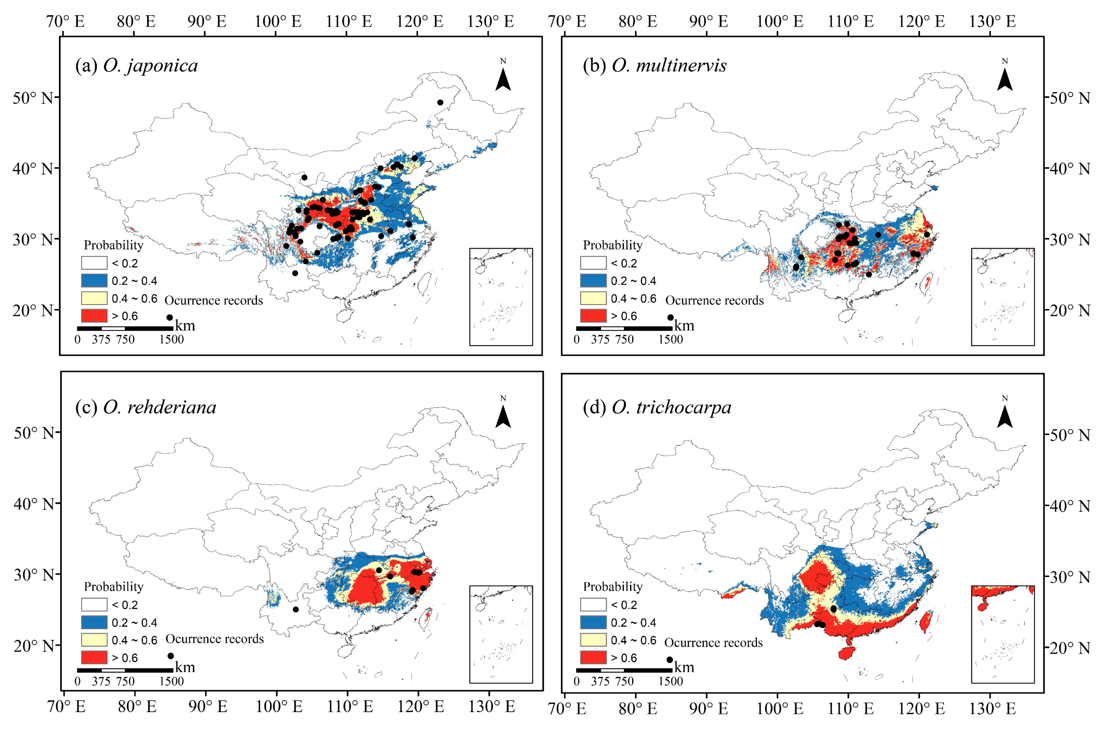
We collected occurrence records of four Ostrya species in China from the Global Biodiversity Information Facility (GBIF, https://www.gbif.org (accessed on 15 June 2020)) [54,55,56], the Chinese Virtual Herbarium (CVH, http://www.cvh.ac.cn (accessed on 15 June 2020)), the Plant Photo Bank of China (PPBC, http://ppbc.iplant.cn (accessed on 15 June 2020)), and the National Specimen Information Infrastructure (NSII, http://www.nsii.org.cn (accessed on 15 June 2020)). We also record the geographic coordinate using a handheld global positioning system (GPS) device according to the field investigation, as well as information in the literature [51,52,57]. Records with unclear or incorrect information were excluded, and the data collected before 1970 were also excluded because they are out of present climatic periods [58]. Each species’ distribution points without duplication in a 2.5 arc-minute resolution grid cell were selected to avoid sample bias and reduce spatial autocorrelation [58,59,60,61], yielding 146 occurrence data points, including 92, 32, 15 and 7 for O. japonica, O. multinervis, O. rehderiana, and O. trichocarpa, respectively (Figure 1).
2.3. Climate Variables
Current climate variables (BIO1-19) were obtained from WorldClim Version 2.1 [62] at 2.5 arc-minute resolution layers of China (Table 1). The 19 bioclimatic layers are the average temperature and precipitation data from 1970 to 2000. Considering that the spatial heterogeneity of climate variability may cause the variation of potential distribution in regional scales, it is necessary to adopt an appropriate climate system model [63,64]. We employed the future climate projections derived from the climate system model in the middle resolution of Beijing Climate Center (BCC-CSM2-MR), demonstrating the best-performing in China with Coupled Model Intercomparison Projects 6 (CIMP6), to forecast the Ostrya distribution in the future [65,66,67]. Additionally, we obtained bioclimatic projections from the model processed for shared socio-economic pathways (SSPs) 1–2.6 and 5–8.5 in the period 2081–2100. SSPs were the new climate projections updated from the representative concentration pathways (RCPs) based on the Sixth Assessment Report (AR6) of the Intergovernmental Panel on Climate Change (IPCC) [65,66]. SSP1-2.6 and SSP5-8.5 represent the low and high radiative forcing by the end of the 21st century, respectively [68,69]. Under SSP1-2.6, the radiative forcing would stabilize at 2.6 W m−2 and global warming would not be increased more than 1.5 °C in 2100, while under SSP5-8.5, emissions would be high enough to produce a radiative forcing of 8.5 W m−2 in 2100 [70].
2.4. Maxent Modeling
We employed Maxent V3.4.1 [40] to predict the potential distributions of Ostrya in current and future scenarios. According to the tutorial of Maxent software [71], environmental layers and occurrence records were tested with each Ostrya species to process the species distribution models. The recommended default values were accepted, including maximum iterations (N = 500), regularization multiplier (N = 1), convergence thresholds (1 × 10⁻⁵), and the maximum number of background points (N = 1 × 10⁵). The background points were taken from the entire study area, which is a priori equally likely to contain the species [72,73,74]. The presence/absence is treated as unknown at these locations, and Maxent contrasts the features at the presence locations to those in the background sample [33]. To reduce the number of correlated variables, the Spearman correlation coefficient and jackknife method were applied to inspect the importance of the climate variables [75,76]. The variable with a higher contribution was rejected when the absolute value of the correlation coefficient of a climate variable pair was higher than 0.8 (p < 0.05). To avoid the over-estimation of models by the area under the receiver operating characteristic curve (AUC), we also evaluated the partial AUC (pAUC) [31,77,78] with R package ntbox [79]. In addition, models running replicated 10 times were required respectively; replicated run type was cross-validation due to the small occurrence data [31,40]. Based on potential distributions in the present scenario, we predicted the range variations of Ostrya in the future. Finally, we analyzed and visualized the occupied areas of Ostrya species in ArcGIS 10.2 (Esri, Redlands, CA, USA). The potential distribution of species was quantified from 0 to 1; we reclassified it into four groups following the method used by Yang et al. [75] and others [80,81,82], namely, least potential (<0.2), moderate potential (0.2–0.4), good potential (0.4–0.6), and high potential (>0.6). Moreover, we calculated the geographic ranges for each of four Ostrya species in the high potential region under present and future climate scenarios.
2.5. Niche Breadth Comparison
The niche breadths of four Ostrya species were estimated by R package ENMTools [83]. B1 and B2, representing the inverse concentration and uncertainty niche breadth respectively, were calculated to quantify the niche breadth of each species, and easily for general use [84]. This index estimated the niche breadth were weighted by the number of different environment variables. The value of 1 indicates generalist taxa that are equally abundant across environments, and 0 indicates specialist taxa that favor specific environment [85]. Each species was calculated with 10 repetitions, the results were compared using one-way ANOVA followed by Tukey’s honestly significant difference (HSD) test. These analyses were performed using R version 4.0.2 [86].
2.6. Niche Overlap Test
To test whether the niches diverge among four Ostrya species, we employed niche equivalency and similarity tests to compare our observed niches overlap against null distributions by R package ecospat [87]. Kernel smoother density was used to estimate the densities of the species occurrence in environmental spaces, while the environmental variables were reduced into axes using principal components analysis to quantify the metrics of niche overlap tests [88].
Schoener’s D and Hellinger’s I were calculated to examine if there were niche overlap between species pairs; they are more robust and direct than other metrics [88]. Metric D reflects microhabitat environments, while I focus on the probability distributions between species pairs [89,90]. To ensure that the null hypothesis can be rejected with high confidence, we performed 1000 randomized pseudo-replicates for each pair of four Ostrya species tested respectively. Both values ranged from 0 (no overlap) to 1 (complete overlap) [87,91]. These analyses were performed using R version 4.0.2 [86].
3. Results
3.1. Model Performance and Contributions of Climate Variables
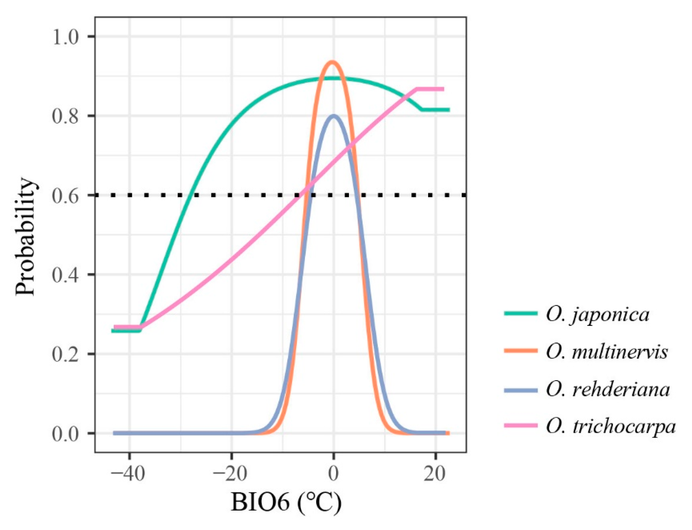
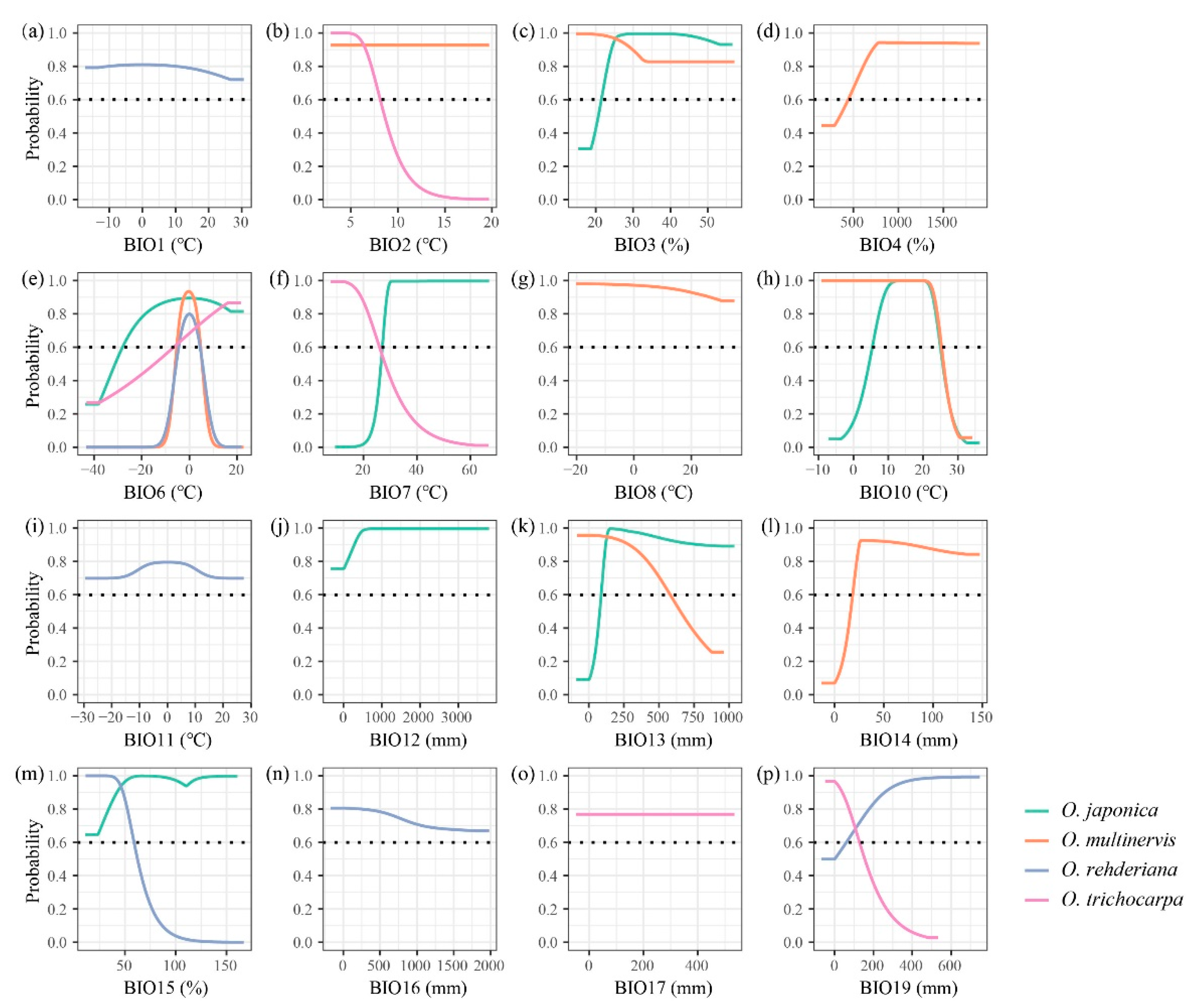
The AUC and pAUC values of all models were higher than 0.8 and 0.9, respectively (Table 2). The distributions of Ostrya species were influenced by different climate variables (Table 1 and Figure A1). The minimum temperature of the coldest month (BIO6) was the principal temperature factor impacting the distributions of four Ostrya species, achieving 59.87% and 70.12% in the contributions of O. rehderiana and O. trichocarpa, respectively. The lowest temperature in winter around ±5 °C was suitable for the growth of O. multinervis and O. rehderiana, while the other two species could adopt a wider range of BIO6 (Figure 2). Besides, Ostrya species were affected by different precipitation variables except for O. trichocarpa which remained mostly unaffected. The distribution of O. multinervis was largely determined by the precipitation of the driest month (BIO14); precipitation in this month lower than 23 mm was unsuitable for O. multinervis (Figure A1l). Precipitation seasonality (BIO15) has an important impact on O. rehderiana, the adaptive range was approximately 62.1% (Figure A1m).
3.2. Potential Distributions of Ostrya under Present and Future Climate Scenarios
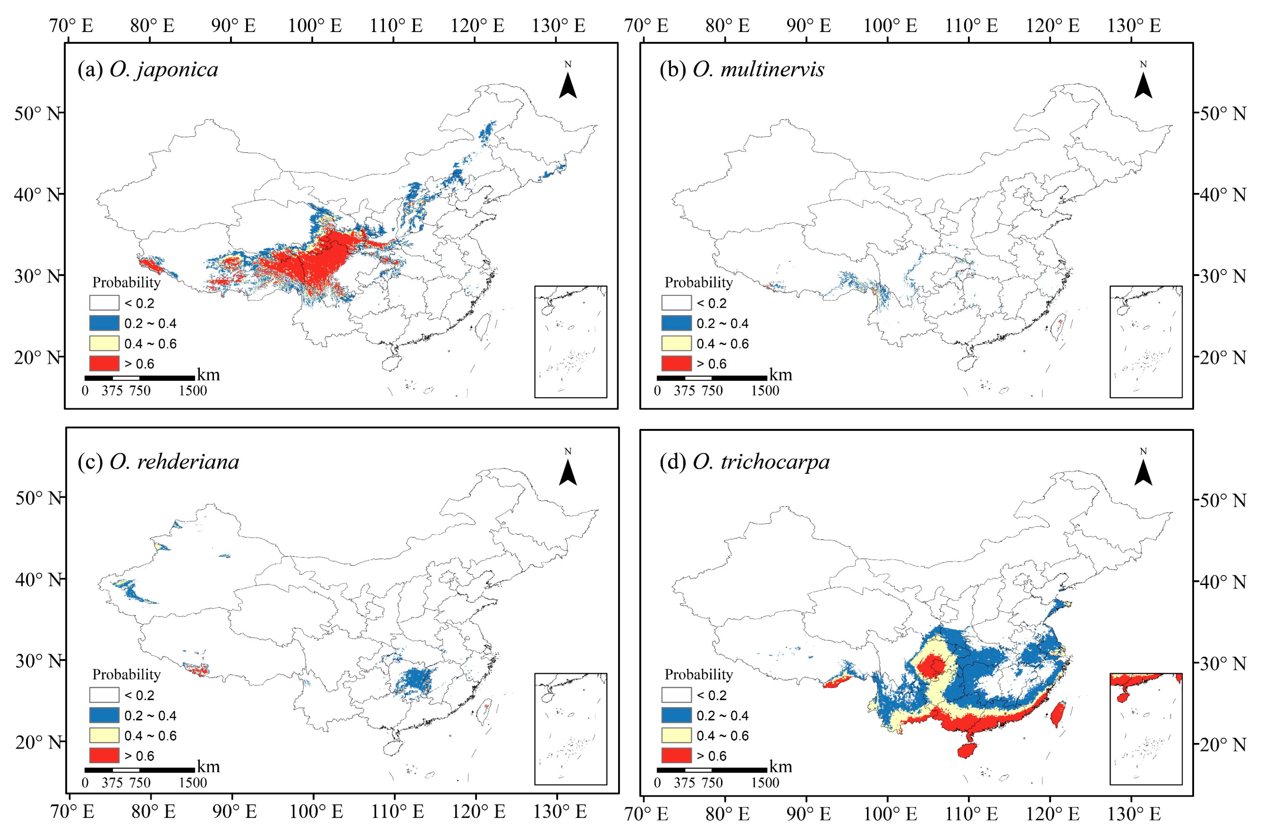
Four Ostrya species showed diverse potential distributions under the present climate scenario (Figure 1). O. japonica, the widest distributed species, was adapted to the climate in the northward and medium-high altitude region. The Loess Plateau was the core distribution region of O. japonica (Figure 1a). O. trichocarpa mainly occurred in the south of China, including Sichuan Basin, southern coastal, Hainan and Taiwan Islands (Figure 1d). O. multinervis exhibited a scattered distribution in the eastern and midwestern China, as well as high-altitude mountains in Taiwan Islands (Figure 1b). Central-eastern China, especially in the Hunan and Zhejiang provinces, was suitable for the growth of O. rehderiana; there was a partial overlapping with O. multinervis in the east (Figure 1b,c).
The climate in the future was more suitable than the present for O. japonica and O. trichocarpa, but the potential distribution range of O. multinervis and O. rehderiana would be reduced significantly in 2081–2100 (Figure 3 and Figure A2). With proceeding climate change, O. japonica and O. trichocarpa were predicted to broaden their potential distribution regions in China. O. japonica expanded the range to higher altitude, including the south Tibetan Plateau and the Hengduan Mountains in the southwest China, the Changbai and Daxinganling Mountains in the northeast China (Figure 3a and Figure A2a). However, under SSP5-8.5, the climate in the northeast China would no longer be suitable for its growth in the end of 21th century (Figure A2a). The high potential distribution ratio of O. japonica would be shifted to 6.07% in 2081–2100 under SSP5-8.5 climate scenario, which was the largest area among all species under SSP5-8.5 (Figure 4b). O. trichocarpa consolidated the core areas of high potential habitat, including Sichuan Basin, southern China, Hainan and Taiwan Islands (Figure 3b and Figure A2b). However, both of O. multinervis and O. rehderiana were confronted with habitat reduction significantly, along with climate change (Figure 3c,d and Figure A2c,d). Although the current distribution was broader, climate change caused the potential habitat of O. multinervis retracting and fragmenting over time (Figure 1b, Figure 3b and Figure A2b). Eastern China would no longer be a suitable shelter for O. rehderiana under SSP5-8.5, where exists the distribution location of this species, as well as with high potential distribution region under the current climate scenario (Figure 1c, Figure 3c and Figure A2c).
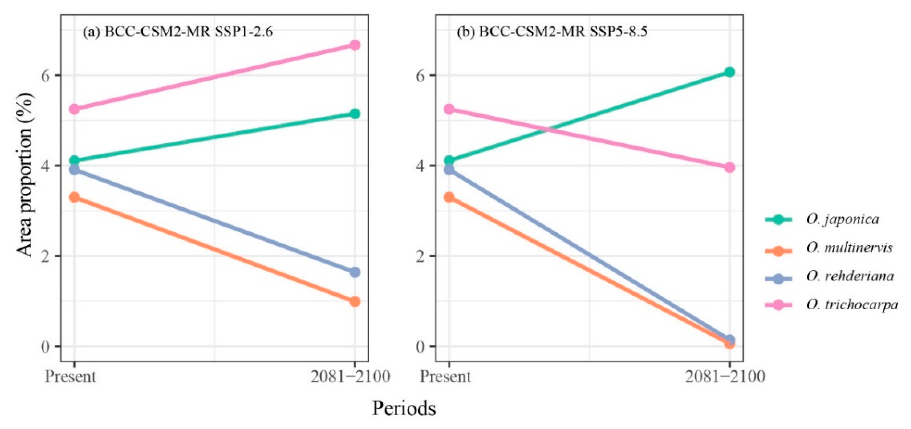
The high potential area shifts between the present and the future scenarios varied among four Ostrya species (Figure 4). The area proportions of O. japonica were increased in both SSPs; O. trichocarpa would expand habitat in SSP1-2.6 while shrinking in SSP5-8.5. O. multinervis and O. rehderiana would dramatically lose their suitable area in SSP1-2.6 and SSP5-8.5 climate scenarios.
3.3. Niche Breadth and Overlap
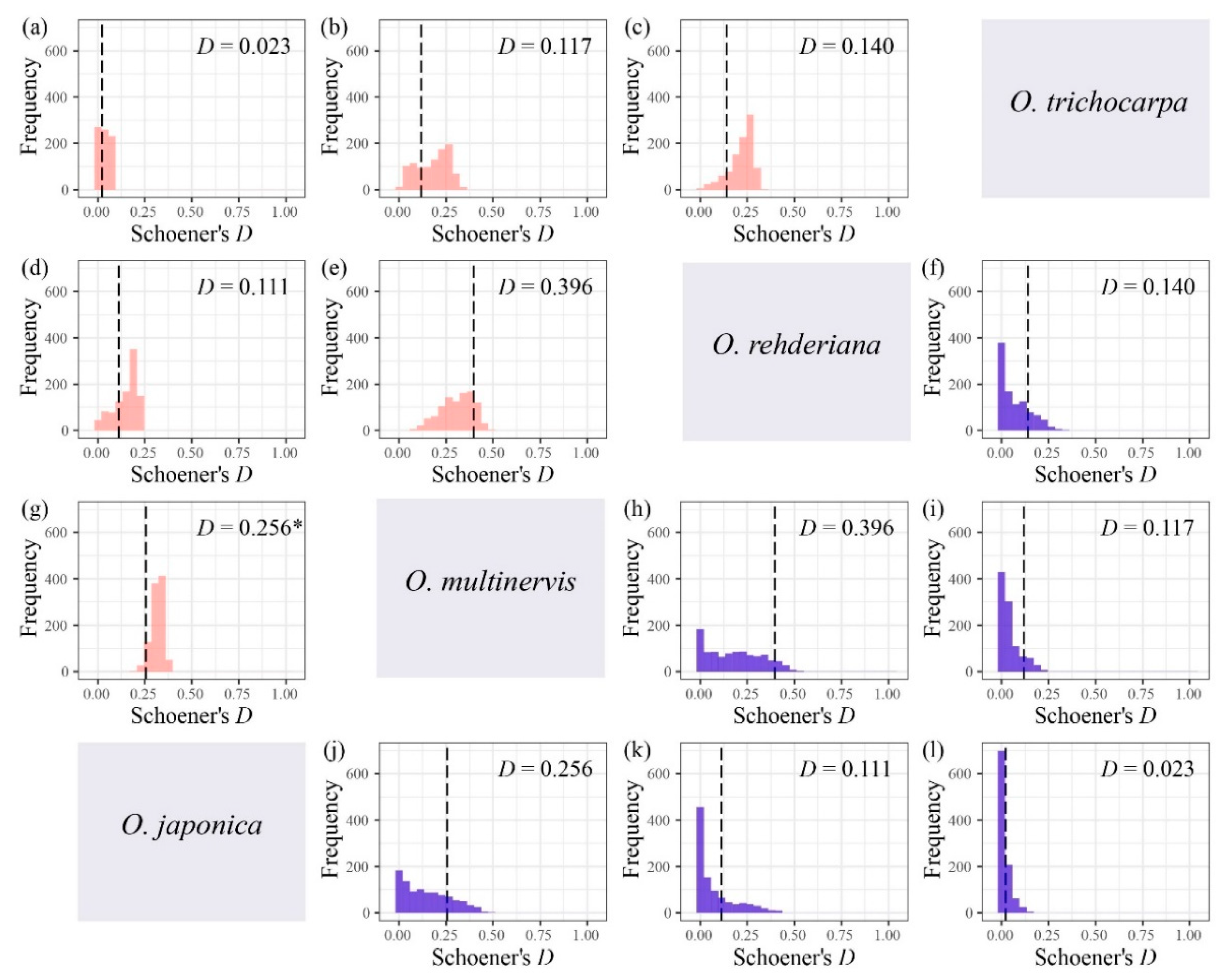
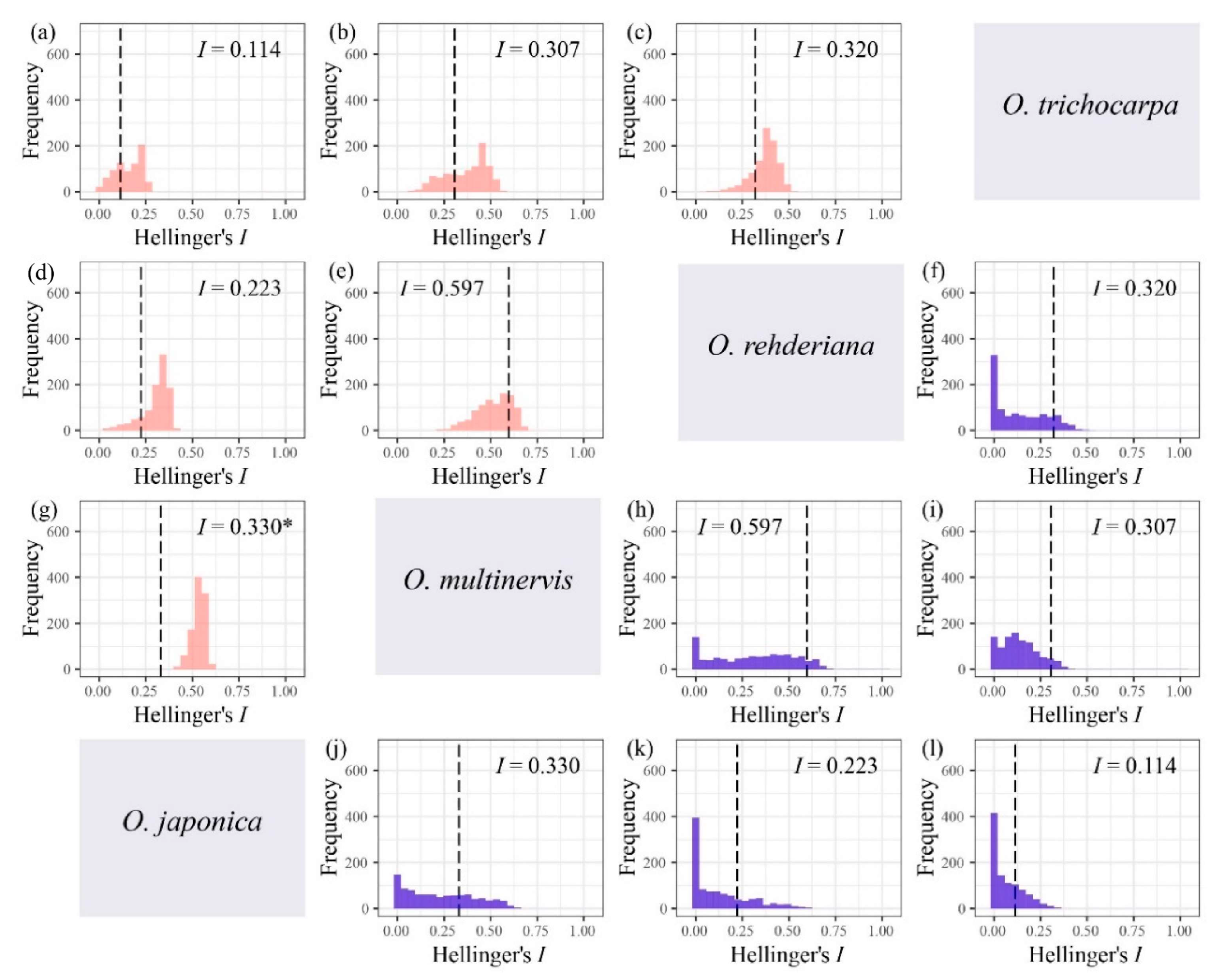
The niche breadth of O. multinervis and O. rehderiana were significantly narrower than O. japonica and O. trichocarpa (Table 3). Either inverse concentration niche breadth B1 or uncertainty niche breadth B2, O. rehderiana and O. multinervis, had similar niche breadth, and both were smaller than those of the other two Ostrya species. Additionally, no niche divergence was observed in four Ostrya species essentially (Figure 5 and Figure A3). Niche overlap existed among species pairs, where Schoener’s D and Hellinger’s I ranged from 0.023 to 0.396 and 0.113 to 0.597, respectively (Figure 5 and Figure A3). The niche overlap of O. multinervis vs. O. rehderiana (D = 0.396, I = 0.597) and O. japonica vs. O. multinervis (D = 0.256, I = 0.330) were greater than other pairs (Figure 5e,h and Figure A3e,h). O. trichocarpa had the least niche overlap with other species, especially for O. japonica (D = 0.023, I = 0.113; Figure 5d and Figure A3d). These measures of overlap to values of overlap were obtained from both the niche equivalency and similarity tests. The null hypothesis in equivalency test for O. japonica vs. O. multinervis (D = 0.256, p = 0.049, (Figure 5g); I = 0.330, p < 0.001, (Figure A3g)) was rejected.
4. Discussion
4.1. Niche Breadth and Distribution Range Size
The niche breadth–range size hypothesis was supported by the results of the four Ostrya species in this study. The models processed by Maxent were creditable in the predicted distributions of Ostrya species in China (Table 2) [77,78]. Two species with broader niche breadth, O. japonica and O. trichocarpa, acquired larger potential geographic occurrence areas and would be further widespread in the future (Table 3 and Figure 3a,d and Figure A2a,d). In contrast, O. multinervis and O. rehderiana with narrower niche breadth had smaller potential geographic occurrence areas and would further narrow the area and have greater extinct possibilities under changed climate in the future (Table 3 and Figure 3b,c and Figure A2b,c). To our knowledge, Ostrya species have not been reported as invasive species, nor as those whose ecological niche shifts appeared fast [90,92], suggesting that niches of the species we studied here would not be able to shift sharply at least in a relatively short period like centuries [93]. In this study with the duration of one hundred years, therefore, the niches of Ostrya species were assumed retained while the geographic ranges are variable in response to climate change [94]. This is also in accordance with previous studies; broad niche species would cross a wider range than species with specialized niche [13,15,16]. Furthermore, no phylogenetic relationship was found in the niche breadth of Ostrya species [51], which was consistent with the study in Fagus species [24].
Our results suggest that climatic variabilities strongly affected the distributions of genus Ostrya in China. Although the niche divergence existed only between O. japonica and O. multinervis, the low niche overlap indicated the variation responded to climatic variables in different species (Figure 5 and Figure A3). Based on the contributions of climate variables (Table 1), the different curves of response to the minimum temperature in the coldest month (BIO6) might be one of the crucial reasons for the divergence of narrow- and wide-ranged Ostrya species. Suitable ranges of the low temperature in winter differed between the narrow- and wide-ranged species (Figure 2), which was the principal bioclimatic variable influencing the distribution of the four Ostrya species. Species with narrow geographic ranges, due to their lower level of genetic variation and plasticity in response to novel selection pressures, tend to be more sensitive to climate change, as compared with those with wide geographic ranges [7,95], just as indicated by Aspinwall et al. [96] that tree species with narrow distribution range are more vulnerable to a warmer climate than widespread ones. The endangerment for O. multinervis and O. rehderiana may be due to their high sensitivity to temperature in winter. O. japonica and O. trichocarpa both having broader potential distribution could withstand lower temperatures (Figure 2). Low temperature range and freezing risk are the major environmental factors determining the distributions of tree species [97,98]. Further research is needed to examine morphological, physiological or molecular responses of Ostrya species to chilling stress. In addition, the temperature in winter would have a significant impact on the naked male inflorescence of Ostrya species [47]. Male inflorescences of O. rehderiana formed from May to June of the previous year and bloomed in April after overwintering [99], while the germination of seeds in O. rehderiana needs prolonging (>100 d) cold stratification to break dormancy [100]. The narrow winter temperature range requirement of O. rehderiana appears to be an adaptability compromise between these factors (Figure 2). On the other hand, O. multinervis and O. rehderiana were more sensitive to precipitation than the other two species, especially in the driest month and seasonality during one year (Table 1 and Figure A1l,m). The increasing unbalanced and extreme precipitation under future climate scenarios might be another issue that determines the divergence of range sizes with broader niche species [101].
Notably, the niche breadth of least-record species O. trichocarpa was wider than other narrow-ranged species (O. multinervis and O. rehderiana), and it also had larger potential habitats in the present and future. The ecological niche of species contains two dimensions of both fundamental and realized one [102,103]. The former involves the relationship between species and environmental factors, while the latter considers biological interactions [103,104,105,106]. Our results modeled the fundamental niche of Ostrya species only, while the effects of intra- or inter-specific relationships were not considered. Moreover, the existence of plants also depends on various environmental conditions, the climate niche that we focus on is one type of fundamental niche [107]. This may be one of the reasons for the difference between O. trichocarpa and the other two narrowly distributed species. More studies on those species are needed in the future. Besides, the discrepancy might be attributed to the accuracy of modeling. It is undeniable that the model’s accuracy was positively related to the sample size [108,109], even though Maxent could achieve excellent performance on predicting the distribution of narrow ranged species [110]. The extremely small sample size of O. trichocarpa and presence-only data used in models might increase the uncertainty of Maxent model outputs [39,111]. More algorithms should be considered to improve the accuracy of modeling [112]; reciprocal transplantation experiments also should be needed to test the performance of models [113,114,115].
4.2. Conservation Implications
Most of the narrow-ranged species are rare species and at high risk of extinction [26,116,117]. The positive relationships between range size and niche breadth could provide a reliable reference for conservation planning and policy making. Our findings of potential Ostrya suitable habitats in current and future climate scenarios are suggestive for their conservation.
The SDMs projected a dramatic reduction in the distribution areas of O. multinervis and O. rehderiana, where the survival probability in east China would be reduced. O. rehderiana would have a high risk of extinction despite its potential distribution region in Zhejiang, Hunan and Jiangxi Provinces. O. trichocarpa would expand enormously in the future; its potential habitat would range from the southern coastal areas to the inland areas of southwestern China as well as Taiwan and Hainan Islands (Figure 3 and Figure A2). Climate change would intensify habitat fragmentation of O. multinervis and further human activities would aggravate the process, if possible, which would increase the difficulty of their conservation (Figure 3b and Figure A2b) [26,118,119,120]. Considering of the distribution region shift of O. rehderiana, ex situ conservation or national nature reserves in other places such as Hunan Province should be implemented (Figure 1c and Figure 3c) [115]. Considering that deleterious mutations accumulated so far are one of the causes for the rarity of O. rehderiana, the genetic diversity should be maintained through conserving Ostrya [52].
4.3. Limitations
In this study, the niche breathes of Ostrya were estimated by a model whose performance would be limited by the dimensionality of predictive factors [113,121]. For example, the species with samara (e.g., Ostrya species) rely on wind dispersal [47,122], while the seedlings of O. rehderiana are weak and easy damage, for instance by strong wind [99]. The topographic heterogeneity in soil nutrients and microclimate would have an impact on the species diversity [123,124]. The opposite responses to human influence might aggravate the differences between rare and widespread species [26,44]. Thus, future studies should consider more possible influence factors on the model construction. Unfortunately, there have been very few detailed demonstrations on other abiotic and biotic environmental factors which may vary in the future, causing our results to deviate from the actual situation [125,126]. Furthermore, the model’s accuracy is usually positively related to the sample size as mentioned in 4.1 [108,109]. Limited by data availability, the occurrence records included in our study were not large enough. Thus, more field surveys would be needed to extend the knowledge about the distributions of Ostrya species in China [58,76]. Field studies, including common garden and reciprocal transplantation experiments, should also be taken to further compare widespread and rare species under environmental tolerance [113,114].
Moreover, genetic variation has an impact on the distribution of species, and the accumulation of deleterious mutations might explain why O. rehderiana is rare [52]. Widespread species O. japonica has higher genetic diversity than others [57]. The species diversification rate is also driven by the climate change [127]. Thus, more attention should be paid to the genetic diversity impacting on species niche studies in the future.
5. Conclusions
Potential distribution range sizes of the four Ostrya species would positively correlate with their niche breadth in the present and future scenarios; niche breadth would determine the distribution variations with climate change. The lowest temperature in winter would be the major climatic factor influencing the establishments of the four Ostrya species. The wide niche breadth species (O. japonica and O. trichocarpa) would be further widespread in the future scenarios while narrowly distributed species (O. multinervis and O. rehderiana) having narrower niche currently would further narrow their distribution range under changing climate and might be subjected to a high risk of extinction in future scenarios. Our findings support the niche breadth–range size hypothesis and provide a valuable reference for the conservation of endangered and rare species like O. rehderiana. In the future, research topics related to range sizes of more taxa on broad biogeographic scales and their dynamics in a changing climate are expected.
Author Contributions
Conceptualization, Y.-B.S. and M.D.; methodology, S.-L.T.; software, S.-L.T.; validation, S.-L.T.; formal analysis, S.-L.T.; investigation, S.-L.T.; resources, S.-L.T., Y.-B.S., B.Z. and M.D.; data curation, S.-L.T.; writing—original draft preparation, S.-L.T., Y.-B.S., B.Z. and M.D.; writing—review and editing, S.-L.T., Y.-B.S., B.Z. and M.D.; visualization, S.-L.T., Y.-B.S. and M.D.; supervision, M.D.; project administration, M.D.; funding acquisition, B.Z. and M.D. All authors have read and agreed to the published version of the manuscript.
Funding
This research was funded by the National Key Research and Development Program of China, grant numbers 2016YFC0503100, 2017YFC0505301; and the National Natural Science Foundation of China, grant number 31670429.
Institutional Review Board Statement
Not applicable.
Informed Consent Statement
Not applicable.
Data Availability Statement
The data presented in this study are available on request from the corresponding author.
Acknowledgments
We thank Wei-Jun Zhang for his help in data collection.
Conflicts of Interest
The authors declare no conflict of interest.
Appendix A
Figure A1.
Response curves of four Ostrya species, i.e., O. japonica, O. multinervis, O. rehderiana, and O. trichocarpa, presence probability affected by climate variables, i.e., BIO1 (a), BIO2 (b), BIO3 (c), BIO4 (d), BIO6 (e), BIO7 (f), BIO8 (g), BIO10 (h), BIO11 (i), BIO12 (j), BIO13 (k), BIO14 (l), BIO15 (m), BIO16 (n), BIO17 (o), and BIO19 (p). See Table 2 for the meaning of each climatic variable. The black dotted line represents that the probability of species existing is 0.6, species would archive high potential adaptation above this line.

Figure A2.
Potential habitats of four Ostrya species, i.e., O. japonica (a), O. multinervis (b), O. rehderiana (c), and O. trichocarpa (d), under the climate scenario BCC-CSM2-MR SSP5-8.5 in the period 2081–2100. The values for species occurrence probability ranged between 0 and 1, i.e., least potential (<0.2), moderate potential (0.2–0.4), good potential (0.4–0.6), and high potential (>0.6).

Figure A3.
Niche overlap tests for four Ostrya species based on Hellinger’s I, i.e., O. japonica vs. O. trichocarpa (a), O. multinervis vs. O. trichocarpa (b), O. rehderiana vs. O. trichocarpa (c), O. japonica vs. O. rehderiana (d), O. multinervis vs. O. rehderiana (e), and O. japonica vs. O. multinervis (g) using niche equivalency test; O. rehderiana vs. O. trichocarpa (f), O. multinervis vs. O. rehderiana (h), O. multinervis vs. O. trichocarpa (i), O. japonica vs. O. multinervis (j), O. japonica vs. O. rehderiana (k), and O. japonica vs. O. trichocarpa (l) using similarity test. Pink and blue represent equivalency and similarity tests respectively. The Matric I assumed the niche overlap in distribution probability (Warren et al., 2008), ranging from 0 (no overlap) to 1 (complete overlap). The black dotted line represents the observed niche overlap between species pair (i.e., the empirical values of I), whereas the histograms are those expected under the null hypotheses, and * represents the niches are significantly (p < 0.05) more different than expected by random.

References
- Schwartz, M.W.; Iverson, L.R.; Prasad, A.M.; Matthews, S.N.; O’Connor, R.J. Predicting extinctions as a result of climate change. Ecology 2006, 87, 1611–1615. [Google Scholar] [CrossRef]
- Hayes, K.R.; Barry, S.C. Are there any consistent predictors of invasion success? Biol. Invasions 2008, 10, 483–506. [Google Scholar] [CrossRef]
- Stevens, G.C. The latitudinal gradient in geographical range: How so many species coexist in the tropics. Am. Nat. 1989, 133, 240–256. [Google Scholar] [CrossRef]
- Brown, J.H.; Stevens, G.C.; Kaufman, D.M. The geographic range: Size, shape, boundaries, and internal structure. Annu. Rev. Ecol. Evol. Syst. 1996, 27, 597–623. [Google Scholar] [CrossRef] [Green Version]
- Gaston, K.J. Species-range-size distributions: Patterns, mechanisms and implications. Trends Ecol. Evol. 1996, 11, 197–201. [Google Scholar] [CrossRef]
- Lester, S.E.; Ruttenberg, B.I.; Gaines, S.D.; Kinlan, B.P. The relationship between dispersal ability and geographic range size. Ecol. Lett. 2007, 10, 745–758. [Google Scholar] [CrossRef] [PubMed]
- Sheth, S.N.; Angert, A.L. The evolution of environmental tolerance and range size: A comparison of geographically restricted and widespread. Mimulus. Evol. 2014, 68, 2917–2931. [Google Scholar] [CrossRef] [PubMed]
- Colwell, R.K.; Hurtt, G.C. Nonbiological gradients in species richness and a spurious Rapoport effect. Am. Nat. 1994, 144, 570–595. [Google Scholar] [CrossRef]
- Ohlemüller, R.; Anderson, B.J.; Araujo, M.B.; Butchart, S.H.; Kudrna, O.; Ridgely, R.S.; Thomas, C.D. The coincidence of climatic and species rarity: High risk to small-range species from climate change. Biol. Lett. 2008, 4, 568–572. [Google Scholar] [CrossRef] [PubMed] [Green Version]
- Brown, J.H. On the relationship between abundance and distribution of species. Am. Nat. 1984, 124, 255–279. [Google Scholar] [CrossRef]
- Gaston, K.J.; Spicer, J.I. The relationship between range size and niche breadth: A test using five species of Gammarus (Amphipoda). Glob. Ecol. Biogeogr. 2001, 10, 179–188. [Google Scholar] [CrossRef]
- Boulangeat, I.; Lavergne, S.; van Es, J.; Garraud, L.; Thuiller, W. Niche breadth, rarity and ecological characteristics within a regional flora spanning large environmental gradients. J. Biogeogr. 2012, 39, 204–214. [Google Scholar] [CrossRef]
- Botts, E.A.; Erasmus, B.F.N.; Alexander, G.J.; Lawlor, J. Small range size and narrow niche breadth predict range contractions in South African frogs. Glob. Ecol. Biogeogr. 2013, 22, 567–576. [Google Scholar] [CrossRef]
- Carrillo-Angeles, I.G.; Suzán-Azpiri, H.; Mandujano, M.C.; Golubov, J.; Martínez-Ávalos, J.G. Niche breadth and the implications of climate change in the conservation of the genus Astrophytum (Cactaceae). J. Arid Environ. 2016, 124, 310–317. [Google Scholar] [CrossRef]
- Yu, F.; Groen, T.A.; Wang, T.; Skidmore, A.K.; Huang, J.; Ma, K. Climatic niche breadth can explain variation in geographical range size of alpine and subalpine plants. Int. J. Geogr. Inf. Sci. 2016, 31, 190–212. [Google Scholar] [CrossRef] [Green Version]
- Vincent, H.; Bornand, C.N.; Kempel, A.; Fischer, M. Rare species perform worse than widespread species under changed climate. Biol. Invasions 2020, 246. [Google Scholar] [CrossRef]
- Lynch, M.; Gabriel, W. Environmental tolerance. Am. Nat. 1987, 129, 283–303. [Google Scholar] [CrossRef] [Green Version]
- Bolnick, D.I.; Svanbäck, R.; Fordyce, J.A.; Yang, L.H.; Davis, J.M.; Hulsey, C.D.; Forister, M.L. The ecology of individuals: Incidence and implications of individual specialization. Am. Nat. 2003, 161, 1–28. [Google Scholar] [CrossRef]
- Schwilk, D.W.; Ackerly, D.D. Limiting similarity and functional diversity along environmental gradients. Ecol. Lett. 2005, 8, 272–281. [Google Scholar] [CrossRef]
- Siqueira, T.; Bini, L.M.; Roque, F.O.; Marques Couceiro, S.R.; Trivinho-Strixino, S.; Cottenie, K. Common and rare species respond to similar niche processes in macroinvertebrate metacommunities. Ecography 2012, 35, 183–192. [Google Scholar] [CrossRef]
- Carscadden, K.A.; Emery, N.C.; Arnillas, C.A.; Cadotte, M.W.; Afkhami, M.E.; Gravel, D.; Livingstone, S.W.; Wiens, J.J. Niche breadth: Causes and consequences for ecology, evolution, and conservation. Quart. Rev. Biol. 2020, 95, 179–214. [Google Scholar] [CrossRef]
- Slatyer, R.A.; Hirst, M.; Sexton, J.P. Niche breadth predicts geographical range size: A general ecological pattern. Ecol. Lett. 2013, 16, 1104–1114. [Google Scholar] [CrossRef] [PubMed]
- Hirst, M.J.; Griffin, P.C.; Sexton, J.P.; Hoffmann, A.A. Testing the niche-breadth–range-size hypothesis: Habitat specialization vs. performance in Australian alpine daisies. Ecology 2017, 98, 2708–2724. [Google Scholar] [CrossRef] [PubMed]
- Cai, Q.; Welk, E.; Ji, C.; Fang, W.; Sabatini, F.M.; Zhu, J.; Zhu, J.; Tang, Z.; Attorre, F.; Campos, J.A.; et al. The relationship between niche breadth and range size of beech (Fagus) species worldwide. J. Biogeogr. 2021, 48, 1240–1253. [Google Scholar] [CrossRef]
- Gaston, K.J.; Fuller, R.A. The sizes of species’ geographic ranges. J. Appl. Ecol. 2009, 46, 1–9. [Google Scholar] [CrossRef]
- Xu, W.B.; Svenning, J.C.; Chen, G.K.; Zhang, M.G.; Huang, J.H.; Chen, B.; Ordonez, A.; Ma, K.P. Human activities have opposing effects on distributions of narrow-ranged and widespread plant species in China. Proc. Natl. Acad. Sci. USA 2019, 116, 26674–26681. [Google Scholar] [CrossRef] [Green Version]
- Gaston, K.J. Species-range size distributions: Products of speciation, extinction and transformation. Philos. Trans. R. Soc. B 1998, 353, 219–230. [Google Scholar] [CrossRef] [Green Version]
- Purvis, A.; Gittleman, J.L.; Cowlishaw, G.; Mace, G.M. Predicting extinction risk in declining species. Proc. R. Soc. B. Biol. Sci. 2000, 267, 1947–1952. [Google Scholar] [CrossRef] [Green Version]
- Wan, J.Z.; Wang, C.J.; Yu, F.H. Spatial conservation prioritization for dominant tree species of Chinese forest communities under climate change. Clim. Chang. 2017, 144, 303–316. [Google Scholar] [CrossRef]
- Elith, J.; Leathwick, J.R. Species distribution models: Ecological explanation and prediction across space and time. Annu. Rev. Ecol. Evol. Syst. 2009, 40, 677–697. [Google Scholar] [CrossRef]
- Zurell, D.; Franklin, J.; König, C.; Bouchet, P.J.; Dormann, C.F.; Elith, J.; Fandos, G.; Feng, X.; Guillera-Arroita, G.; Guisan, A.; et al. A standard protocol for reporting species distribution models. Ecography 2020, 43, 1261–1277. [Google Scholar] [CrossRef]
- Franklin, J. Species distribution models in conservation biogeography: Developments and challenges. Divers. Distrib. 2013, 19, 1217–1223. [Google Scholar] [CrossRef]
- Merow, C.; Smith, M.J.; Silander, J.A. A practical guide to MaxEnt for modeling species’ distributions: What it does, and why inputs and settings matter. Ecography 2013, 36, 1058–1069. [Google Scholar] [CrossRef]
- He, Q.; Zhao, R.; Zhu, Z. Geographical distribution simulation and comparative analysis of Carpinus viminea and C. londoniana. Glob. Ecol. Conserv. 2020, 21, e00825. [Google Scholar] [CrossRef]
- Elith, J.; Graham, C.H. Do they? How do they? Why do they differ? On finding reasons for differing performances of species distribution models. Ecography 2009, 32, 66–77. [Google Scholar] [CrossRef]
- Pearson, R.G.; Raxworthy, C.J.; Nakamura, M.; Peterson, A.T. Predicting species distributions from small numbers of occurrence records: A test case using cryptic geckos in Madagascar. J. Biogeogr. 2006, 34, 102–117. [Google Scholar] [CrossRef]
- Tsoar, A.; Allouche, O.; Steinitz, O.; Rotem, D.; Kadmon, R. A comparative evaluation of presence-only methods for modelling species distribution. Divers. Distrib. 2007, 13, 397–405. [Google Scholar] [CrossRef]
- Kaky, E.; Nolan, V.; Alatawi, A.; Gilbert, F. A comparison between Ensemble and MaxEnt species distribution modelling approaches for conservation: A case study with Egyptian medicinal plants. Ecol. Inform. 2020, 60, 101150. [Google Scholar] [CrossRef]
- Elith, J.; Phillips, S.J.; Hastie, T.; Dudik, M.; Chee, Y.E.; Yates, C.J. A statistical explanation of MaxEnt for ecologists. Divers. Distrib. 2011, 17, 43–57. [Google Scholar] [CrossRef]
- Phillips, S.J.; Anderson, R.P.; Dudík, M.; Schapire, R.E.; Blair, M.E. Opening the black box: An open-source release of Maxent. Ecography 2017, 40, 887–893. [Google Scholar] [CrossRef]
- Rhoden, C.M.; Peterman, W.E.; Taylor, C.A. Maxent-directed field surveys identify new populations of narrowly endemic habitat specialists. PeerJ 2017, 5, e3632. [Google Scholar] [CrossRef] [Green Version]
- Zhao, R.; Chu, X.; He, Q.; Tang, Y.; Song, M.; Zhu, Z. Modeling current and future potential geographical distribution of Carpinus tientaiensis, a critically endangered species from China. Forests 2020, 11, 774. [Google Scholar] [CrossRef]
- Visger, C.J.; Germain-Aubrey, C.C.; Patel, M.; Sessa, E.B.; Soltis, P.S.; Soltis, D.E. Niche divergence between diploid and autotetraploid Tolmiea. Am. J. Bot. 2016, 103, 1396–1406. [Google Scholar] [CrossRef] [Green Version]
- Yu, F.; Wang, T.; Groen, T.A.; Skidmore, A.K.; Yang, X.; Ma, K.; Wu, Z. Climate and land use changes will degrade the distribution of Rhododendrons in China. Sci. Total. Environ. 2019, 659, 515–528. [Google Scholar] [CrossRef]
- Bozkurt, A.; Erdin, N. Wood Material Technology Handbook; Istanbul University Publication, Faculty of Forestry Publication: Istanbul, Turkey, 1997. [Google Scholar]
- Korkut, S.; Guller, B. Physical and mechanical properties of European Hophornbeam (Ostrya carpinifolia Scop.) wood. Bioresour. Technol. 2008, 99, 4780–4785. [Google Scholar] [CrossRef] [PubMed]
- Chen, Z.D.; Manchester, S.R.; Sun, H.Y. Phylogeny and evolution of the Betulaceae as inferred from DNA sequences, morphology, and paleobotany. Am. J. Bot. 1999, 86, 1168–1181. [Google Scholar] [CrossRef] [PubMed]
- Holstein, N.; Weigend, M. No taxon left behind?—A critical taxonomic checklist of Carpinus and Ostrya (Coryloideae, Betulaceae). Eur. J. Taxon. 2017, 375, 1–52. [Google Scholar] [CrossRef] [Green Version]
- Fang, Z.; Zhao, S.; Skvortsov, A. Flora of China. Harv. Pap. Bot. 1999, 4, 300–301. [Google Scholar]
- Shaw, K.; Roy, S.; Wilson, B. The IUCN Red List of Threatened Species; IUCN: Gland, Switzerland, 2014. [Google Scholar] [CrossRef]
- Lu, Z.; Zhang, D.; Liu, S.; Yang, X.; Liu, X.; Liu, J. Species delimitation of Chinese hop-hornbeams based on molecular and morphological evidence. Ecol. Evol. 2016, 6, 4731–4740. [Google Scholar] [CrossRef] [Green Version]
- Yang, Y.; Ma, T.; Wang, Z.; Lu, Z.; Li, Y.; Fu, C.; Chen, X.; Zhao, M.; Olson, M.S.; Liu, J. Genomic effects of population collapse in a critically endangered ironwood tree Ostrya rehderiana. Nat. Commun. 2018, 9, 5449. [Google Scholar] [CrossRef]
- National Forestry and Grassland Administration, National Key Protected Wild Plant List. Available online: https://www.forestry.gov.cn/main/153/20200710/085720879652689.html (accessed on 9 July 2020).
- GBIF.org. Occurrence Download (Ostrya multinervis). Available online: https://doi.org/10.15468/dl.5a4xx3 (accessed on 15 June 2020).
- GBIF.org. Occurrence Download (Ostrya rehderiana). Available online: https://doi.org/10.15468/dl.accazd (accessed on 15 June 2020).
- GBIF.org. Occurrence Download (Ostrya japonica). Available online: https://doi.org/10.15468/dl.rr9ytq (accessed on 15 June 2020).
- Jiang, Y.; Yang, Y.; Lu, Z.; Wan, D.; Ren, G. Interspecific delimitation and relationships among four Ostrya species based on plastomes. BMC Genet. 2019, 20, 33. [Google Scholar] [CrossRef] [Green Version]
- Dyderski, M.K.; Paź, S.; Frelich, L.E.; Jagodziński, A.M. How much does climate change threaten European forest tree species distributions? Glob. Chang. Biol. 2018, 24, 1150–1163. [Google Scholar] [CrossRef] [PubMed]
- Boria, R.A.; Olson, L.E.; Goodman, S.M.; Anderson, R.P. Spatial filtering to reduce sampling bias can improve the performance of ecological niche models. Ecol. Model. 2014, 275, 73–77. [Google Scholar] [CrossRef]
- Fortin, M.J. Effects of sampling unit resolution on the estimation of spatial autocorrelation. Ecoscience 2016, 6, 636–641. [Google Scholar] [CrossRef]
- Moore, T.E.; Bagchi, R.; Aiello-Lammens, M.E.; Schlichting, C.D. Spatial autocorrelation inflates niche breadth–range size relationships. Glob. Ecol. Biogeogr. 2018, 27, 1426–1436. [Google Scholar] [CrossRef]
- Fick, S.E.; Hijmans, R.J. WorldClim 2: New 1-km spatial resolution climate surfaces for global land areas. Int. J. Climatol. 2017, 37, 4302–4315. [Google Scholar] [CrossRef]
- Ashcroft, M.B.; Chisholm, L.A.; French, K.O. Climate change at the landscape scale: Predicting fine-grained spatial heterogeneity in warming and potential refugia for vegetation. Glob. Chang. Biol. 2009, 15, 656–667. [Google Scholar] [CrossRef] [Green Version]
- Dobrowski, S.Z. A climatic basis for microrefugia: The influence of terrain on climate. Glob. Chang. Biol. 2011, 17, 1022–1035. [Google Scholar] [CrossRef]
- Wu, T.; Lu, Y.; Fang, Y.; Xin, X.; Li, L.; Li, W.; Jie, W.; Zhang, J.; Liu, Y.; Zhang, L.; et al. The Beijing climate center climate system model (BCC-CSM): The main progress from CMIP5 to CMIP6. Geosci. Model. Dev. 2019, 12, 1573–1600. [Google Scholar] [CrossRef] [Green Version]
- Wu, T.W.; Song, L.C.; Li, W.P.; Wang, Z.Z.; Zhang, H.; Xin, X.G.; Zhang, Y.W.; Zhang, L.; Li, J.L.; Wu, F.H.; et al. An overview of BCC climate system model development and application for climate change studies. J. Meteorol. Res. 2014, 28, 34–56. [Google Scholar] [CrossRef]
- Xin, X.; Wu, T.; Li, J.; Wang, Z.; Li, W.; Wu, F. How well does BCC_CSM1. 1 reproduce the 20th century climate change over China? Atmos. Sci. Lett. 2013, 6, 21–26. [Google Scholar] [CrossRef] [Green Version]
- O’Neill, B.C.; Tebaldi, C.; van Vuuren, D.P.; Eyring, V.; Friedlingstein, P.; Hurtt, G.; Knutti, R.; Kriegler, E.; Lamarque, J.F.; Lowe, J.; et al. The scenario model intercomparison project (ScenarioMIP) for CMIP6. Geosci. Model. Dev. 2016, 9, 3461–3482. [Google Scholar] [CrossRef] [Green Version]
- Riahi, K.; van Vuuren, D.P.; Kriegler, E.; Edmonds, J.; O’Neill, B.C.; Fujimori, S.; Bauer, N.; Calvin, K.; Dellink, R.; Fricko, O.; et al. The shared socioeconomic pathways and their energy, land use, and greenhouse gas emissions implications: An overview. Glob. Environ. Chang. 2017, 42, 153–168. [Google Scholar] [CrossRef] [Green Version]
- Van Vuuren, D.P.; Kriegler, E.; O’Neill, B.C.; Ebi, K.L.; Riahi, K.; Carter, T.R.; Edmonds, J.; Hallegatte, S.; Kram, T.; Mathur, R. A new scenario framework for climate change research: Scenario matrix architecture. Clim. Chang. 2014, 122, 373–386. [Google Scholar] [CrossRef] [Green Version]
- Phillips, S.J. A brief tutorial on Maxent. AT&T Res. 2005, 190, 231–259. [Google Scholar]
- Phillips, S.J.; Dudik, M. Modeling of species distributions with Maxent: New extensions and a comprehensive evaluation. Ecography 2008, 31, 161–175. [Google Scholar] [CrossRef]
- VanDerWal, J.; Shoo, L.P.; Graham, C.; Williams, S.E. Selecting pseudo-absence data for presence-only distribution modeling: How far should you stray from what you know? Ecol. Model. 2009, 220, 589–594. [Google Scholar] [CrossRef]
- Elith, J.; Kearney, M.; Phillips, S. The art of modelling range-shifting species. Methods Ecol. Evol. 2010, 1, 330–342. [Google Scholar] [CrossRef]
- Yang, X.Q.; Kushwaha, S.P.S.; Saran, S.; Xu, J.; Roy, P.S. Maxent modeling for predicting the potential distribution of medicinal plant, Justicia adhatoda L. in Lesser Himalayan foothills. Ecol. Eng. 2013, 51, 83–87. [Google Scholar] [CrossRef]
- Puchałka, R.; Dyderski, M.K.; Vítková, M.; Sádlo, J.; Klisz, M.; Netsvetov, M.; Prokopuk, Y.; Matisons, R.; Mionskowski, M.; Wojda, T.; et al. Black locust (Robinia pseudoacacia L.) range contraction and expansion in Europe under changing climate. Glob. Chang. Biol. 2021, 27, 1587–1600. [Google Scholar] [CrossRef]
- Fielding, A.H.; Bell, J.F. A review of methods for the assessment of prediction errors in conservation presence/absence models. Environ. Conserv. 1997, 24, 38–49. [Google Scholar] [CrossRef]
- Slater, H.; Michael, E. Predicting the current and future potential distributions of Lymphatic filariasis in Africa using Maximum Entropy Ecological Niche Modelling. PLoS ONE 2012, 7, e32202. [Google Scholar] [CrossRef]
- Osorio-Olvera, L.; Lira-Noriega, A.; Soberón, J.; Peterson, A.T.; Falconi, M.; Contreras-Díaz, R.G.; Martínez-Meyer, E.; Barve, V.; Barve, N. ntbox: An r package with graphical user interface for modelling and evaluating multidimensional ecological niches. Methods Ecol. Evol. 2020, 11, 1199–1206. [Google Scholar] [CrossRef]
- Abolmaali, S.M.R.; Tarkesh, M.; Bashari, H. MaxEnt modeling for predicting suitable habitats and identifying the effects of climate change on a threatened species, Daphne mucronata, in central Iran. Ecol. Inform. 2018, 43, 116–123. [Google Scholar] [CrossRef]
- Gebrewahid, Y.; Abrehe, S.; Meresa, E.; Eyasu, G.; Abay, K.; Gebreab, G.; Kidanemariam, K.; Adissu, G.; Abreha, G.; Darcha, G. Current and future predicting potential areas of Oxytenanthera abyssinica (A. Richard) using MaxEnt model under climate change in Northern Ethiopia. Ecol. Process. 2020, 9, 6. [Google Scholar] [CrossRef] [Green Version]
- Salvà-Catarineu, M.; Romo, A.; Mazur, M.; Zielińska, M.; Minissale, P.; Dönmez, A.A.; Boratyńska, K.; Boratyński, A. Past, present, and future geographic range of the relict Mediterranean and Macaronesian Juniperus phoenicea complex. Ecol. Evol. 2021, 11, 5075–5095. [Google Scholar] [CrossRef] [PubMed]
- Warren, D.L.; Matzke, N.J.; Cardillo, M.; Baumgartner, J.B.; Beaumont, L.J.; Turelli, M.; Glor, R.E.; Huron, N.A.; Simões, M.; Iglesias, T.L.; et al. ENMTools 1.0: An R package for comparative ecological biogeography. Ecography 2021, 44, 504–511. [Google Scholar] [CrossRef]
- Feinsinger, P.; Spears, E.E.; Poole, R.W. A simple measure of niche breadth. Ecology 1981, 62, 27–32. [Google Scholar] [CrossRef]
- Levins, R. Evolution in Changing Environments: Some Theoretical Explorations; Princeton University Press: Princeton, NJ, USA, 1968. [Google Scholar]
- R Core Team. R: A Language and Environment for Statistical Computing; R Foundation for Statistical Computing: Vienna, Austria, 2020. [Google Scholar]
- Di Cola, V.; Broennimann, O.; Petitpierre, B.; Breiner, F.T.; D’Amen, M.; Randin, C.; Engler, R.; Pottier, J.; Pio, D.; Dubuis, A.; et al. ecospat: An R package to support spatial analyses and modeling of species niches and distributions. Ecography 2017, 40, 774–787. [Google Scholar] [CrossRef]
- Broennimann, O.; Fitzpatrick, M.C.; Pearman, P.B.; Petitpierre, B.; Pellissier, L.; Yoccoz, N.G.; Thuiller, W.; Fortin, M.J.; Randin, C.; Zimmermann, N.E.; et al. Measuring ecological niche overlap from occurrence and spatial environmental data. Glob. Ecol. Biogeogr. 2012, 21, 481–497. [Google Scholar] [CrossRef] [Green Version]
- Schoener, T.W. The Anolis lizards of Bimini: Resource partitioning in a complex fauna. Ecology 1968, 49, 704–726. [Google Scholar] [CrossRef]
- Warren, D.L.; Glor, R.E.; Turelli, M. Environmental niche equivalency versus conservatism: Quantitative approaches to niche evolution. Evolution 2008, 62, 2868–2883. [Google Scholar] [CrossRef]
- Warren, D.L.; Cardillo, M.; Rosauer, D.F.; Bolnick, D.I. Mistaking geography for biology: Inferring processes from species distributions. Trends Ecol. Evol. 2014, 29, 572–580. [Google Scholar] [CrossRef]
- Broennimann, O.; Treier, U.A.; Muller-Scharer, H.; Thuiller, W.; Peterson, A.T.; Guisan, A. Evidence of climatic niche shift during biological invasion. Ecol. Lett. 2007, 10, 701–709. [Google Scholar] [CrossRef] [Green Version]
- Peterson, A.T. Ecological niche conservatism: A time-structured review of evidence. J. Biogeogr. 2011, 38, 817–827. [Google Scholar] [CrossRef]
- Wiens, J.J.; Graham, C.H. Niche conservatism: Integrating evolution, ecology, and conservation biology. Annu. Rev. Ecol. Evol. Syst. 2005, 36, 519–539. [Google Scholar] [CrossRef] [Green Version]
- Pearson, R.G.; Stanton, J.C.; Shoemaker, K.T.; Aiello-Lammens, M.E.; Ersts, P.J.; Horning, N.; Fordham, D.A.; Raxworthy, C.J.; Ryu, H.Y.; McNees, J.; et al. Life history and spatial traits predict extinction risk due to climate change. Nat. Clim. Chang. 2014, 4, 217–221. [Google Scholar] [CrossRef] [Green Version]
- Aspinwall, M.J.; Pfautsch, S.; Tjoelker, M.G.; Varhammar, A.; Possell, M.; Drake, J.E.; Reich, P.B.; Tissue, D.T.; Atkin, O.K.; Rymer, P.D.; et al. Range size and growth temperature influence Eucalyptus species responses to an experimental heatwave. Glob. Chang. Biol. 2019, 25, 1665–1684. [Google Scholar] [CrossRef]
- Charrier, G.; Ngao, J.; Saudreau, M.; Ameglio, T. Effects of environmental factors and management practices on microclimate, winter physiology, and frost resistance in trees. Front. Plant. Sci. 2015, 6, 259. [Google Scholar] [CrossRef] [Green Version]
- Körner, C.; Basler, D.; Hoch, G.; Kollas, C.; Lenz, A.; Randin, C.F.; Vitasse, Y.; Zimmermann, N.E.; Turnbull, M. Where, why and how? Explaining the low-temperature range limits of temperate tree species. J. Ecol. 2016, 104, 1076–1088. [Google Scholar] [CrossRef]
- Zhang, R.; Shen, X.; Yang, F. Study on growth rhythm of Ostrya rehderiana Chun. J. Zhejiang For. Coll. 1990, 7, 58–62. [Google Scholar]
- Guan, K.; Tao, Y. Current situation and propagation of rare tree species—Ostrya rehderiana. J. Zhejiang For. Coll. 1988, 5, 90–92. [Google Scholar]
- Zhao, C.; Huang, Y.; Li, Z.; Chen, M. Drought monitoring of southwestern china using insufficient GRACE data for the long-term mean reference frame under global change. J. Clim. 2018, 31, 6897–6911. [Google Scholar] [CrossRef]
- Colwell, R.K.; Rangel, T.F. Hutchinson’s duality: The once and future niche. Proc. Natl. Acad. Sci. USA 2009, 106, 19651–19658. [Google Scholar] [CrossRef] [Green Version]
- Sexton, J.P.; Montiel, J.; Shay, J.E.; Stephens, M.R.; Slatyer, R.A. Evolution of ecological niche breadth. Annu. Rev. Ecol. Evol. Syst. 2017, 48, 183–206. [Google Scholar] [CrossRef] [Green Version]
- Guisan, A.; Zimmermann, N.E. Predictive habitat distribution models in ecology. Ecol. Model. 2000, 135, 147–186. [Google Scholar] [CrossRef]
- Guisan, A.; Thuiller, W. Predicting species distribution: Offering more than simple habitat models. Ecol. Lett. 2005, 8, 993–1009. [Google Scholar] [CrossRef] [PubMed]
- Marcelino, V.R.; Verbruggen, H. Ecological niche models of invasive seaweeds. J. Phycol. 2015, 51, 606–620. [Google Scholar] [CrossRef] [PubMed]
- Sheth, S.N.; Morueta-Holme, N.; Angert, A.L. Determinants of geographic range size in plants. New Phytol. 2020, 226, 650–665. [Google Scholar] [CrossRef] [PubMed] [Green Version]
- Stockwell, D.R.; Peterson, A.T. Effects of sample size on accuracy of species distribution models. Ecol. Model. 2002, 148, 1–13. [Google Scholar] [CrossRef]
- McPherson, J.M.; Jetz, W.; Rogers, D.J. The effects of species’ range sizes on the accuracy of distribution models: Ecological phenomenon or statistical artefact? J. Appl. Ecol. 2004, 41, 811–823. [Google Scholar] [CrossRef]
- Syfert, M.M.; Joppa, L.; Smith, M.J.; Coomes, D.A.; Bachman, S.P.; Brummitt, N.A. Using species distribution models to inform IUCN Red List assessments. Biol. Conserv. 2014, 177, 174–184. [Google Scholar] [CrossRef]
- Proosdij, A.S.J.; Sosef, M.S.M.; Wieringa, J.J.; Raes, N. Minimum required number of specimen records to develop accurate species distribution models. Ecography 2015, 39, 542–552. [Google Scholar] [CrossRef]
- El-Gabbas, A.; Dormann, C.F. Improved species-occurrence predictions in data-poor regions: Using large-scale data and bias correction with down-weighted Poisson regression and Maxent. Ecography 2018, 41, 1161–1172. [Google Scholar] [CrossRef] [Green Version]
- Dixon, A.L.; Busch, J.W. Common garden test of range limits as predicted by a species distribution model in the annual plant Mimulus bicolor. Am. J. Bot. 2017, 104, 817–827. [Google Scholar] [CrossRef] [Green Version]
- Ikeda, D.H.; Max, T.L.; Allan, G.J.; Lau, M.K.; Shuster, S.M.; Whitham, T.G. Genetically informed ecological niche models improve climate change predictions. Glob. Chang. Biol. 2017, 23, 164–176. [Google Scholar] [CrossRef]
- Haynes, K.R.; Friedman, J.; Stella, J.C.; Leopold, D.J. Assessing climate change tolerance and the niche breadth-range size hypothesis in rare and widespread alpine plants. Oecologia 2021, 196, 1233–1245. [Google Scholar] [CrossRef]
- Beyer, R.M.; Manica, A. Historical and projected future range sizes of the world’s mammals, birds, and amphibians. Nat. Commun. 2020, 11, 5633. [Google Scholar] [CrossRef]
- Staude, I.R.; Navarro, L.M.; Pereira, H.M.; Storch, D. Range size predicts the risk of local extinction from habitat loss. Glob. Ecol. Biogeogr. 2019, 29, 16–25. [Google Scholar] [CrossRef] [Green Version]
- Wilcox, B.A.; Murphy, D.D. Conservation strategy: The effects of fragmentation on extinction. Am. Nat. 1985, 125, 879–887. [Google Scholar] [CrossRef]
- Opdam, P.; Wascher, D. Climate change meets habitat fragmentation: Linking landscape and biogeographical scale levels in research and conservation. Biol. Conserv. 2004, 117, 285–297. [Google Scholar] [CrossRef]
- Wang, C.; Liu, C.; Wan, J.; Zhang, Z. Climate change may threaten habitat suitability of threatened plant species within Chinese nature reserves. PeerJ 2016, 4, e2091. [Google Scholar] [CrossRef] [Green Version]
- Dormann, C.F.; Schymanski, S.J.; Cabral, J.; Chuine, I.; Graham, C.; Hartig, F.; Kearney, M.; Morin, X.; Römermann, C.; Schröder, B.; et al. Correlation and process in species distribution models: Bridging a dichotomy. J. Biogeogr. 2012, 39, 2119–2131. [Google Scholar] [CrossRef]
- Song, Y.B.; Shen-Tu, X.L.; Dong, M. Intraspecific variation of samara dispersal traits in the endangered tropical tree Hopea hainanensis (Dipterocarpaceae). Front. Plant Sci. 2020, 11, 599764. [Google Scholar] [CrossRef]
- Tateno, R.; Takeda, H. Forest structure and tree species distribution in relation to topography-mediated heterogeneity of soil nitrogen and light at the forest floor. Ecol. Res. 2003, 18, 559–571. [Google Scholar] [CrossRef]
- Opedal, Ø.H.; Armbruster, W.S.; Graae, B.J. Linking small-scale topography with microclimate, plant species diversity and intra-specific trait variation in an alpine landscape. Plant Ecol. Divers. 2015, 8, 305–315. [Google Scholar] [CrossRef] [Green Version]
- Veloz, S.D.; Williams, J.W.; Blois, J.L.; He, F.; Otto-Bliesner, B.; Liu, Z. No-analog climates and shifting realized niches during the late quaternary: Implications for 21st-century predictions by species distribution models. Glob. Chang. Biol. 2012, 18, 1698–1713. [Google Scholar] [CrossRef]
- Lembrechts, J.J.; Nijs, I.; Lenoir, J. Incorporating microclimate into species distribution models. Ecography 2019, 42, 1267–1279. [Google Scholar] [CrossRef]
- Kozak, K.H.; Wiens, J.J. Accelerated rates of climatic-niche evolution underlie rapid species diversification. Ecol. Lett. 2010, 13, 1378–1389. [Google Scholar] [CrossRef]
Figure 1.
Occurrence records used in models and potential habitats in China of four species of Ostrya, i.e., O. japonica (a), O. multinervis (b), O. rehderiana (c), and O. trichocarpa (d), under present climate scenario. Note: Black dots represent the occurrence record locations of species in China. The values for species occurrence probability ranged between 0 and 1, i.e., least potential (<0.2), moderate potential (0.2–0.4), good potential (0.4–0.6), and high potential (>0.6).

Figure 2.
Response curves of four Ostrya species, i.e., O. japonica, O. multinervis, O. rehderiana, and O. trichocarpa, presence probability affected by BIO6 (minimum temperature of coldest month, °C). The black dotted line represents that the probability of species existing is 0.6; species would archive high potential adaptation above this line.

Figure 3.
Potential habitats of four Ostrya species, i.e., O. japonica (a), O. multinervis (b), O. rehderiana (c), and O. trichocarpa (d), under the climate scenario BCC-CSM2-MR SSP1-2.6 in the period 2081–2100. The values for species occurrence probability ranged between 0 and 1, i.e., least potential (<0.2), moderate potential (0.2–0.4), good potential (0.4–0.6), and high potential (>0.6).

Figure 4.
Great probability habitat proportion shifts of four Ostrya species under climate scenarios, i.e., BCC-CSM2-MR SSP1-2.6 (a), and BCC-CSM2-MR SSP5-8.5 (b), between the present and 2081–2100 periods.
Figure 4.
Great probability habitat proportion shifts of four Ostrya species under climate scenarios, i.e., BCC-CSM2-MR SSP1-2.6 (a), and BCC-CSM2-MR SSP5-8.5 (b), between the present and 2081–2100 periods.

Figure 5.
Niche overlap tests for four Ostrya species based on Schoener’s D, i.e., O. japonica vs. O. trichocarpa (a), O. multinervis vs. O. trichocarpa (b), O. rehderiana vs. O. trichocarpa (c), O. japonica vs. O. rehderiana (d), O. multinervis vs. O. rehderiana (e), and O. japonica vs. O. multinervis (g) using niche equivalency test; O. rehderiana vs. O. trichocarpa (f), O. multinervis vs. O. rehderiana (h), O. multinervis vs. O. trichocarpa (i), O. japonica vs. O. multinervis (j), O. japonica vs. O. rehderiana (k), and O. japonica vs. O. trichocarpa (l) using similarity test. Pink and blue represent equivalency and similarity tests, respectively. The Matric D assumed the niche overlap in microhabitat environments [87], ranging from 0 (no overlap) to 1 (complete overlap). The black dotted line represents the observed niche overlap between species pair (i.e., the empirical values of D), whereas the histograms are those expected under the null hypotheses, and * represents that the niches are significantly (p < 0.05) more different than expected by random.


Table 1.
Relative contribution proportions (%) of climate variables explaining the current distribution of four Ostrya species.
Table 1.
Relative contribution proportions (%) of climate variables explaining the current distribution of four Ostrya species.
| Climate Variable | O. japonica | O. multinervis | O. rehderiana | O. trichocarpa |
|---|---|---|---|---|
| BIO1 (mean annual temperature) | - | - | 0.50 | - |
| BIO2 (mean diurnal range) | - | 0.03 | - | 14.50 |
| BIO3 (isothermality) | 3.90 | 0.61 | - | - |
| BIO4 (temperature seasonality) | - | 0.44 | - | - |
| BIO5 (max temperature of warmest month) | - | - | - | - |
| BIO6 (min temperature of coldest month) | 41.5 | 21.93 | 59.87 | 70.12 |
| BIO7 (temperature annual range) | 6.7 | - | - | 13.18 |
| BIO8 (mean temperature of wettest quarter) | - | 0.47 | - | - |
| BIO9 (mean temperature of driest quarter) | - | - | - | - |
| BIO10 (mean temperature of warmest quarter) | 13.2 | 12.93 | - | - |
| BIO11 (mean temperature of coldest quarter) | - | - | 0.35 | - |
| BIO12 (mean annual precipitation) | 31.4 | - | - | - |
| BIO13 (precipitation of wettest month) | 1.80 | 0.48 | - | - |
| BIO14 (precipitation of driest month) | - | 63.12 | - | - |
| BIO15 (precipitation seasonality) | 1.50 | - | 37.99 | - |
| BIO16 (precipitation of wettest quarter) | - | - | 0.05 | - |
| BIO17 (precipitation of driest quarter) | - | - | - | 1.40 |
| BIO18 (precipitation of warmest quarter) | - | - | - | - |
| BIO19 (precipitation of coldest quarter) | - | - | 1.24 | 0.80 |
Table 2.
Area under the receiver operating characteristic curves (AUC, mean ± SD) and partial AUC (pAUC) of Maxent models in predicting the distribution of four Ostrya species under present climate scenario.
Table 2.
Area under the receiver operating characteristic curves (AUC, mean ± SD) and partial AUC (pAUC) of Maxent models in predicting the distribution of four Ostrya species under present climate scenario.
| Species | AUC | pAUC |
|---|---|---|
| O. japonica | 0.916 ± 0.034 | 1.583 |
| O. multinervis | 0.956 ± 0.020 | 1.725 |
| O. rehderiana | 0.839 ± 0.085 | 0.969 |
| O. trichocarpa | 0.874 ± 0.043 | 1.271 |
Table 3.
Niche breadth (mean ± SE) of four Ostrya species estimated by ENMTools [79].
Table 3.
Niche breadth (mean ± SE) of four Ostrya species estimated by ENMTools [79].
| Species | Niche Breadth 1 | |
|---|---|---|
| B1 | B2 | |
| O. japonica | 0.917 ± 0.004 a 2 | 0.242 ± 0.016 A |
| O. multinervis | 0.866 ± 0.003 b | 0.139 ± 0.006 C |
| O. rehderiana | 0.861 ± 0.014 b | 0.129 ± 0.021 C |
| O. trichocarpa | 0.909 ± 0.009 a | 0.189 ± 0.025 B |
1 B1 and B2 represent the inverse concentration and uncertainty niche breadth [85], respectively. 2 Lowercase and capital letters indicate differences in B1 and B2, respectively. Different letters indicate values that are significantly different from others in the group (p < 0.05).
Publisher’s Note: MDPI stays neutral with regard to jurisdictional claims in published maps and institutional affiliations. |
© 2021 by the authors. Licensee MDPI, Basel, Switzerland. This article is an open access article distributed under the terms and conditions of the Creative Commons Attribution (CC BY) license (https://creativecommons.org/licenses/by/4.0/).
Share and Cite
MDPI and ACS Style
Tang, S.-L.; Song, Y.-B.; Zeng, B.; Dong, M. Present and Future Climate-Related Distribution of Narrow- versus Wide-Ranged Ostrya Species in China. Forests 2021, 12, 1366. https://doi.org/10.3390/f12101366
AMA Style
Tang S-L, Song Y-B, Zeng B, Dong M. Present and Future Climate-Related Distribution of Narrow- versus Wide-Ranged Ostrya Species in China. Forests. 2021; 12(10):1366. https://doi.org/10.3390/f12101366
Chicago/Turabian StyleTang, Shuang-Li, Yao-Bin Song, Bo Zeng, and Ming Dong. 2021. "Present and Future Climate-Related Distribution of Narrow- versus Wide-Ranged Ostrya Species in China" Forests 12, no. 10: 1366. https://doi.org/10.3390/f12101366
Note that from the first issue of 2016, this journal uses article numbers instead of page numbers. See further details here.