Article

Prediction of Suitable Distribution of a Critically Endangered Plant Glyptostrobus pensilis

1
Forestry College, Fujian Agriculture and Forestry University, Fuzhou 350002, China
2
Shunchang County Forestry Science and Technology Center of Fujian Province, Shunchang 353200, China
*
Author to whom correspondence should be addressed.
Forests 2022, 13(2), 257; https://doi.org/10.3390/f13020257
Submission received: 15 October 2021 / Revised: 1 February 2022 / Accepted: 3 February 2022 / Published: 7 February 2022
(This article belongs to the Special Issue Impact of Climate Change on Biome Distributions in Forests)

Abstract

:
Glyptostrobus pensilis is a critically endangered living fossil plant species of the Mesozoic era, with high scientific research and economic value. The aim of this study was to assess the impact of climate change on the potential habitat area of G. pensilis in East Asia. The MaxEnt (maximum entropy) model optimized by the ENMeval data package was used to simulate the potential distribution habitats of G. pensilis since the last interglacial period (LIG, 120–140 ka). The results showed that the optimized MaxEnt model has a high prediction accuracy with the area under the receiver operating characteristic curve (AUC) of 0.9843 ± 0.005. The Current highly suitable habitats were found in the Northeast Jiangxi, Eastern Fujian and Eastern Guangdong; the main climatic factors affecting the geographic distribution of G. pensilis are temperature and precipitation, with precipitation as the temperature factor. The minimum temperature of coldest month (Bio6) may be the key factor restricting the northward distribution of G. pensilis; during the LIG, it contracted greatly in the highly suitable habitat area. Mean Diurnal Range (Bio2), Minimum Temperature of Coldest Month (Bio6), Annual Precipitation (Bio12) and Mean Temperature of Driest Quarter (Bio9) may be important climatic factors causing the changes in geographic distribution. In the next four periods, the suitable areas all migrated southward. Except for the RCP2.6-2070s, the highly suitable areas in the other three periods showed varying degrees of shrinkage. The results will provide a theoretical basis for the management and resource protection of G. pensilis.

1. Introduction

Two thirds of the existing gymnosperms are conifers, which account for more than 39% of the world’s forests [1]. Gymnosperms play an important role in the global carbon cycle. They are an important source of wood, medicines and industrial raw materials. They are essential for preventing soil erosion and achieving carbon neutrality [2]. Fifty-nine percent of gymnosperms are endangered, so the importance of gymnosperms protection is key to biodiversity conservation [2,3,4]. In most of the Mesozoic Era, gymnosperms dominated the Earth’s land. In this geological period, the number and distribution ranges of gymnosperms reached their peaks [5,6]. Climate change was one of the main reasons for the mass extinction of species in the late Cretaceous and it also led to the extinction of many gymnosperms [7]. In addition, multiple glacial and interglacial climatic cycles since the Quaternary have further accelerated the extinction of gymnosperm species and the shrinkage of species richness and distribution range [8,9]. Since the 20th century, climate warming has become increasingly severe, resulting in the Earth undergoing its sixth mass extinction [10], with an even more severe intensity than that of the previous five geological periods [11,12]. Moreover, recent research has shown that the rate of climate warming will accelerate in the future and extreme weather events will occur more and more frequently, which will undoubtedly cause severe challenges to biodiversity conservation [13]. Endangered plants are more sensitive to climate warming and extreme climates, so the protection of endangered plants is the only way to protect biodiversity [14,15]. Gymnosperms have ancient origins and most of them are endangered plants. Therefore, protecting endangered gymnosperms is an important measure to achieve the global biodiversity conservation strategy.
The maximum entropy (MaxEnt) [16] model is the most commonly used prediction model for the potential distribution area of species; it has a high prediction accuracy and good versatility [17]. This model is widely used to predict the distribution of invasive species [18], endangered animals and plants [19,20,21], natural disasters [22] and pests and diseases [23,24]. It can also be used for Wildfire Risk Assessment and Zoning [25]. The MaxEnt model can be used not only to predict species distribution but also to model paleobiogeography, infer refuges and infer species migration routes in order to determine the succession of geographic distribution patterns and to provide evidence for molecular genealogical geography [26].
Glyptostrobus pensilis (Staunt. ex D. Don) K. Koch (Figure 1), a genus of Glyptostrobus in the Taxodiaceae, is a national class I protected plant (The Regulations of the People’s Republic of China on the Protection of Wild Plants divide the wild plants under key state protection into the national class I and national class II, with the former being more valuable and endangered than the latter) in China and a relict tree species originating in the late Cretaceous [27,28]. It was once widely distributed in the Eurasian continent. Due to repeated climate shock cycles, serious habitat damage, high habitat requirements, weak natural regeneration and poor resistance to extreme climate, its natural distribution areas are only sporadically distributed in swamps, ridges and riverbanks in Southern China, Laos and Vietnam [29,30,31,32]. In recent years, the distribution area of G. pensilis has been shrinking and the habitat fragmentation has become increasingly serious, for example, before the 1950s it was a common species in the Pearl River Delta, but now there are only 14 individuals in eight populations in Guangzhou [33]. Except for a few places such as Youxi in Fujian, Shanglou in Pingnan County and Yiyang in Jiangxi, it is difficult to observe natural G. pensilis forests in other places and most of them are sporadically distributed (Figure S1) [34]. It is not only an important part of the phylogenetic research of Taxodiaceae plants but also a popular ornamental plant and a common tree species for windbreak and embankment reinforcement; it is also a good raw material for shipbuilding and bridge construction [31,32,33,34,35]. The secondary metabolites of G. pensilis bark can also inhibit the activity of human protein tyrosine phosphatase [36].
Studies have shown that among all wetland types in China, ponds and swamps are the most serious losses and ponds, swamps and riverside wetlands are the main habitats of G. pensilis [37]. Therefore, protecting and expanding its remaining habitat and increasing its population size are the most important measures to protect G. pensilis [29]. At present, there are few studies on G. pensilis, most of which focus on population dynamics, physiological ecology, reproductive biology and genetic diversity [27,28,29,30,31,32,33,34,35,36,38,39,40]. However, none of the above studies has carried out an in-depth study on the relationship between climate factors and the distribution pattern of G. pensilis. In addition, it is not clear how climate change since the last interglacial (LIG; about 140~120 ka) has affected the distribution pattern of G. pensilis and what climatic factors may affect its geographical distribution.
In order to clarify the response of potential geographical distribution of G. pensilis to climate change, the MaxEnt model based on ENMeval [41] data package assisted selection was used to predict the potential distribution pattern of G. pensilis under past, current and future (2050s and 2070s) climates. Our major objectives were to answer the following questions: (1) What is the current potential geographic distribution of G. pensilis? (2) How will the distribution pattern of G. pensilis change under the background of past and future climate change? (3) What are the main climatic factors restraining geographical distribution? (4) How do these factors cause changes in geographical distribution? (5) What can we do to protect the natural resources of G. pensilis?

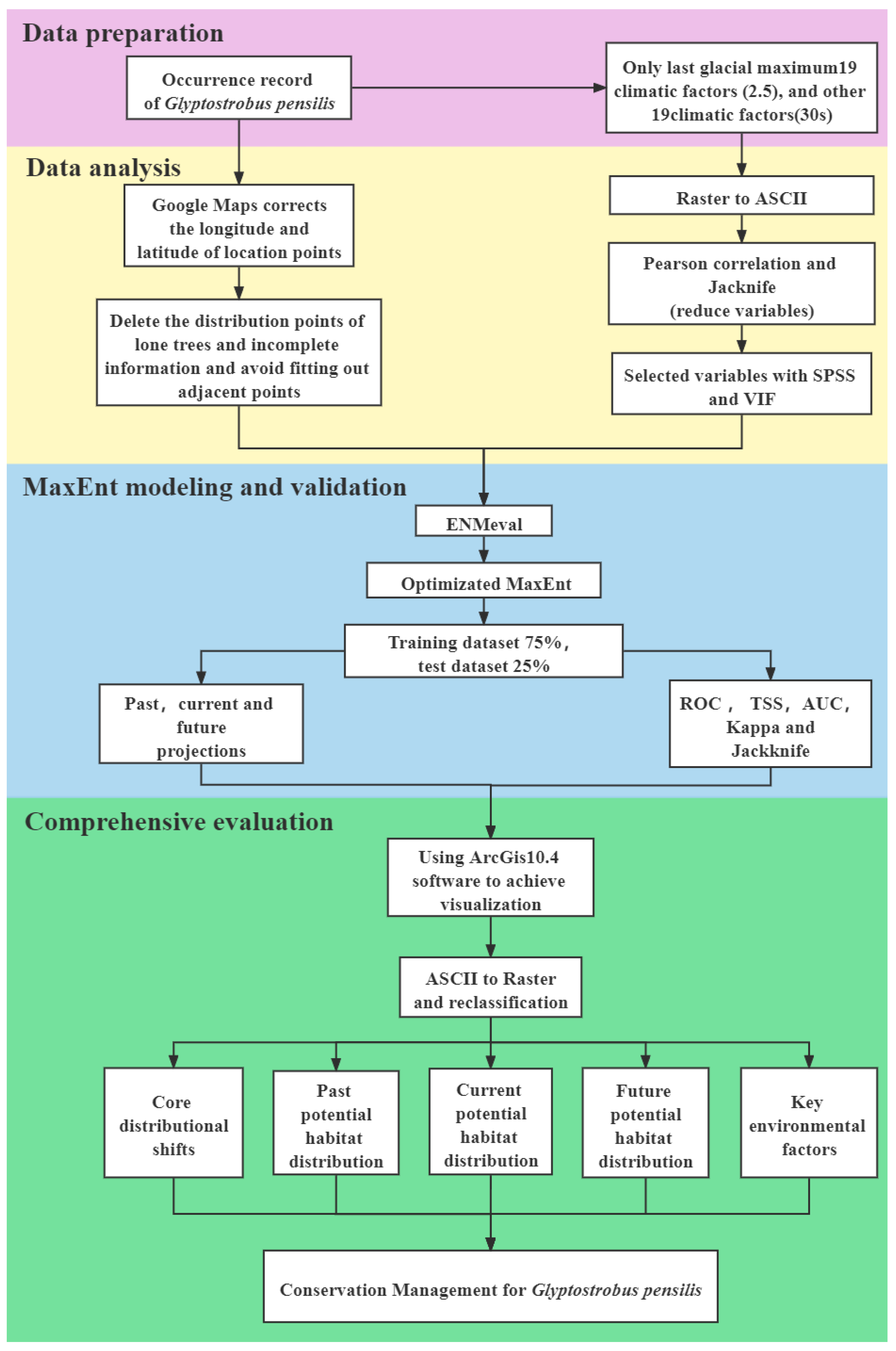
2. Materials and Methods
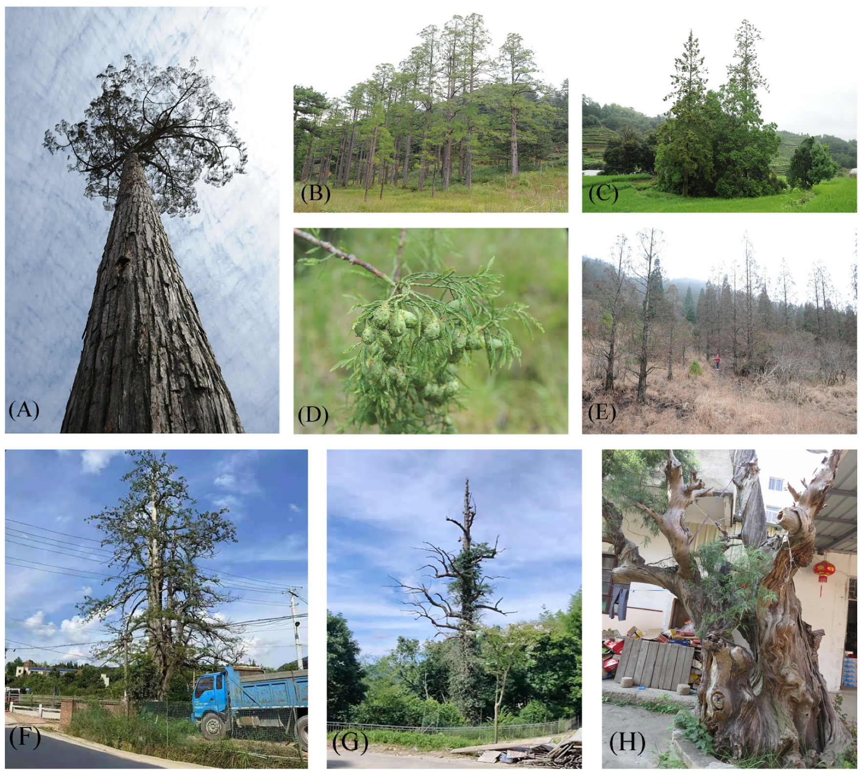
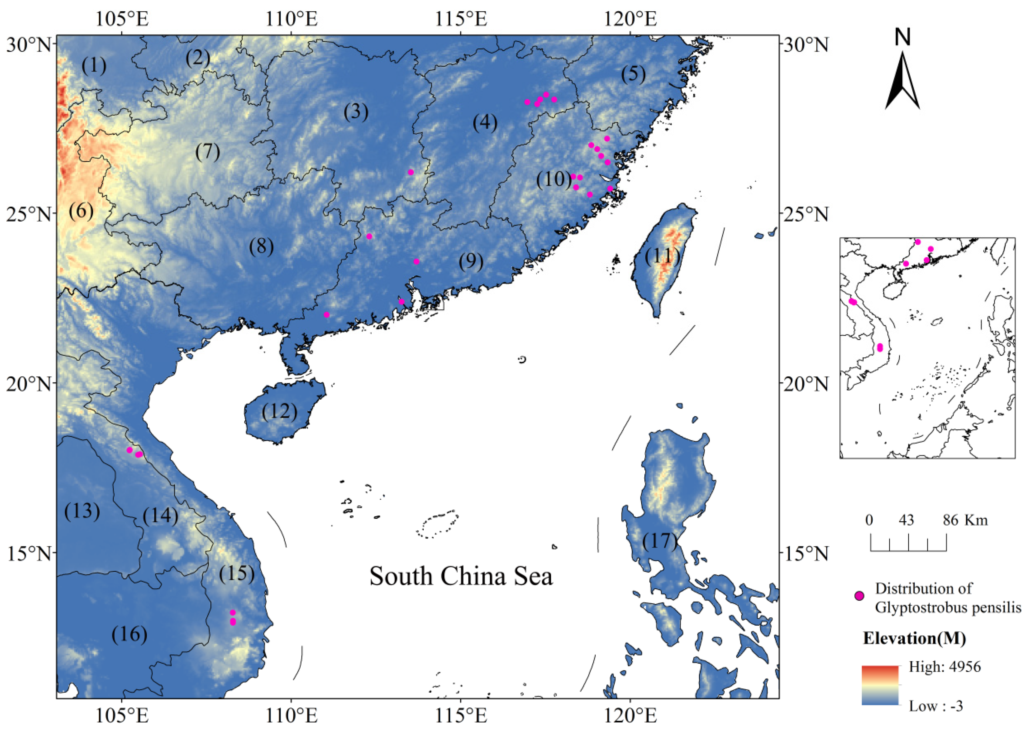
2.1. The Study Area

G. pensilis is an endangered plant under national class I protected plant in China. Its boundaries are the Xinjiang River basin of Jiangxi Province in the North, the South-Central Vietnam in the South, the Jiaoxi River basin of Ningde in Fujian Province in the east and the mountainous area of Southeastern Guizhou and Southeastern Yunnan Province in the west (Figure 2) [27,28,29,30,31,32,33,34,35,36,38,39,40,41,42]. The geographical coordinates of the natural distribution area of G. pensilis are 10°~29° N and 103°~122° E. Because it is necessary to provide reference for artificial introduction and cultivation, 90°–130° E and 0°–35° N were taken as the prediction area. The complete workflow analyzed in this study is summarized in Figure 3.

2.2. Collection and Screening of Sample Data

From 2004 to 2019, Our team (include Bao Liu, Shipin Chen, Shiqun Zheng, Shaoning Ruan, Tianyu Zhang and Xingzhuang Ye) conducted field investigations of the natural population of G. pensilis in Fujian, Jiangxi and Guangdong provinces and collected 24 distribution records [39,40,42]. The published literature was reviewed to collect 9 and 5 records of the population distribution of G. pensilis in Vietnam and Laos, respectively [29,31,34,36,43]. 41 distribution records were collected by consulting the published literature; retrieval of global biodiversity information facility (http://www.gbif.org, last accessed on 8 August 2021) and national specimen information infrastructure (http://www.nsii.org.cn, last accessed on 8 August 2021), yielded 392 and 417 records, respectively, for a total of 863 records. In order to reduce the error, all the above records were screened with reference to the methods of Wu [19] and the distribution points of plantations, incomplete information and isolated trees (no population of G. pensilis was present and trees generally had serious diseases and insect pests or on the verge of death and the representative significance is not strong); in order to reduce the error caused by the clustering effect, only one distribution point is reserved for each grid (10 km × 10 km) and 27 valid samples were finally obtained (Figure 3 and Table S1).

2.3. Environment Variable Filtering and Data Processing

The climate data were downloaded from the WorldClim database (http://worldclim.org, last accessed on 1 July 2021) and selected CCSM4 model climate data of version 1.4 [44]. Except for the last glacial maximum, which has a spatial resolution of 2.5 arc-minute, the other periods have a resolution of 30 arc-second. In order to improve the prediction accuracy, 19 climatic variables from the LIG, Last Maximum Glacial (LGM; about 22 ka), Middle Holocene (MH; about 6000 years ago), current (about 1960~1990), the 2050s (2041~2059) and the 2070s (2061~2079) under representative concentration pathway 2.6 (RCP2.6) and RCP8.5 scenarios were selected [45]. Spearman correlation analysis and the variance inflation factor (VIF) were used to screen out eight climate factors that had a great influence on the distribution of G. pensilis (Table 1).

2.4. Model Building, Optimization and Evaluation

In this study, MaxEnt 3.4.1 (https://biodiversityinformatics.amnh.org/open_source/maxent/, last accessed on 1 July 2021) was used to simulate the potential suitable habitat areas of G. pensilis under the LIG, LGM, MH, current and four scenarios in the future (RCP2.6–2050s RCP2.6–2070s, RCP8.5–2050s and RCP8.5–2070s) [17,46]. In order to make the probability of occurrence close to a normal distribution, 75% of the data were selected for model training, the remaining data were used for model testing and other values were the default values [18,19,20,21]. The EMNeval [41,47] package in R (Cran) version 3.6.1 [48] was used to optimize the MaxEnt model and the regularization multiplier (RM) was set to 0.5–4, with intervals of 0.5 each and a total of 8 regulated frequency multipliers. The MaxEnt model provides five features, which are linear features (L), quadratic features (Q), hinge features (H), product features (P) and threshold features (T). Ten feature combinations (FCs) were adopted: L, QT, H, LQH, LQHP, LQHPT, HPT and QPT. We used ENMeval [41] to test the 80 above-mentioned parameter combinations before finally adopting the minimum information criterion AICc value (delta.AICc) model of the Akaike information criterion, as well as adopting a 10% training omission rate (OR10) and difference between the AUC values (AUCDIFF) to test the fitting degree and complexity of the model. AICc is a standard to measure the accuracy of the model. When the model has the lowest AICc value (delta. AICc = 0), it is called the best model, which can significantly reduce the complexity of the model.
Optimized parameters were used to debug MaxEnt3.4.1 software and then to simulate and predict the suitable habitats of G. pensilis in different periods. The averaged result from 10 replications was taken as the final output. The area under the receiver curve (AUC), Kappa and true skill statistics (TSS) were used to evaluate the accuracy of MaxEnt’s prediction. The AUC value ranged from 0 to 1. The larger the value, the higher the reliability of the distinction between suitable and unsuitable habitats. AUC = 0.5 indicated that the model fails to judge completely, less than 0.8 indicated a low reliability and 0.9~1.0 indicated a high credibility [49]. The evaluation criteria for Kappa value and TSS were excellent, 1.0–0.85; very good, 0.7–0.85; good, 0.55–0.7; fair, 0.4–0.55; fail, <0.4 [50,51,52].
The ASCII format was imported into ArcGis10.4 and converted it into a raster file for visual processing. The author used the reclassify function of ArcGis 10.4 to divide the habitat suitability index (HSI) according to the known distribution pattern of G. pensilis. HIS < 0.2 is a non-suitable habitat, 0.2 ≤ HIS < 0.5 is a generally suitable habitat, 0.5 ≤ HIS < 0.7 is a moderately suitable habitat and HIS ≥ 0.7 is a highly suitable habitat.

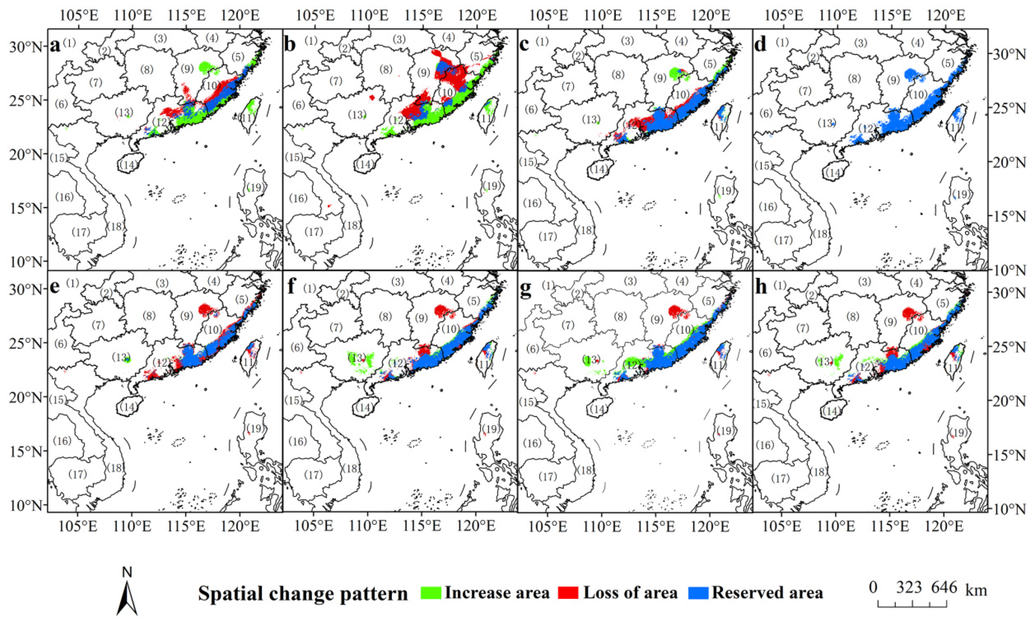
2.5. Analysis of the Spatial Pattern Change and Core Point Migration in the Suitable Habitat Area of Species

We tried five thresholds of 0.5, 0.6, 0.7, 0.75 and 0.8 were tried. It was found that when Q = 0.5 and 0.6, the distribution area was too large; when Q = 0.75 or Q = 0.8, Jiangxi and other large populations become unsuitable areas. When Q = 0.7, although the predicted area is still large, most of G. pensilis populations have been included, which is more reasonable. We considered the value Q ≥ 0.7 as the suitable habitat zone, that is, the suitable includes the generally suitable, the medium suitable and the highly suitable, which is represented by “1”; the logical value Q < 0.7 is regarded as the non-suitable, represented by “0” [21]. We defined four types of changes in the suitable habitats of species: newly increased suitable, lost suitable habitats and reserved suitable and unsuitable. The future area changes were all calculated based on current suitable. The matrix value 0→1 represents the newly increased suitable area, 1→0 represents the lost suitable area, 1→1 represents the reserved suitable area and 0→0 represents the unsuitable area. Finally, the matrix change value was loaded into ArcGis 10.4 to create visualizations of the spatial pattern change of its suitable area. This specific method was obtained from the work of Zhang et al. [53].
Then, the “Zonal Geometry” tool of Arc Gis10.4 was used to calculate the change trend of suitable habitat regions and eight center points of suitable habitat regions—LIG, LGM, MH, Current, RCP2.6-2050s, RCP8.5-2050s, RCP2.6-2070s and RCP8.5-2070s—were compared. After taking the suitable habitat of G. pensilis as a whole and reducing it to a vector particle, the change of centroid position reflected the size and direction of spatial change of suitable habitat. The geosphere package in R Software is used to calculate the core of the habitat migration distance of G. pensilis under 8 climate scenarios [21].

3. Results

3.1. Model Optimization and Accuracy Evaluation

The optimization results show that when FC = LQ and RM = 1, delta.aICC = 0, the model under this parameter is the optimal model (Table S2). Under these parameters, the maximum, minimum and average values of training AUC of 10 repeats were 0.9865, 0.9781 and 0.9815 ± 0.0025, respectively, and the maximum, minimum and average values of test AUC were 0.9985, 0.9581 and 0.9805 ± 0.0112; both kappa and true skill statistics (TSS) are 0.7333, respectively, indicating that the optimized prediction results were high (Table S4, Figures S2–S7).

3.2. Importance of Environment Variables

In terms of the percent contribution, the cumulative proportion of the most important five environmental factors were 95.32%, which was a mean diurnal range (Bio2, 40.59%) and the suitable range was 3.90~10.36 °C. The optimum temperature was −5.65~16.73 °C for the minimum temperature of coldest month (Bio6, 32.86%). The optimal range of annual precipitation (Bio12, 9.24%) was 1175.4~2888.45 mm; the optimal range of the mean temperature of driest quarter (Bio9, 7.79%) was 0.38~25.25 °C; the precipitation of driest month (Bio14, 4.48%) in the most suitable range was 12.22~113.9 mm. The cumulative proportion of the top five factors with permutation importance was as high as 95.57% (Table 1). As it can be seen in Figure S8 that all of the univariate response curves are unimodal, that is, with the increase of the variable, the fitness keeps increasing and when it reaches the maximum value, the fitness keeps decreasing, for example, the value of Bio12 decreased gradually after reaching the peak value at 2035.62.
When only a single variable is used, the variable with the highest regularization training gain is annual precipitation (Bio12); the variable with the highest test gain is annual precipitation (Bio12); the variable with the highest AUC value is Bio12; when using other factors, the variables with the largest decrease in regularization training gain, test gain and AUC value are precipitation of warmest quarter (Bio18); the variable with the largest decrease in AUC value is the minimum temperature of coldest month (Bio6) (Figure S9). In general, the main factors affecting the current geographical distribution of G. pensilis were found to be temperature factors and precipitation factors.

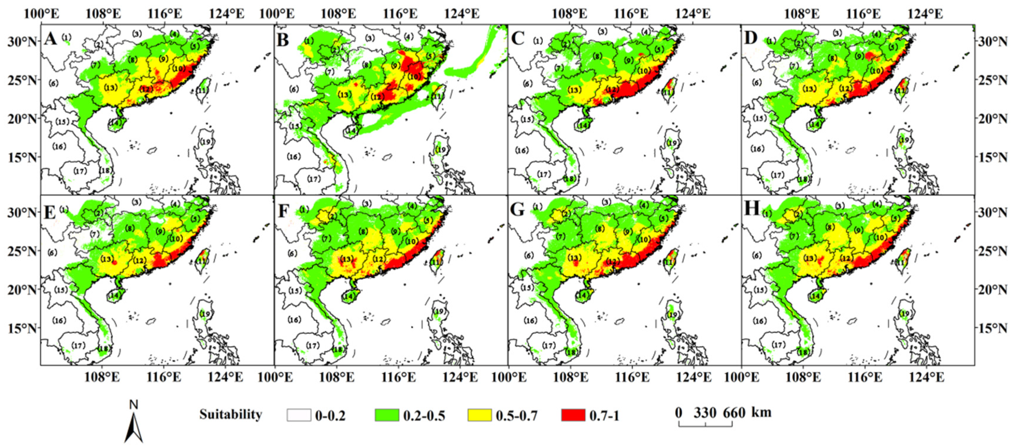
3.3. Current Potential Suitable Habitats

The distribution point ratios of the modern distribution records of G. pensilis belonging to the highly suitable habitats, the moderately suitable habitats and the general suitable habitats are 3.85%, 57.69% and 38.46%, respectively, indicating that the current suitable habitats simulated by MaxEnt can nearly cover the current distribution points. It can be seen from Table 2 that the area of current suitable habitats for G. pensilis was found to be 143.77 × 10⁴ km2, of which the highly suitable habitats was 11.46 × 10⁴ km2. It can be seen from Figure 4d that suitable distribution habitats mainly include Southeast China (mainly includes Fujian, Jiangxi, Zhejiang, Southern Anhui, Chongqing, Hunan, Guangdong, most of Guangxi, Hainan and Taiwan provinces), most of Vietnam and parts of Laos. The highly suitable habitats were found to be located in Eastern Fujian, Northeastern Jiangxi, Eastern Guangdong and the Northern part of Taiwan Provinces. The average suitability of the 27 distribution records was 0.65 and the most suitable place was found to be Fuqing (0.83), Fujian Province and the least suitable place was found to be Dak Lak (0.31), Vietnam.

3.4. Potential Distribution in the Past and Future

During the LIG, the potential suitable habitats were significantly reduced, shrinking by 17.69% compared to the current climate. During this period, Chongqing Municipality and Sichuan Province were unsuitable habitats; the highly suitable habitats, which are mainly distributed in Eastern Fujian Province and Eastern Guangdong Province, shrank by 14.31% compared to the current period, leaving only 9.82 × 10⁴ km2. During the LGM, the potential suitable habitats were significantly increased (43.98% larger than the LIG) and the highly suitable habitats were increased by 18.52% compared to the current period and they were mainly distributed in Fujian Province. The continental shelf of the East China Sea (ECS) and the Taiwan Strait became land during this period and became low suitable habitats for G. pensilis. In the MH, the outline of the potential suitable distribution area of G. pensilis was basically the same as the current one. The highly suitable habitats were mainly located in the Eastern coastland of Fujian Province and the Northeastern part of Guangdong Province. The highly suitable area was increased by 11.08% compared to the current period (Figure 4, Figure 5 and Table 2).
In the next four periods, the range of highly suitable habitats will be relatively stable, mainly including Eastern Fujian province and Eastern Guangdong province. Unfortunately, northeastern Jiangxi province is no longer a highly suitable habitats (Figure 4 and Figure 5). For the RCP2.6-2050s scenario, the area of the highly suitable habitats has sharply shrunk, leaving only 8.86 × 10⁴ km2, a reduction of 22.69% compared to the current (Table 2). For the RCP8.5-2050s scenario, the high and moderately suitable habitats are most fragmented, the suitable habitats are 16.80% larger than the current, but the highly suitable habitats decreased by 4.28% compared with the current. For the RCP2.6-2070s scenario, the highly suitable habitat expanded instead, with an area of 12.99 × 10⁴ km2, 13.35% larger than that in current. For the RCP8.5-2070s scenario, the moderately suitable habitats are 60.56% larger than the current period and the highly suitable habitats are 9.95% smaller than the current period (Table S4).

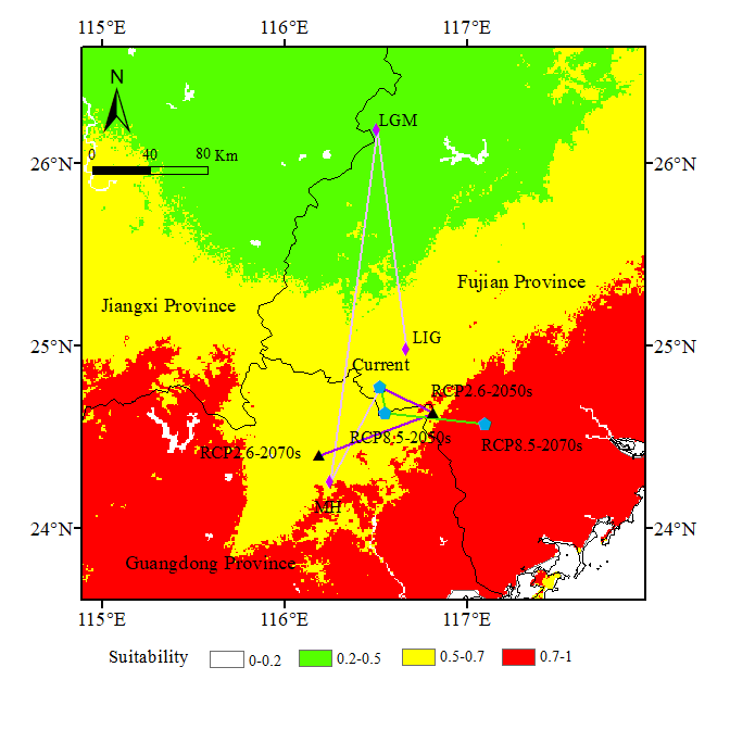
3.5. Shifts of the Core Suitable Habitat Distributions under Climate Change Scenarios

During the three paleoclimate periods, the core of the LIG suitable habitat was located in Taiba Town, Shanghang County, Fujian Province, and then the centroid of the LGM moved northwest to Huaitu Town, Ninghua County, Fujian Province, with a distance of 134.87 km from LIG (Figure 6). During the MH, the core of the habitat migrated southwest to Xiyang Town, Meijiang District, Meizhou City, Guangdong Province, with a distance of 215.74 km from the LGM. The current habitat centroid position of G. pensilis was estimated to be in Hongshan Township, Yongding District, Longyan City, Fujian Province, which shifted northeast to 63.62 km relative to the MH. Under RCP2.6-2050s, the core of the habitat was in Xiayang Town, Yongding District, Longyan City, Fujian Province. Compared with the current period, it migrated 33.57 km to the southeast. Under RCP2.6-2070s, the core of the habitat further migrated 183.14 km to the southwest, it located in Shuyang Town, Nanjing County, Fujian Province. Under RCP8.5-2050s, the core of the habitat was in Fengshi Town, Yongding District, Longyan City, Fujian Province. Compared with the current period, it shifted 16.30 km south. Under RCP8.5-2070s, its habitat centroid further migrated 55.98 km to the southeast and the core of the habitat was located in Shuyang Town, Nanjing County, Zhangzhou City, Fujian Province. In the future, the total suitable areas of G. pensilis will migrate to lower latitudes and the migration position will further expand southward.

4. Discussion

4.1. The Change Pattern of Potential Distribution Area

This study predicts that the Fujian and Guangdong provinces contains the highly suitable habitats for the LIG and the LGM. The highly suitable habitats for the LGM of G. pensilis expanded to the continental shelf of the ECS and the South China Sea (SCS). There is a large number of relict plants such as Ginkgo Biloba, Taxus wallichiana var. mairei, Tsuga chinensis, Tsoongiodendron odorum, Cycas taiwaniana, Cycas fairylakea, Sphaeropteris lepifera and G. pensilis in Fujian and Guangdong provinces, and no cold fauna fossils have been found [54,55]. In addition, due to the low latitude and low mountains in Fujian and Guangdong, the temperature and altitude conditions for glacier formation could not be reached during the glacial period, and no glacier relics have been found in these two areas [54,55,56,57]. Since the Pleistocene, the warm and humid climate and diverse mountain conditions in Fujian and Guangdong provinces have become the climate refugium sanctuary of many endangered plants [55,56,57,58,59]. The vegetation of the LGM in Fujian comprises subtropical evergreen broad-leaved forests and warm temperate deciduous forests in Fujian and Guangdong provinces [55,56,60,61]. After the Younger Dryas (about 12.5–11.5 kaBP) event, a large number of marshlands appeared in Fujian, which was particularly suitable for the habitat requirements of G. pensilis [58,62]. Rare populations of G. pensilis were found in Youxi County, Pingnan County and Zhouning County of Fujian Province and it was scattered in more than 30 counties of Fujian and Guangdong provinces (Figure S10) [30,32,34,39,42]. Therefore, it was reasonable and credible for MaxEnt to predict that the highly suitable habitats of G. pensilis during the LIG and the LGM is mainly located in Fujian and Guangdong. During the LGM, the sea level of the ECS and SCS dropped by about 120~130 m, so most of the continental shelves were exposed to the sea [63]. Moreover, the winter temperature in the coastland of South China was 11~15 °C lower than that of the current and the role of winter wind was strong [64]. During the Quaternary glacial period, the vegetation of sparse forest and grass, dominated by Cyperaceae and Artemisia, developed on the continental shelf of the ECS and there may have been Gymnospermous plants including the Taxodiaceae in the surrounding regions [65,66]. In Qianhu Bay of Zhangpu County, Fujian Province, ancient trees such as G. pensilis were excavated before 42 ka BP [67]. The fossil species of Glyptostrobus was widespread throughout Eurasia and North America during the Tertiary period [28,35]. In the late Tertiary, especially after the Quaternary glaciation, the temperature decreased, the species’ distribution region strongly shrank and moved southward and it became extinct in North America and Europe but was preserved in some regions south of the Yangtze River Basin (China), Laos and Vietnam that were less affected by the glaciation [68,69,70,71,72]. Zheng et al. [73] also showed that the trees of G. pensilis were widely distributed in the exposed continental shelf of the ECS and the northern continental shelf of the SCS during the LGM. Therefore, during the LGM, the ECS shelf and the northern continental shelf of the SCS were likely to have been suitable habitats for G. pensilis and the highly suitable habitats for G. pensilis was mainly located in Fujian and Guangdong provinces. During the period of MH, the climate tended to be warm and humid and the vegetation and climate conditions in Southern China may have been close to the current. The evergreen broad-leaved forest was the main vegetation type in this period [74]. Sedimentary profile analysis showed strong summer monsoon, abundant precipitation and humid climate conditions during 10~3.3 cal kaBP in the Tianhushan region, Fujian Province, China [75]. The Zhaoqing district has experienced five stages of evergreen broad-leaved forest—G. pensilis forest swamp, evergreen broad-leaved forest, grassland swamp, secondary forest and grassland farmland, in turn—since the MH [76]. Fossil and sporopollen records show that G. pensilis was widely distributed in South China in the middle and late Holocene [77]. Thus, G. pensilis may have recovered growth in this period and the potential suitable habitats of medium and high height may have been slightly larger than those of current.
The continental shelf of the ECS during the LGM was a suitable area for G. pensilis, which indicates that it may have retreated from Japan to the south via the ECS continental shelf to take refuge in Jiangxi, Fujian and Guangdong Province. Previous studies have shown that the genetic diversity level of G. pensilis in Fujian is relatively high [29,42], as well as that Fujian Province has always been a highly suitable area during the LIG, LGM and MH. Thus, it was speculated that the Fujian District was likely to have been the climate refugium of. G. pensilis.
Cao et al. [78] analyzed the current and future suitability zones of six endangered wetland species in China, including G. pensilis and revealed that the highly suitable zones of G. pensilis are southeastern China (about Fujian, Guangdong, most of Hainan, Northeast Jiangxi and most of Taiwan), which is consistent with the conclusion of the present study. In addition, the potential reserved suitable habitat area obtained in this study can lay a theoretical foundation for the construction of G. pensilis plantation. When the future greenhouse gas emission scenarios were RCP8.5-2050s, RCP2.6-2070s and RCP8.5-2070s, MaxEnt predicted that the potential distribution area of G. pensilis will move southward as a whole. This is because the future increase in temperature and precipitation in the lower latitudes of the southeast coast with climate warming may provide a more suitable growth environment for G. pensilis. This may also be related to the excessive Percent Contribution (PC) of bio6 (PC is 32.86%, ranking second), because the main role of this factor may be to limit the northward migration of species. The suitable areas of many endangered plants such as Thuja sutchuenensis [79] and Larix kaempferi [80] all showed significant shrinkage in the future, which was consistent with the conclusion of this study.

4.2. Constraints of Climatic Factors on Geographical Distribution

This study shows that temperature is more important than precipitation in controlling the distribution pattern of G. pensilis and Wu [42] also draws the same conclusion. The percent contribution of the temperature factor was found to be as high as 81.91%, so the influence of the temperature factor is relatively greater than that of the precipitation factor. Studies have shown that G. pensilis has very strict habitat requirements and poor resistance to extreme climate. The seedlings cannot withstand low temperature and the plant will wither and die in a lasting 0 °C environment. Additionally, extreme low temperatures (below −5.3 °C) lead to frost damage for G. pensilis. It is suitable to grow in an environment with an annual average temperature of 15–22 °C [40] and abundant precipitation. The optimal annual rainfall is 1199.6–2231 mm [55], which is close to the threshold value given by the results of this study. This is inconsistent with the conclusion of this study. The MaxEnt analysis results showed that the replacement importance value of the minimum temperature of coldest month (Bio6) and mean temperature of driest quarter (Bio9) were the highest regularization training gains using this factor alone. Previous studies have shown that the temperature factor has an irreplaceably restrictive effect on the distribution pattern of plants and, in many cases, the temperature factor is still the primary restrictive factor, especially for southern plants [42,60,78,81,82,83,84]. Li et al. [30] found that although G. pensilis can withstand low temperatures, it is susceptible to freezing damage if low temperatures last for a long time, which seriously inhibits its growth. In conclusion, low temperatures in winter may be the key factor restricting the northward seed dispersal of G. pensilis. The cold environment causes G. pensilis to fail to bear fruit, which makes it unable to complete its life cycle in the north [30,42]. This further indicates that the temperature factor is the leading factor restricting the distribution of G. pensilis. Metasequoia glyptostroboides, a sibling species of G. pensilis, is mainly restricted by the precipitation of driest month (Bio14), the precipitation of wettest quarter (Bio16), the precipitation of wettest month (Bio13) and the mean temperature of wettest quarter (Bio8), though this leads to conclusions inconsistent with this study [83], because M. glyptostroboides is only distributed at the junction of Hunan, Hubei and Chongqing Provinces, with small longitude, latitude and temperature differences. This tree species grows in wet habitats, but seed germination and seedling survival are low when seeds fall into swamps, so that seedlings are only established during periods of low water [39,61,86,87]. Several studies have shown that G. pensilis cannot survive in water-deficient habitats [40,42,87]. According to the conclusion of this study, the authors also boldly speculate that the winter precipitation has been limiting G. pensilis from crossing the Wushan-Wuling-Ailao Mountain to Yunnan, Guizhou and Sichuan Provinces.

4.3. Conservation Management

The genetic diversity level of G. pensilis is extremely low and its genetics are highly differentiated; most G. pensilis plants grow separately and discontinuously [29,42,88,89,90,91,92]. The level of genetic diversity is proportional to the adaptability of species. Some experts believe that if no effective protection measures are taken, G. pensilis will be extinct within 100 years and face the plight of “nowhere to go” [77,91]. Therefore, based on the conclusion of this study, the following protective measures are formulated:
The delayed response of gymnosperms to climate change may lead to distribution shrinkage or even extinction [91,92]. For example, Wu’s study showed that about 41% of 109 gymnosperms will be at risk of extinction due to climate change [88]. Due to gymnosperms low migration rate, serious fragmentation of suitable habitats and frequent human activities, it may not be able to quickly adapt to suitable range changes. Therefore, G. pensilis within and outside nature reserves must be managed through in situ and ex situ conservation, habitat wetland conservation, assisted migration and sapling conservation to avoid extinction [29,42,49,77,93].
For the newly increased suitable habitats, rational and sustainable land use planning should be conducted while considering that G. pensilis is mostly distributed along marshes and rivers and so planners should reserve enough space for G. pensilis’s migration. The new suitable habitats are scattered in the marginal areas of the suitable habitats and it is necessary to reduce human disturbance activities in these areas and increase the possibility of G. pensilis migration. In addition, its seeds are large and heavy, requiring artificially assisted migration to facilitate their dispersal and colonization.
For the lost suitable habitats, ex situ protection measures should be actively taken, botanical gardens should be established and G. pensilis should be transplanted into artificial environments for cultivation, conservation and preservation. Because it is suitable for cultivation in the middle and lower reaches of warm and humid rivers. For example, the construction of G. pensilis plantations in Jiangmen Nature Reserve is better [56] and the relocation protection mainly cultivates seedlings by transplanting large seedlings, seeds and asexual reproduction. It is necessary to establish the population number that can maintain its genetic diversity at the protection point [94]. However, the results of this study show that under the future four climate scenarios (Figure 4e–h), the climatic conditions in Laos, Vietnam and northeast Jiangxi are not suitable for the growth and development of G. pensilis. It is suggested to increase investment in special funds and actively carry out studies on reproductive biology, molecular mechanisms of stress resistance (e.g., drought stress), population ecology and artificial domestication of G. pensilis, so as to promote the natural regeneration of the above natural populations and avoid the risks of genetic adaptability variation, mutation accumulation and loss of genetic resources.
Under future climate change conditions, the reserved suitable habitats can be used as the safety and climate refugia of G. pensilis to cope with climate change, which is of great importance. Therefore, more attention should be paid to the protection and management of reserved area. Studies have shown that the exotic plant invasion of existing G. pensilis species is relatively serious [34,42,93]. The minimization of human harmful interference factors and the threat of alien plant invasion against G. pensilis communities can improve the health levels of the species and individuals [77,93]. Thus, the stability of resistance and resilience of G. pensilis populations can be improved, to protect it, first of all, it is necessary to protect the surrounding habitat of the existing community, as well as to restore and expand the wetland areas around the communities. In addition, the establishment of nature reserves is the most effective method for the in situ protection of rare and endangered wildlife resources [29,42,90]. The current distribution of G. pensilis is concentrated in Vietnam, Laos and Southeast China (mainly includes Jiangxi, Guangdong and Fujian), so these places may be suitable habitats for the plant and should be the focus of future conservation efforts.

5. Conclusions

The suitable habitats of G. pensilis include Vietnam, Laos and South China. Historically, this species experienced significant range expansion during LIG and LGM, but the range contracted slightly during MH, which was similar to the current suitable area. Under various future climate scenarios, there will be potential for different levels of contraction and highly suitable districts will trend towards lower latitudes. Wetlands, an important habitat that is suitable for the distribution of G. pensilis, is shrinking each year. As a result, the species are likely to face the plight of “nowhere to go”. Our study provides an important reference for the conservation of G. pensilis and other endangered wetland species under climate change.

Supplementary Materials

The following supporting information can be downloaded at: https://www.mdpi.com/article/10.3390/f13020257/s1, Figure S1: avg.diff.AUC; Figure S2: avg.test.AUC; Figure S3: avg.test.or10pct; Figure S4: avg.test.orMTP; Figure S5: delta.AICc; Figure S6: Analysis of omission commission; Figure S7: the receiver operating characteristic (ROC) curve; Figure S8: Average response curves of eight predictor variables of the modeled distribution of G. pensilis based on the MaxEnt model. (A) Bio1; (B) Bio2; (C) Bio6; (D) Bio9; (E) Bio12; (F) Bio14; (G) Bio15; (H) Bio18. The variable codes are the same as those in Table 1; Figure S9: Jackknife test for the importance of environmental variables.(A) Reguarized training gain; (B) Test gain; (C) AUC; The variable codes are the same as those in Table 1; Figure S10: Photos of G. pensilis in different areas of Fujian Province; Table S1: 27 species presence data for MaxEnt modeling; Table S2: Evaluation metrics of Maxent model generated by ENMeval; Table S3: The mean area under the curve (AUC) from 10 replicate models of Glyptostrobus pensilis under three past, present and eight future climate scenarios; Table S4: Change rate of suitable habitats areas of G. pensilis under different climate change.

Author Contributions

Conceptualization, X.Y.; methodology, X.Y.; software, X.Y., W.L., M.Z., G.W., Q.Y. and Y.L.; validation, X.Y., M.Z., Q.Y. and L.Y.; formal analysis, X.Y., Q.Y. and M.Z.; investigation, B.L., S.C., G.Z., S.Z., X.Y., W.L., M.Z., Y.L., Y.L., S.R. and T.Z.; resources, X.Y., G.Z., S.C. and B.L.; data curation, X.Y. and B.L.; writing—original draft preparation, X.Y.; W.L., M.Z., Q.Y. and L.Y. writing—review and editing, X.Y.; visualization, X.Y. and M.Z.; supervision, X.Y., W.L. and B.L.; project administration, B.L.; funding acquisition, B.L. All authors have read and agreed to the published version of the manuscript.

Funding

The second national key protected wild plant resources survey and research (China, KH140126A); National Forestry; Grassland Administration Science and Technology Program (China, KJZXSA2018008); Fuzhou-Dingxi East-West Poverty Alleviation Collaborative Soil Erosion Comprehensive Control Project (KH180062A) and Key research and development project of Ningxia Hui Autonomous Region, China (2019BBF02025).

Institutional Review Board Statement

Not applicable.

Informed Consent Statement

Not applicable.

Data Availability Statement

Not applicable.

Acknowledgments

We thank the contributors to the databases used in this study. We also appreciate the help from Huai-qing Huang in the field investigation at Youxi Jiufushan Nature Reserve; Ze-yan Wu and Ji-ce Lu in the field investigation at Pingnan County, Fujian Province; and Si-zhong Luo in the field investigation at Yiyang County, Jiangxi Province. We are thankful to three anonymous Reviewer for valuable and helpful comments which greatly improved the manuscript.

Conflicts of Interest

The authors declare no conflict of interest.

References

  1. Armenise, L.; Simeone, M.C.; Piredda, R.; Schirone, B. Validation of DNA barcoding as an efficient tool for taxon identification and detection of species diversity in Italian conifers. Eur. J. For. Res. 2012, 131, 1337–1353. [Google Scholar] [CrossRef]
  2. Crisp, M.D.; Cook, L.G. Cenozoic extinctions account for the low diversity of extant gymnosperms compared with angiosperms. New Phytol. 2011, 192, 997–1009. [Google Scholar] [CrossRef]
  3. Wu, F.; Dai, S.J.; Vlasak, J.; Spirin, V.; Dai, Y.C. Phylogeny and global diversity of Porodaedalea, a genus of gymnosperm pathogens in the Hymenochaetales. Mycologia 2019, 111, 40–53. [Google Scholar] [CrossRef] [PubMed]
  4. Yang, Y.; Liu, B.; Dennis, M.N. Red list assessment and conservation status of gymnosperms from China. Biodivers. Sci. 2017, 25, 758–764. [Google Scholar] [CrossRef] [Green Version]
  5. Paik, I.S.; Lee, Y.I.; Kim, H.J.; Huh, M. Time, space and structure on the korea cretaceous dinosaur coast: Cretaceous stratigraphy, geochronology, and paleoenvironments. Ichnos 2012, 19, 6–16. [Google Scholar] [CrossRef]
  6. Mantzouka, D.; Sakala, J.; Kvacek, Z.; Koskeridou, E.; Ioakim, C. Two fossil conifer species from the neogene of alonissos island (iliodroma, greece). Geodiversitas 2019, 41, 125–142. [Google Scholar] [CrossRef] [Green Version]
  7. Keller, G.; Mateo, P.; Monkenbusch, J.; Thibault, N.; Punekar, J.; Spangenberg, J.E.; Abramovich, S.; Ashckenazi-Polivoda, S.; Schoene, B.; Eddy, M.P.; et al. Mercury linked to deccan traps volcanism, climate change and the end-cretaceous mass extinction. Glob. Planet. Chang. 2020, 194, 17. [Google Scholar] [CrossRef]
  8. Eiserhardt, W.L.; Borchsenius, F.; Sandel, B.; Kissling, W.D.; Svenning, J.C. Late cenozoic climate and the phylogenetic structure of regional conifer floras world-wide. Glob. Ecol. Biogeogr. 2015, 24, 1136–1148. [Google Scholar] [CrossRef]
  9. Zheng, Y.; Liu, J.; Feng, X.Y.; Gong, X. The distribution, diversity, and conservation status of cycas in China. Ecol. Evol. 2017, 7, 3212–3224. [Google Scholar] [CrossRef]
  10. McCallum, M.L. Turtle biodiversity losses suggest coming sixth mass extinction. Biodivers. Conserv. 2021, 30, 1257–1275. [Google Scholar] [CrossRef]
  11. Elewa, A.M.T.; Abdelhady, A.A. Past, present, and future mass extinctions. J. Afr. Earth Sci. 2020, 162, 103678. [Google Scholar] [CrossRef]
  12. Barnosky, A.D.; Matzke, N.; Tomiya, S.; Wogan, G.O.U.; Swartz, B.; Quental, T.B.; Marshall, C.; McGuire, J.L.; Lindsey, E.L.; Maguire, K.C.; et al. Has the earth’s sixth mass extinction already arrived? Nature 2011, 471, 51–57. [Google Scholar] [CrossRef]
  13. Cursach, J.; Moragues, E.; Rita, J. The key role of accompanying species in the response of the critically endangered Naufraga balearica (Apiaceae) to climatic factors. Plant Ecol. 2018, 219, 561–576. [Google Scholar] [CrossRef]
  14. Qiu, C.J.; Shen, Z.H.; Peng, P.H.; Mao, L.F.; Zhang, X.S. How does contemporary climate versus climate change velocity affect endemic plant species richness in China? Chin. Sci. Bull. 2014, 59, 4660–4667. [Google Scholar] [CrossRef]
  15. Yang, Z.B.; Bai, Y.; Alatalo, J.M.; Huang, Z.D.; Yang, F.; Pu, X.Y.; Wang, R.B.; Yang, W.; Guo, X.Y. Spatio-temporal variation in potential habitats for rare and endangered plants and habitat conservation based on the maximum entropy model. Sci. Total Environ. 2021, 784, 13. [Google Scholar] [CrossRef]
  16. Phillips, S.J.; Dudik, M. Modeling of species distributions with maxent: New extensions and a comprehensive evaluation. Ecography 2008, 31, 161–175. [Google Scholar] [CrossRef]
  17. Merow, C.; Smith, M.J.; Silander, J.A. A practical guide to maxent for modeling species’ distributions: What it does, and why inputs and settings matter. Ecography 2013, 36, 1058–1069. [Google Scholar] [CrossRef]
  18. Garza, G.; Rivera, A.; Barrera, C.S.V.; Martinez-Avalos, J.G.; Dale, J.; Arroyo, T.P.F. Potential Effects of Climate Change on the Geographic Distribution of the Endangered Plant Species Manihot walkerae. Forests 2020, 11, 689. [Google Scholar] [CrossRef]
  19. Wu, Y.M.; Shen, X.L.; Tong, L.; Lei, F.W.; Mu, X.Y.; Zhang, Z.X. Impact of past and future climate change on the potential distribution of an endangered montane shrub Lonicera oblata and its conservation implications. Forests 2021, 12, 125. [Google Scholar] [CrossRef]
  20. Su, H.Y.; Bista, M.; Li, M.S. Mapping habitat suitability for Asiatic black bear and red panda in Makalu Barun National Park of Nepal from Maxent and GARP models. Sci. Rep. 2021, 11, 14135. [Google Scholar] [CrossRef]
  21. Ye, X.Z.; Zhao, G.H.; Zhang, M.Z.; Cui, X.Y.; Fan, H.H.; Liu, B. Distribution pattern of endangered plant Semiliquidambar cathayensis (Hamamelidaceae) in response to climate change after the last interglacial period. Forests 2020, 11, 125. [Google Scholar] [CrossRef]
  22. Mai, J.F.; Xian, Y.Y.; Liu, G.L. Predicting potential rainfall-triggered landslides sites in Guangdong Province (China) using MaxEnt model under climate changes scenarios. J. Geo-Inf. Sci. 2021, 23, 2042–2054. [Google Scholar] [CrossRef]
  23. Pandit, K.; Smith, J.; Quesada, T.; Villari, C.; Johnson, D.J. Association of Recent Incidence of Foliar Disease in Pine Species in the Southeastern United States with Tree and Climate Variables. Forests 2020, 11, 1155. [Google Scholar] [CrossRef]
  24. Ning, H.; Tang, M.; Chen, H. Impact of climate change on potential distribution of chinese white pine beetle dendroctonus armandi in China. Forests 2021, 12, 14. [Google Scholar] [CrossRef]
  25. Yang, X.H.; Jin, X.B.; Zhou, Y.K. Wildfire Risk Assessment and Zoning by Integrating Maxent and GIS in Hunan Province, China. Forests 2021, 12, 1299. [Google Scholar] [CrossRef]
  26. De Sousa, V.A.; Reeves, P.A.; Reilley, A.; de Aguiar, A.V.; Stefenon, V.M.; Richards, C.M. Genetic diversity and biogeographic determinants of population structure in Araucaria angustifolia (bert.) o. Ktze. Conserv. Genet. 2020, 21, 217–229. [Google Scholar] [CrossRef] [Green Version]
  27. Yan, Y.D.; Li, X.Y.; Worth, J.R.P.; Lin, X.Y.; Ruhsam, M.; Chen, L.; Wu, X.T.; Wang, M.Q.; Thomas, P.I.; Wen, Y.F. Development of chloroplast microsatellite markers for Glyptostrobus pensilis (cupressaceae). Appl. Plant Sci. 2019, 7, 6. [Google Scholar] [CrossRef] [Green Version]
  28. Richards, K.; Mudie, P.; Rochon, A.; Athersuch, J.; Bolikhovskaya, N.; Hoogendoorn, R.; Verlinden, V. Late pleistocene to holocene evolution of the Emba Delta, Kazakhstan, and coastline of the north-eastern Caspian Sea: Sediment, ostracods, pollen and dinoflagellate cyst records. Palaeogeogr. Palaeocl. 2017, 468, 427–452. [Google Scholar] [CrossRef]
  29. Wu, X.; Ruhsam, M.; Wen, Y.; Thomas, P.; Worth, J.R.P.; Lin, X.; Wang, M.; Li, X.; Chen, L.; Lamxay, V.; et al. The last primary forests of the tertiary relict Glyptostrobus pensilis contain the highest genetic diversity. Forestry 2020, 93, 359–375. [Google Scholar] [CrossRef]
  30. Li, F.G.; Xia, N.H. The geographical distribution and cause of threat to Glyptostrobus pensilis (Taxodiaceae). J. Trop. Subtrop. Bot. 2004, 12, 13–20. [Google Scholar] [CrossRef]
  31. Averyanov, L.V.; Phan, K.L.; Nguyen, T.H.; Nguyen, S.K.; Nguyen, T.V.; Pham, T.D. Preliminary observation of native Glyptostrobus pensilis (Taxodiaceae) stands in Vietnam. Taiwania 2009, 54, 191–212. [Google Scholar] [CrossRef]
  32. Lepage, B.A. The taxonomy and biogeographic history of Glyptostrobus Endlicher (Cupressaceae). Bull. Peabody Mus. Nat. Hist. 2007, 48, 359–426. [Google Scholar] [CrossRef]
  33. Chen, Y.Q.; Wang, R.J.; Zhu, S.S.; Jiang, A.L.; Zhou, L.X. Population status and conservation strategy of the rare and endangered plant Glyptostrobus pensilis in Guangzhou. Trop. Geogr. 2016, 36, 944–951. [Google Scholar] [CrossRef]
  34. Tang, C.Q.; Yang, Y.C.; Momohara, A.; Wang, H.C.; Luu, H.T.; Li, S.F.; Song, K.; Qian, S.H.; LePage, B.; Dong, Y.F.; et al. Forest characteristics and population structure of Glyptostrobus pensilis, a globally endangered relict species of southeastern China. Plant Divers. 2019, 41, 237–249. [Google Scholar] [CrossRef]
  35. Ma, S.Y. Study on Protection and Breeding of Germplasm Resources and Application in Plant Landscaping of the Glyptostrobus pensilis; Zhejiang University: Hangzhou, China, 2020; pp. 1–43. [Google Scholar]
  36. Zhang, Y.M.; Yin, R.T.; Jia, R.R.; Yang, E.H.; Xu, H.M.; Tan, N.H. A new abietane diterpene from Glyptostrobus pensilis. Fitoterapia 2010, 81, 1202–1204. [Google Scholar] [CrossRef]
  37. Mao, D.H.; Wang, Z.M.; Wu, J.G.; Wu, B.F.; Zeng, Y.; Song, K.S.; Yi, K.P.; Luo, L. China’s wetlands loss to urban expansion. Land Degrad. Dev. 2018, 29, 2644–2657. [Google Scholar] [CrossRef]
  38. Dorken, V.M.; Rudall, P.J. Understanding the cone scale in Cupressaceae: Insights from seed-cone teratology in Glyptostrobus pensilis. Peer J. 2018, 6, e4948. [Google Scholar] [CrossRef] [PubMed]
  39. Zheng, S.Q.; Liu, J.F.; Wu, Z.Y.; Fu, D.L.; He, Z.S.; Dai, L.C.; Lu, J.C. The interspecific competition of main population in Glyptostrobus pensilis natural forest in Pingnan County. J. Fujian Coll. For. 2008, 28, 216–219. [Google Scholar] [CrossRef]
  40. Zheng, S.Q.; Wu, Z.Y.; Liu, J.F.; Hong, W.; He, Z.S.; Xu, D.W. The endangering causes and protection strategies for Glyptostrobus pensilis, an endemic relict plant in China. Subtrop. Agric. Res. 2011, 7, 217–220. [Google Scholar] [CrossRef]
  41. Muscarella, R.; Galante, P.J.; Soley-Guardia, M.; Boria, R.A.; Kass, J.M.; Uriarte, M.; Anderson, R.P. Enmeval: An r package for conducting spatially independent evaluations and estimating optimal model complexity for maxent ecological niche models. Methods Eco. Evol. 2014, 5, 1198–1205. [Google Scholar] [CrossRef]
  42. Wu, Z.Y. Study on Conservation Biology and Restoration Technique of the Relict Plant Glyptostrobus pensilis; Fujian Agriculture and Forestry University: Fuzhou, China, 2011; pp. 25–39. [Google Scholar]
  43. Loc, P.K.; The, P.V.; Long, P.K.; Regalado, J.; Averyanov, L.V.; Maslin, B. Native conifers of Vietnam—A review. Pak. J. Bot. 2017, 49, 2037–2068. [Google Scholar]
  44. Gent, P.R.; Danabasoglu, G.; Donner, L.J.; Holland, M.M.; Hunke, E.C.; Jayne, S.R.; Lawrence, D.M.; Neale, R.B.; Rasch, P.J.; Vertenstein, M.; et al. The community climate system model version 4. J. Clim. 2011, 24, 4973–4991. [Google Scholar] [CrossRef]
  45. Wang, Y.Y.; Chao, B.X.; Dong, P.; Zhang, D.A.; Yu, W.W.; Hu, W.J.; Ma, Z.Y.; Chen, G.C.; Liu, Z.H.; Chen, B. Simulating spatial change of mangrove habitat under the impact of coastal land use: Coupling maxent and dyna-clue models. Sci. Total Environ. 2021, 788, 147914. [Google Scholar] [CrossRef] [PubMed]
  46. Hijmans, R.J.; Cameron, S.E.; Parra, J.L.; Jones, P.G.; Jarvis, A. Very high resolution interpolated climate surfaces for global land areas. Int. J. Clim. 2005, 25, 1965–1978. [Google Scholar] [CrossRef]
  47. Shi, X.D.; Yin, Q.; Sang, Z.Y.; Zhu, Z.L.; Jia, Z.K.; Ma, L.Y. Prediction of potentially suitable areas for the introduction of Magnolia wufengensis under climate change. Ecol. Indic. 2021, 127, 14. [Google Scholar] [CrossRef]
  48. R Development Core Team. 2019. Available online: https://Cran.R-Project.Org/Manuals.Html (accessed on 5 January 2021).
  49. Yang, L.; Li, H.E.; Li, Q.; Guo, Q.Q.; Li, J.R. Genetic diversity analysis and potential distribution prediction of Sophora moorcroftiana endemic to Qinghai–Tibet Plateau, China. Forests 2021, 12, 1106. [Google Scholar] [CrossRef]
  50. Allouche, O.; Tsoar, A.; Kadmon, R. Assessing the accuracy of species distribution models: Prevalence, kappa and the true skill statistic (TSS). J. Appl. Ecol. 2006, 43, 1223–1232. [Google Scholar] [CrossRef]
  51. Roberts, D.R.; Bahn, V.; Ciuti, S.; Boyce, M.S.; Elith, J.; Guillera-Arroita, G.; Hauenstein, S.; Lahoz-Monfort, J.J.; Schroder, B.; Thuiller, W.; et al. Cross-validation strategies for data with temporal, spatial, hierarchical, or phylogenetic structure. Ecography 2017, 40, 913–929. [Google Scholar] [CrossRef]
  52. Xu, Y.D.; Huang, Y.; Zhao, H.R.; Yang, M.L.; Zhuang, Y.Q.; Ye, X.P. Modelling the Effects of Climate Change on the Distribution of Endangered Cypripedium japonicum in China. Forests 2021, 12, 429. [Google Scholar] [CrossRef]
  53. Zhang, Y.P.; Liu, Y.L.; Qin, H.; Meng, Q.X. Prediction on spatial migration of suitable distribution of Elaeagnus mollis under climate change conditions in Shanxi Province, China. Chin. J. Appl. Ecol. 2019, 30, 496–502. [Google Scholar] [CrossRef]
  54. Wang, S.H. No Quaternary glacier ever existed in Fujian. J. Subtrop. Resour. Environ. 2008, 3, 83–88. [Google Scholar] [CrossRef]
  55. Liu, S.R.; Qin, C.F.; Peng, H. The discussion on the condition for glacier whether developed in Guangdong. Sci. Geogr. Sin. 2000, 20, 375–380. [Google Scholar]
  56. Kong, X.H. A floristic analysis on the Gymnosperms of Fujian Province. Plant Sci. J. 2004, 22, 514–522. [Google Scholar] [CrossRef]
  57. Kong, X.H. Studies on flora and geographical distribution of Gymnosperm in Wuyi Mountains, Fujian Province, China. J. Trop. Subtrop. Bot. 2011, 19, 33–39. [Google Scholar] [CrossRef]
  58. Yue, Y.; Zheng, Z.; Huang, K.; Chevalier, M.; Chase, B.M.; Carre, M.; Ledru, M.-P.; Cheddadi, R. A continuous record of vegetation and climate change over the past 50,000 years in the Fujian province of eastern subtropical China. Palaeogeogr. Palaeocl. 2012, 365, 115–123. [Google Scholar] [CrossRef]
  59. Zhao, Y.P.; Fan, G.Y.; Yin, P.P.; Sun, S.; Li, N.; Hong, X.N.; Hu, G.; Zhang, H.; Zhang, F.M.; Han, J.D.; et al. Resequencing 545 ginkgo genomes across the world reveals the evolutionary history of the living fossil. Nat. Commun. 2019, 10, 4201. [Google Scholar] [CrossRef] [Green Version]
  60. Xiao, J.Y.; Shang, Z.Y.; Shu, Q.; Yin, J.J.; Wu, X.S. The vegetation feature and palaeoenvironment significance in the mountainous interior of southern China from the last glacial maximum. Sci. China Earth Sci. 2018, 61, 71–81. [Google Scholar] [CrossRef]
  61. Li, Q.; Wu, H.; Yu, Y.; Sun, A.; Luo, Y. Quantifying regional vegetation changes in China during three contrasting temperature intervals since the Last Glacial Maximum. J. Asian Earth Sci. 2019, 174, 23–36. [Google Scholar] [CrossRef]
  62. Wang, M.Y.; Zheng, Z.; Man, M.L.; Hu, J.F.; Gao, Q.Z. Branched gdgt-based paleotemperature reconstruction of the last 30,000 years in humid monsoon region of southeast China. Chem. Geol. 2017, 463, 94–102. [Google Scholar] [CrossRef]
  63. Li, G.X.; Li, P.; Liu, Y.; Qiao, L.L.; Ma, Y.Y.; Xu, J.S.; Yang, Z.G. Sedimentary system response to the global sea level change in the East China Seas since the last glacial maximum. Earth-Sci. Rev. 2014, 139, 390–405. [Google Scholar] [CrossRef]
  64. Jiang, D.B.; Lang, X.M.; Tian, Z.P.; Guo, D.L. Last glacial maximum climate over China from PMIP simulations. Palaeogeogr. Palaeocl. 2011, 309, 347–357. [Google Scholar] [CrossRef]
  65. Xu, H.Y.; Chang, F.M.; Luo, Y.L.; Sun, X.J. Palaeoenvironmental changes from pollen record in deep sea core PC-1 from northern Okinawa Trough, East China Sea during the past 24 ka. Chin. Sci. Bull. 2009, 54, 3117–3126. [Google Scholar] [CrossRef]
  66. Zheng, Z.; Huang, K.Y.; Deng, Y.; Cao, L.L.; Yu, S.H.; Suc, J.P.; Berne, S.; Guichard, F. A–200 ka pollen record from Okinawa Trough: Paleoenvironment reconstruction of glacial-interglacial cycles. Sci. China Earth Sci. 2013, 43, 1231. [Google Scholar] [CrossRef] [Green Version]
  67. Yu, M.T.; Lin, Z.S. Causes of submerged forests at Qianhu Bay, Zhangpu County, Fujian Province. Mar. Sci. Bull. 2009, 28, 84–89. [Google Scholar]
  68. Vickulin, S.V.; Ma, Q.W.; Zhilin, S.G.; Li, C.S. On cuticular compressions of Glyptostrobus europaeus (Taxodiaceae) from kaydagul formation (lower miocene) of the central kazakhstan. Acta Bot. Sin. 2003, 45, 673–680. [Google Scholar]
  69. Miller, C.N., Jr. Mesozoic conifers. Bot. Rev. 1977, 43, 217–280. [Google Scholar] [CrossRef]
  70. Yu, Y.F. Origin, evolution and distribution of the Taxodiacea. Acta Phytotaxon. Sin. 1995, 33, 362–389. [Google Scholar]
  71. Li, L.; Jin, J.H.; Manchester, S.R. Cupressaceae fossil remains from the paleocene of carneyville, wyoming. Rev. Palaeobot. Palynol. 2018, 251, 1–13. [Google Scholar] [CrossRef]
  72. Fauquette, S.; Suc, J.P.; Popescu, S.M.; Guillocheau, F.; Violette, S.; Jost, A.; Robin, C.; Briais, J.; Baby, G. Pliocene uplift of the Massif Central (France) constrained by the palaeoelevation quantified from the pollen record of sediments preserved along the Cantal Stratovolcano (Murat area). J.Geol. Soc. 2020, 177, 923–938. [Google Scholar] [CrossRef]
  73. Zheng, Z.; Peng, H.H.; Zheng, Y.W. Development and migration of Glyptostrobus pensilis and its rapid extinction in late Holocene. In Proceedings of the 27th Annual Conference of Palaeontological Society of China, Guilin, China, 1 November 2013; pp. 211–212. [Google Scholar]
  74. Sun, J.; Ma, C.M.; Cao, X.Y.; Zhao, Y.T.; Deng, Y.K.; Zhao, L.; Zhu, C. Quantitative precipitation reconstruction in the east-central monsoonal China since the late glacial period. Quatern. Int. 2019, 521, 175–184. [Google Scholar] [CrossRef]
  75. Tang, J.H. Holocene Profile Sediment of Tianhushan in Fujian and its Paleoclimate Significance; Fujian Normal University: Fuzhou, China, 2018; pp. 19–39. [Google Scholar]
  76. Peng, H.H.; Zheng, Z.; Zheng, Y.W.; Huang, K.Y.; Wei, J.H. Holocene vegetation changes and human activities revealed by a peat sediment core in Gaoyao, Zhaoqing. Quat. Sci. 2015, 35, 742–754. [Google Scholar] [CrossRef]
  77. Zheng, Z.; Ma, T.; Roberts, P.; Li, Z.; Yue, Y.F.; Peng, H.H.; Huang, K.Y.; Han, Z.Y.; Wan, Q.C.; Zhang, Y.Z.; et al. Anthropogenic impacts on Late Holocene land-coverchange and floristic biodiversity loss in tropical southeastern Asia. Proc. Natl. Acad. Sci. USA 2021, 118, e2022210118. [Google Scholar] [CrossRef]
  78. Cao, B.; Bai, C.; Xue, Y.; Yang, J.; Gao, P.; Liang, H.; Zhang, L.; Che, L.; Wang, J.; Xu, J.; et al. Wetlands rise and fall: Six endangered wetland species showed different patterns of habitat shift under future climate change. Sci. Total Environ. 2020, 731, 138518. [Google Scholar] [CrossRef] [PubMed]
  79. Qin, A.L.; Liu, B.; Guo, Q.S.; Bussmann, R.W.; Ma, F.Q.; Jian, Z.J.; Xu, G.X.; Pei, S.X. Maxent modeling for predicting impacts of climate change on the potential distribution of Thuja sutchuenensis Franch, an extremely endangered conifer from southwestern China. Glob. Ecol. Conserv. 2017, 10, 139–146. [Google Scholar] [CrossRef]
  80. Wu, C.Y.; Chen, D.S.; Shen, J.P.; Sun, X.M.; Zhang, S.G. Estimating the distribution and productivity characters of Larix kaempferi in response to climate change. J. Environ. Manag. 2021, 280, 111633. [Google Scholar] [CrossRef]
  81. Ding, Y.L.; Shi, Y.T.; Yang, S.H. Molecular regulation of plant responses to environmental temperatures. Mol. Plant 2020, 13, 544–564. [Google Scholar] [CrossRef] [PubMed]
  82. Sakamoto, T.; Kimura, S. Plant temperature sensors. Sensors 2018, 18, 4365. [Google Scholar] [CrossRef] [Green Version]
  83. Susila, H.; Nasim, Z.; Ahn, J.H. Ambient temperature-responsive mechanisms coordinate regulation of flowering time. Int. J. Mol. Sci. 2018, 19, 30. [Google Scholar] [CrossRef] [PubMed] [Green Version]
  84. Xu, G.B.; Liu, X.S.; Liang, W.B. Megasporogenesis, Female Gametophyte Development and Embryogenesis in Critically Endangered Glyptostrobus pensilis. Sci. Silvae Sin. 2015, 51, 50–62. [Google Scholar] [CrossRef]
  85. Huang, X. Study on Spatial Distribution Pattern and Suitability of the Original Metasequoia Glyptostroboides Population; Hubei Minzu University: Enshi, China, 2020; pp. 38–45. [Google Scholar]
  86. Wu, J.G. Risk and Uncertainty of Losing Suitable Habitat Areas Under Climate Change Scenarios: A Case Study for 109 Gymnosperm Species in China. Environ. Manag. 2020, 65, 517–533. [Google Scholar] [CrossRef]
  87. Cai, H.H.; Yangjin, Y.L.; Zhu, W.J.; Zhang, Z.L.; Wu, Y.B.; Zhuang, X.Y. Experiments of Effects of Water and Copper Stresses on the Seeding Growth of Glyptostrobus pensilis. J. Fujian For. Sci. Technol. 2011, 38, 46. [Google Scholar] [CrossRef]
  88. Wu, Z.Y.; Liu, J.F.; Hong, W.; Pan, D.M.; Zheng, S.Q. Genetic diversity of natural and planted Glyptostrobus pensilis populations: A comparative study. Chin. J. Appl. Ecol. 2011, 22, 873–879. [Google Scholar] [CrossRef] [Green Version]
  89. Lin, X.Y. Development of EST–SSR Markers and Population Genetic Variation in Glyptostrobus pensilis; Central South University of Forestry and Technology: Changsha, China, 2018; pp. 33–62. [Google Scholar]
  90. Tam, N.M.; Duy, V.D.; Xuan, B.T.T.; Duc, N.M. Genetic variation and population structure in Chinese water pine (Glyptostrobus pensilis): A threatened species. Indian J. Biotechnol. 2013, 12, 499–503. [Google Scholar]
  91. Thomas, P.; LePage, B.A. The end of an era?—The conservation status of redwoods and other members of the former Taxodiaceae in the 21st century. Jpn. J. Histor. Bot. 2011, 19, 89–100. [Google Scholar]
  92. Li, G.; Xiao, N.W.; Luo, Z.L.; Liu, D.M.; Zhao, Z.P.; Guan, X.; Zang, C.X.; Li, J.S.; Shen, Z.H. Identifying conservation priority areas for Gymnosperm species under climate changes in China. Biol. Conserv. 2021, 253, 108914. [Google Scholar] [CrossRef]
  93. Chen, Y.Q.; Zhu, S.S.; Wang, G.T.; Wen, X.Y.; Huang, X.X.; Zhou, L.X.; Wang, R.J. Phylogenetic diversity analysis of the community of extremely small populations of Glyptostrobus pensilis. Plant Sci. J. 2017, 35, 667–678. [Google Scholar] [CrossRef]
  94. De Kort, H.; Prunier, J.G.; Ducatez, S.; Honnay, O.; Baguette, M.; Stevens, V.M.; Blanchet, S. Life history, climate and biogeography interactively affect worldwide genetic diversity of plant and animal populations. Nat. Commun. 2021, 12, 516. [Google Scholar] [CrossRef]
Figure 1. Photos of Glyptostrobus pensilis in the field. (A) A G. pensilis tree in Gutian county, Fujian Province; (B) population of G. pensilis in Pingnan county, Fujian Province; (C) population of G. pensilis in Fu’an City, Fujian Province; (D) strobile of G. pensilis; (E) population of G. pensilis in Youxi county, Fujian Province; (F) Zhangping City, Fujian province; (G) Datian County, Fujian Province; (H) Fuqing city, Fujian Province. Photos (AC,E) were taken by Shiqun Zheng; (D,F,G) were taken by Xingzhuang Ye; (H) was taken by Bao Liu.
Forests 13 00257 g001
Figure 2. Distribution of occurrence records of G. pensilis. (1) Sichuan; (2) Chongqing; (3) Hunan; (4) Jiangxi; (5) Zhejiang; (6) Yunnan; (7) Guizhou; (8) Guangxi; (9) Guangdong; (10) Fujian; (11) Taiwan; (12) Hainan; (13) Thailand; (14) Laos; (15) Vietnam; (16) Cambodia; (17) Philippines. Consecutive numbers (1)–(12) are the provinces of China.
Forests 13 00257 g002
Figure 3. Processing methodology in flow diagram in this study.
Forests 13 00257 g003
Figure 4. Predicted suitable distribution habitats of G. pensilis based on the MaxEnt model. (A) the last interglacial (LIG), (B) the last glacial maximum (LGM), (C) middle Holocene (MH), (D) Current and (E) Representative concentration pathway (RCP) 2.6–2050s, (F) RCP8.5–2050s, (G) RCP2.6–2070s and (H) RCP8.5–2070s; (1) Sichuan; (2) Chongqing; (3) Hubei; (4) Anhui; (5) Zhejiang; (6) Yunnan; (7) Guizhou; (8) Hunan; (9) Jiangxi; (10) Fujian; (11) Taiwan; (12) Guangdong; (13) Guangxi; (14) Hainan; (15) Laos; (16) Thailand; (17) Cambodia; (18) Vietnam; (19) Philippines. Consecutive numbers (1)–(14) are the provinces of China.
Forests 13 00257 g004
Figure 5. Spatial pattern changes of suitable habitats of G. pensilis under different climate change scenarios. (a) last interglacial (LIG), (b) last glacial maximum (LGM), (c) middle Holocene (MH), (d) current and (e) Representative concentration pathway (RCP) 2.6-2050s, (f) RCP8.5-2050s, (g) RCP2.6-2070s and (h) RCP8.5-2070s. (1) Sichuan; (2) Chongqing; (3) Hubei; (4) Anhui; (5) Zhejiang; (6) Yunnan; (7) Guizhou; (8) Hunan; (9) Jiangxi; (10) Fujian; (11) Taiwan; (12) Guangdong; (13) Guangxi; (14) Hainan; (15) Laos; (16) Thailand; (17) Cambodia; (18) Vietnam; (19) Philippines. Consecutive numbers (1)–(14) are the provinces of China.
Forests 13 00257 g005
Figure 6. Migration location of the center of suitable habitats of G. pensilis under different climate change scenarios.
Forests 13 00257 g006
Table 1. Environmental variables and their main parameters of Glyptostrobus pensilis.
Environmental VariablesPCPI(%)TRGwTRGoTGwTGoAUCwAUCo
Bio240.599.792.021.032.631.190.980.89
Bio632.8646.171.921.002.641.110.980.86
Bio129.2414.651.941.252.361.690.970.94
Bio97.7921.442.010.982.531.270.970.90
Bio144.843.522.070.692.611.040.970.86
Bio182.460.082.180.702.820.910.980.87
Bio151.562.42.130.192.700.380.980.76
Bio10.671.952.170.712.741.110.980.90
Note: PC is Percent Contribution; PI is Permutation Importance; TRGO is the regularization training gain using the factor alone; TRGW is the regularization training gain using other factors; TGO is the test gain using the factor alone; TGw is the test gain using other factors; AUCw is the area under the receiver operating characteristic curve using other factors; AUCo is the area under the working characteristic curve of the subjects using the variable alone. Bio1 = Annual Mean Temperature; Bio2 = Mean Diurnal Range (Mean of monthly (max temp − min temp)); Bio6 = Minimum Temperature of Coldest Month; Bio9 = Mean Temperature of Driest Quarter; Bio12 = Annual Precipitation; Bio14= Precipitation of Driest Month; Bio15 = Precipitation Seasonality (Coefficient of Variation); Bio18 = Precipitation of Warmest Quarter.
Table 2. Changes of the suitable area of G. pensilis in different periods (unit: ×104 km2). Values in parenthesis represent proportion of areas (%).
PeriodHighly Suitable HabitatsModerately Suitable HabitatsGenerally Suitable HabitatsTotal
Last interglacial9.82 (−14.31)45.80 (34.07)62.72 (−35.76)118.34 (−17.69)
Last glacial maximum12.04 (5.06)35.88 (4.12)122.47 (25.43)170.39 (18.52)
Middle holocene12.73 (11.08)28.52 (−17.24)94.40 (−3.32)135.64 (−5.65)
Current11.4634.4697.64143.77
RCP2.6-2050s8.86 (−22.69)37.28 (8.18)96.72 (−0.94)142.86 (−0.63)
RCP8.5-2050s10.97 (−4.28)49.12 (42.54)107.83 (10.44)167.92 (16.80)
RCP2.6-2070s12.99 (13.35)49.14 (42.60)105.96 (8.52)168.09 (16.92)
RCP8.5-2070s10.32 (−9.95)55.33 (60.56)97.88 (0.25)163.53 (13.74)
Publisher’s Note: MDPI stays neutral with regard to jurisdictional claims in published maps and institutional affiliations.

