Article

Validation of AVHRR Land Surface Temperature with MODIS and In Situ LST—A TIMELINE Thematic Processor

1
German Aerospace Center (DLR), German Remote Sensing Data Center (DFD), 82234 Wessling, Germany
2
Rosenthaler + Partner AG, 4132 Muttenz, Switzerland
3
Department of Earth Physics Thermodynamics, University of Valencia, 46100 Burjassot, Spain
4
Karlsruhe Institute of Technology, Institute for Meteorology and Climate Research—Atmospheric Trace Gases and Remote Sensing, 76021 Karlsruhe, Germany
5
Laboratory for Climatology and Remote Sensing, Faculty of Geography, University of Marburg, 35032 Marburg, Germany
6
Remote Sensing, Institute of Geography and Geology, University of Wuerzburg, 97074 Würzburg, Germany
*
Author to whom correspondence should be addressed.
Remote Sens. 2021, 13(17), 3473; https://doi.org/10.3390/rs13173473
Submission received: 19 July 2021 / Revised: 6 August 2021 / Accepted: 25 August 2021 / Published: 1 September 2021

Abstract

:
Land Surface Temperature (LST) is an important parameter for tracing the impact of changing climatic conditions on our environment. Describing the interface between long- and shortwave radiation fluxes, as well as between turbulent heat fluxes and the ground heat flux, LST plays a crucial role in the global heat balance. Satellite-derived LST is an indispensable tool for monitoring these changes consistently over large areas and for long time periods. Data from the AVHRR (Advanced Very High-Resolution Radiometer) sensors have been available since the early 1980s. In the TIMELINE project, LST is derived for the entire operating period of AVHRR sensors over Europe at a 1 km spatial resolution. In this study, we present the validation results for the TIMELINE AVHRR daytime LST. The validation approach consists of an assessment of the temporal consistency of the AVHRR LST time series, an inter-comparison between AVHRR LST and in situ LST, and a comparison of the AVHRR LST product with concurrent MODIS (Moderate Resolution Imaging Spectroradiometer) LST. The results indicate the successful derivation of stable LST time series from multi-decadal AVHRR data. The validation results were investigated regarding different LST, TCWV and VA, as well as land cover classes. The comparisons between the TIMELINE LST product and the reference datasets show seasonal and land cover-related patterns. The LST level was found to be the most determinative factor of the error. On average, an absolute deviation of the AVHRR LST by 1.83 K from in situ LST, as well as a difference of 2.34 K from the MODIS product, was observed.

Graphical Abstract

1. Introduction

LST is an important quantity for tracing the impact of changing climatic conditions on our environment from the local to the global scale. As a key parameter in the energy exchange at the Earth’s surface, LST describes the interface between long- and shortwave radiation fluxes on one side, and turbulent heat fluxes and the ground heat flux on the other side. Furthermore, LST is recognized as one of the Essential Climate Variables (ECVs) by the World Meteorological Organization [1]. As it represents the temperature of the surface and is strongly linked to the near-surface air temperature, it can also be directly used for monitoring the global warming taking place on our planet in the last few decades.
For monitoring conditions repeatedly over large areas, satellite-derived LST has become an indispensable tool. However, to make climate-relevant statements and quantify the impacts of land surface variables over long time periods, we need sensors that are, unlike the Moderate Resolution Imaging Spectroradiometer (MODIS), available for more than 30 years. The Advanced Very High-Resolution Radiometer (AVHRR) is the only sensor that has been providing spatially and temporally continuous daily measurements for 40 years. The TIMELINE project (“Time Series Processing of Medium Resolution Earth Observation Data Assessing Long-Term Dynamics in our Natural Environment”, www.timeline.dlr.de, accessed on 30 August 2021) of the Earth Observation Center (EOC) at the German Aerospace Center (DLR) aims at the generation of a homogeneous multi-decadal time series from AVHRR data over Europe and North Africa. The resulting collection of remote sensing products containing land and sea surface parameters will make a major contribution to the detection of climate-relevant trends, anomalies and shifts over the European continent. It is planned to offer these products online to a wider community using a free and open data policy.
LST is rarely measured directly, but is derived from thermal infrared (TIR) radiation emitted by the surface, which is dependent on its thermodynamic temperature. In terms of remote sensing, LST is defined as the average of the temperatures of the surface types in each pixel, weighted by their fractional cover [2]. Several algorithms exist to derive LST from top of atmosphere brightness temperatures. This retrieval is, however, ill-posed, since attenuation due to water vapor must be accounted for, as well as the effects of land surface emissivity, geometry, and sensor degradation [3]. There are different methods to correct for the atmospheric effects in LST derivation from remote sensing data. Radiative Transfer Models correct for the influences of the atmosphere very accurately, but they are very CPU-intensive [4], and require precise atmospheric information. Alternatively, in the field of thermal remote sensing, several algorithms for atmospheric correction have been developed, which are more efficient but not as stable in performance. These can be divided into mono- and split-window algorithms. Mono-window algorithms only use one TIR channel and estimate the influences of the atmosphere with external data, e.g., atmospheric profiles. Split-window algorithms use two adjacent TIR channels, which measure within the wavelength range of an atmospheric window. The different values of atmospheric absorption in these two channels are taken to estimate and correct for the atmospheric influences [5]. A comparison of the performances of several split-window algorithms [2,5,6,7,8] used on Advanced Very High-Resolution Radiometer (AVHRR) data revealed relatively similar accuracies compared to in situ LST [9]. However, the accuracy range with a root mean square error (RMSE) of 2–3 K is far below usual requirements [10]. Furthermore, all tested algorithms showed a tendency to overestimate the high LST range [9]. The validation approach of this study is displayed in Figure 1.
There is a range of LST products derived from other sensors, including MODIS [11,12,13,14], the Spinning Enhanced Visible and Infrared Imager (SERVIRI) [15,16], the Sea and Land Surface Temperature Radiometer (SLSTR) mounted on the Sentinel-3 satellites [17], and the Advanced Along Track Scanning Radiometer (AATSR) [18,19]. Tomlinson et al. [20] gave a good overview of LST products from different sensors. Global change-related LST or sea surface temperature (SST) studies cover global long-term trends [21], droughts and plant stress [22,23,24], epidemiology [25,26,27,28], inland water bodies [29,30,31,32,33], urban areas [34,35,36,37,38], mountain areas [39], and the Greenland ice sheet [40]. Furthermore, LST helps to improve land surface models by filling gaps in surface air temperature measurements [41].
Figure 1. Study design of the TIMELINE Level 2 LST validation. Photographs of the SURFRAD in situ measurement sites by [42]. Example of a MODIS LST product by [43].
Remotesensing 13 03473 g001
One goal of the TIMELINE project is to retrieve accurate and consistent LST products for the entire operating period of AVHRR sensors over Europe. The basis is the 1.1 km High-Resolution Picture Transmission (HRPT) and Local Area Coverage (LAC) data. An enhanced preprocessing to Level 1B data accounts for geometric distortions due to rotation and satellite clock errors, varying spectral responses of different AVHRR sensors, calibration drift, orbit drift, sensor degradation, and atmospheric influences [44,45]. Moreover, enhanced cloud, water, and snow masks are developed [46,47]. For the subsequent LST calculation, Frey et al. [4] created a new method to achieve the best performance on AVHRR data using the Qin et al. [48] and the Becker and Li [5] algorithms. However, to make these data useful for climate change studies, the accuracy of the remotely sensed LST must be known. Guillevic et al. [10] stated that an uncertainty and precision of less than 1 K is required for LST data to be useful for climate applications. Frey et al. [4] analyzed the accuracy of their LST algorithm mathematically during development, as well as using 17 tiles of LST derived from MODIS data. The mathematical assessment resulted in a very good fit, with a mean absolute deviation (MAD) of under 0.5 K, while the comparison with MODIS LST resulted in MADs between 1 and 3 K [4]. However, the accuracy of this LST product has not been validated against in situ measurements, nor have the effects of factors such as land surface type, water vapor content in the atmosphere, or viewing geometry on the uncertainty of LST retrievals been assessed. Additionally, there has been no broad validation, covering all seasons, climatological conditions and land cover types.
The aim of this study is thus to fill this gap by assessing the accuracy and consistency of the new TIMELINE LST product derived from AVHRR data. Thus, the study assesses the effects of different total columnar water vapor (TCWV) levels and sensor view angles (VA) on the performance of the TIMELINE LST algorithm. On the other hand, possible seasonal effects and differences for land cover types and LST ranges are also considered. This results in the following research questions:
(a)
How accurate is the TIMELINE AVHRR LST product?
(b)
How robust is it to variances in TCWV, VA and land cover?
(c)
How consistent is the TIMELINE AVHRR LST over different LST ranges and over time?
Only daytime LST is validated because the reflectance values in the first two AVHRR bands are needed for the emissivity estimation. While the emissivity is normally constant over 24 h, the reflectance of the corresponding daytime scenes cannot be used because of the scene-based TIMELINE Level 2 framework. The validation approach consists of an assessment of the consistency of the AVHRR LST time series, an inter-comparison between AVHRR LST and in situ LST obtained at 10 stations located in Europe, North America and Southern Africa, and a comparison of the AVHRR LST product to the concurrent MODIS LST product MOD11_L2. The dataset for comparison with the validation data comprises the years 2003 to 2014. To assess the earlier years (1981–1999) of TIMELINE LST, the full time series is extracted at three sites. The time series is normalized to a standard observation time using a diurnal temperature cycle (DTC) model, and analyzed for consistency.

2. Materials and Methods

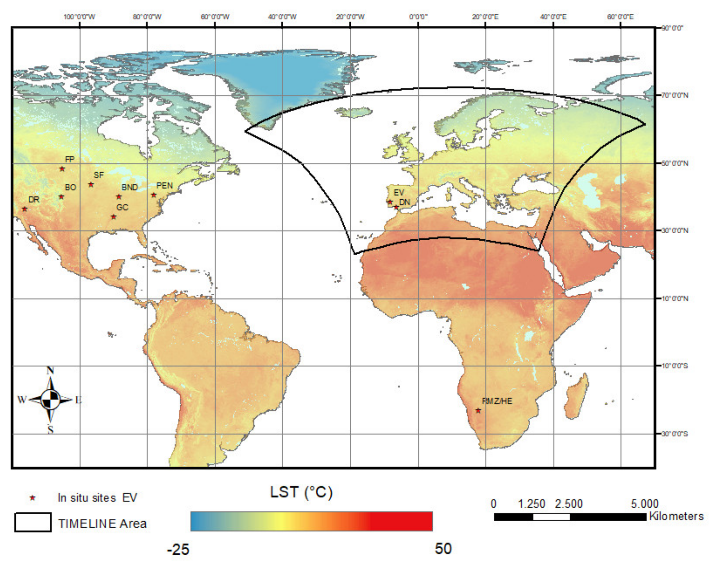
2.1. Study Area and Period

The area and period of the TIMELINE LST validation are determined by the study area of the TIMELINE project and the availability of in situ data. The validation between TIMELINE and MODIS LST was conducted for the years 2003 to 2014, where the most overlaps between TIMELINE and MODIS LST over the TIMELINE study area were found. Only in situ LST data from two sites in the TIMELINE study area were available for the period 2010–2013. Eight more stations were available in North America and South Africa (see Figure 2). Therefore, the validation of TIMELINE LST was extended to these regions for this period. The in situ measurement stations are described in Section 2.4.
The study area of the TIMELINE project is Europe and northern Africa, hawithving the same extent as the European Environmental Agency (EEA) reference grid: 900,000 m east, 900,000 m north to 7,400,000 m east, 5,500,000 m north. According to the Köppen–Geiger classification [49], Western Europe and the Mediterranean Basin have a temperate climate, with dry and hot summers in the Mediterranean regions (Csa) and warm summers in Western Europe (Cfb). Both European in situ sites, Évora (EV) and Doñana (DN), are situated in the Mediterranean Basin. Eastern and central Europe have a continental climate, with warm summers in central and central-eastern Europe (Dfb) and cold summers in Scandinavia and north-eastern Europe (Dfc). In northern Africa arid conditions with hot summers (Bwh) dominate.
The American in situ sites stretch over the whole United States; the most northern site is Fort Peck (FP) (48.3° N), the most southern site is Goodwin Creek (GC) (34.2° N), the most western site is Desert Rock (DR) (−116° E) and the most eastern site is located at Pennsylvania State University (PEN) (−77.9° E). According to the Köppen–Geiger classification, Bondville (BND), Boulder (BO), GC, PEN and Siuox Falls (SF) have a continental climate (Dfb, Dfa). GC has a temperate climate (Cfa), and Desert Rock (DR) is situated in a semi-arid region (BWk) [49]. The African sites Heimat/Rust mijn Ziel (HE) experience an arid, hot desert climate (Bsh), according to Köppen–Geiger classification [49]. The validation study is therefore representative of a wide range of climatic conditions.
The land cover in DR is defined as arid shrubland. BND and PEN are located in an agricultural area, and the land cover at these sites is cropland. The land cover at the remaining stations is grassland [15,42,50]. The measurement sites of BO, PEN and GC are relatively close to the forest edge, which is therefore also covered by the corresponding AVHRR pixels.

2.2. AVHRR LST

2.2.1. LST Derivation Algorithm

LST is retrieved from the brightness temperatures of cloud-free pixels over land using the TIMELINE Level 1B product, the Level 2 cloud mask, and the Level 2 water mask. When developing the TIMELINE LST processor, Frey et al. [4] analyzed the accuracy and error robustness of several split-window and mono-window algorithms for AVHRR data. They concluded that among the split-window algorithms, the algorithm by Becker and Li [5] is preferred, and the algorithm by Qin et al. [48] performed the best from the mono-window algorithms. Additionally, they developed the algorithm to make it applicable to all NOAA platforms in order to generate a consistent LST product for the whole AVHRR period. To enhance the error robustness of the algorithms, coefficients were added that should compensate for the impacts of TCWV, VA, and high LST values. A different set of coefficients is used for each sensor to consider the different spectral response curves of the NOAA sensors. Equation (1) shows the resulting split-window algorithm:
  α = 1 + p 1 1 ϵ ϵ + p 2 d ϵ ϵ 2 β = p 3 + p 4 1 ϵ ϵ + p 5 d ϵ ϵ 2 LST = p 0 + α t 4 t 5 2 + β t 4 t 5 2
where t4 and t5 are the brightness temperatures, ϵ is the mean emissivity of both TIR channels, dϵ is the emissivity difference in both TIR channels and p0p5 are the coefficients added by Frey et al. [4].
Equation (2) shows the resulting mono-window algorithm:
LST = 1 c ( p 2 1 c d + t 4 p 1 1 c d + c + d d T a t m ) c = ϵ τ d = 1 τ 1 + τ 1 ϵ τ = p 0 p 1 T C W V
where t4 is the brightness temperature, ϵ is the emissivity, T a t m is the mean atmospheric temperature, T C W V is the total columnar water vapor, and again p0p5 are the coefficients added by Frey et al. [4].

2.2.2. AVHRR Data

The AVHRR sensors on board the National Oceanic and Atmospheric Administration’s (NOAA) polar orbiting satellites (NOAA-1 to NOAA-19) as well as on the Metereological Operational (MetOp) satellites (MetOp-A, -B and -C) have delivered daily observations in visible, near-infrared, and thermal wavelengths from the early 1980s until today. Three different generations of AVHRR sensors have been developed over the past decades, providing observations in four, five, and six spectral channels, for each generation [44]. The resolution is around 1.1 km at the nadir, but this widens up to 6.5 km with the observation angle, which spans to a maximum of ±55.4 degrees.
LST is derived from AVHRR Level 1B data, which are calibrated, corrected for geolocation errors, and quality-checked. For LST over the TIMELINE study area, TIMELINE Level 1B data from the DIMS archive at DLR are used. The comprehensive preprocessing chain, which also comprises the calculation of the correspondent sun and satellite zenith angles, is described in [45]. For LST over North America and southern Africa, NOAA Level 1B data, which were downloaded from the NOAA Comprehensive Large Array Data Stewardship System (CLASS), are used. Their preprocessing, which also generates the correspondent sun and satellite zenith angles, is described in [51].

2.2.3. Auxiliary Data: TCWV, Tatm and Land Cover Data

TCWV (kg/m2) is defined as the total gaseous water contained in a vertical column of atmosphere. High TCWV levels often lead to a decrease in the accuracy of LST derived with split-window algorithms, because of the different and non-linear absorption properties of water vapor between two infrared channels [52]. In this work, TCWV data from the ERA-Interim Archive at the European Centre for Medium-Range Weather Forecasts (ECMWF) are used. The data comprise a meteorological reanalysis with a temporal resolution of 3 h and a spatial resolution of about 79 km [53]. For the derivation of TIMELINE LST, it is projected to the orbit of the respective input scene.
T a t m is a crucial parameter for the mono-window algorithm used by Qin et al. [48]. It is a proxy for the atmospheric upwelling radiance, which adds up to the land surface radiance received by the sensor. Frey et al. [4] derived T a t m by using the mean of all temperatures in the vertical column for each atmospheric profile from the atmospheric profile database Seebor 5.0 [54]. This definition of T a t m differs from the definition by [55], who defined T a t m as the temperature in the vertical column, integrated over the water vapor content at the different altitudes. However, the first validation results derived during the revision of the algorithm by Qin et al. [48] have shown that applying the definition of T a t m by [55] leads to substantially larger errors of TIMELINE LST, mainly at high temperatures and VAs. Therefore, it was decided to retain the definition of T a t m in [4].
To reduce the number of input datasets for operational LST processing, T a t m is proxied with the air temperature at a two-meter altitude ( T 2 m ). Using one half of the Seebor 5.0 dataset, Equation (3) was derived:
T a t m = 0.0017   T 2 m 2 + 1.21   T 2 m + 37.18
Using the other half of the Seebor 5.0 dataset, the modeled T a t m was compared to the real T a t m , leading to an r2 of 0.89. For the calculation of TIMELINE LST, T a t m is derived from the ERA 5 T 2 m dataset [56], which comprises reanalysis data with a temporal resolution of 3 h and a spatial resolution of about 31 km, using Equation (3).
As can be seen from Equations 1 and 2, the derivation of LST from TIR data is influenced by the emissivity of the surface. The emissivity is defined as the ratio between the TIR radiation emitted by the surface to the TIR radiation emitted by a black body. As the emissivity depends on the surface material and structure, it varies with land cover. The vegetation cover method by Caselles et al. [57] is used to estimate the emissivity. It combines spectral information about different land cover types with the seasonal fluctuation of vegetation cover, by estimating the fraction of vegetation cover (FVC) of each scene from the AVHRR reflective bands. The land cover type of each pixel is obtained from land cover classifications and assigned to an emissivity class. For the derivation of TIMELINE LST for the period from 2008, the GlobCover classification for 2009 [58] was used. For AVHRR 2 and 3 data from the years before 2008, the GlobCover classification for 2005 [59] was used. For AVHRR 1 data, the CCI classification for 1992 was used [60], adapting the vegetation cover method to the CCI classification system, as shown in Table S1.

2.2.4. LST Quality and Uncertainty

Additional to LST estimates, a quality and an uncertainty layer produced. The uncertainty value combines the uncertainty of the LST algorithm, the uncertainty from the emissivity estimation, the noise equivalent differential temperature and the uncertainty from geolocation. The uncertainty of the LST algorithm and the uncertainty from the emissivity estimation were simulated by [4]. For the noise equivalent differential temperature, a constant uncertainty of 0.12 K is assumed, derived from [61]. The uncertainty due to geolocation is the standard deviation of LST within an n × n window, with n either equal to 3, 5 or 7 depending on the quality of the Level 1B input data. The calibration uncertainty is simulated for an error of one percent in the brightness temperature. The uncertainties are combined with the following equation:
Unc = alg 2 + emi 2 + nedt 2 + geo 2 + cal 2
where alg is the uncertainty of the algorithm, emi is the uncertainty of emissivity, nedt is the noise equivalent differential temperature, geo is the uncertainty due to geolocation errors and cal is the calibration uncertainty.
The quality flags carry information about the quality of the emissivity estimation, the LST algorithm and the Level 1B input data. However, to assess TIMELINE LST for all land covers and climatic conditions, these flags were ignored.

2.2.5. Daytime Normalization

The assessment of the consistency of the whole TIMELINE LST time series is affected by the different observation times of the individual satellites, as well as by orbit drift, experienced by most of the NOAA satellites, leading to different observation times even within the time series of one satellite.
Daytime normalization can solve both problems. Daytime normalization is often performed by applying a diurnal temperature cycle (DTC) model. Göttsche and Olesen [62] proposed a DTC model developed for METEOSAT data. The daytime part of their model can be expressed as:
LST t = T 0 + T a cos π ω t t m
where T 0 is the LST at sunrise, T a is the temperature amplitude of the day, ω is the daytime length, t is the observation time and t m is the time of the maximum temperature. This model has already been used by Liu et al. [63] to normalize AVHRR LST to a certain observation time by transforming Equation (5) into the following equation:
LST t 1 = LST t 2 + T a cos π ω t 1 t m T a cos π ω t 2 t m
where t 1 and t 2 are two different times in the DTC model. The daytime length ω can be calculated via the geolocation and the day of the year. T 0 , T a , and t m are unknown in this study, and have to be modeled.

2.3. MODIS LST

In this study, the MYD11_L2 Collection-6 data [64] were used for comparison. The MODIS sensors, carried on the Terra and Aqua satellites, have provided daily data since the years 2000 (Terra) and 2002 (Aqua) with a spatial resolution of about 1 km at the nadir in the TIR channels 31 and 32. Each product contains LST from 5 minutes of MODIS acquisition. The MODIS Level 2 LST products are generated using the generalized split-window algorithm [11]. They are widely used and repeatedly validated [13,65]. The inputs for the algorithm are, besides the MODIS cloud and snow masks, the TIR bands from the radiance data product (MOD021KM), the water vapor data from MOD07_L2, and the MODIS land cover MCDLC1KM. Similar to the TIMELINE LST algorithm, the generalized split-window algorithm uses different coefficients for day- and nighttime LST. Atmospheric corrections were obtained from MODTRAN 4 simulations. View angle errors are corrected with a quadratic term of the difference between brightness temperatures in the thermal bands. Emissivity is calculated via the classification-based method by [66]. This method provides emissivity values for various land cover classes, which are identified based on land cover type and seasonal dynamic, also taking into account angular effects through a bidirectional reflectance distribution function model.
Quality flags for every pixel are calculated during the production. The 16-bit flags contain information about the quality of the input data, cloud contamination, the quality of the emissivity and the quality of the split-window algorithm application [67].

2.4. In Situ LST

In situ radiometers and the AVHRR sensor measure on totally different spatial scales. Therefore, in situ measurement sites have to be representative for the surrounding pixel area, and have to be in an homogeneous environment [15]. Only a few TIR measurement stations exist that match these criteria. Ten measurement sites have been chosen, located in Europe (EV and DN), southern Africa (HE), and North America (seven surface radiation network (SURFRAD) stations). As only in situ data for the years 2010 and 2013 are available for HE, the investigation period of the validation with in situ data is 2010–2013. Table 1 provides an overview of the used validation data, while Figure 3 shows the surroundings of the sites on the AVHRR scale.
The measurement settings and calculation of the in situ LST for HE are described in [15]. The measurement settings and calculation of the in situ LST for EV are described in [68]. The in situ LST for DN was measured and calculated as described in [50]. SURFRAD radiometer measurements were conducted as described in [42], and were processed into LST using the Stefan–Boltzmann law. The surface emissivity at the SURFRAD sites has been derived via the broadband emissivity method, as suggested by [69], based on the global 5 km monthly MODIS LST/emissivity product MOD11C3 [70].

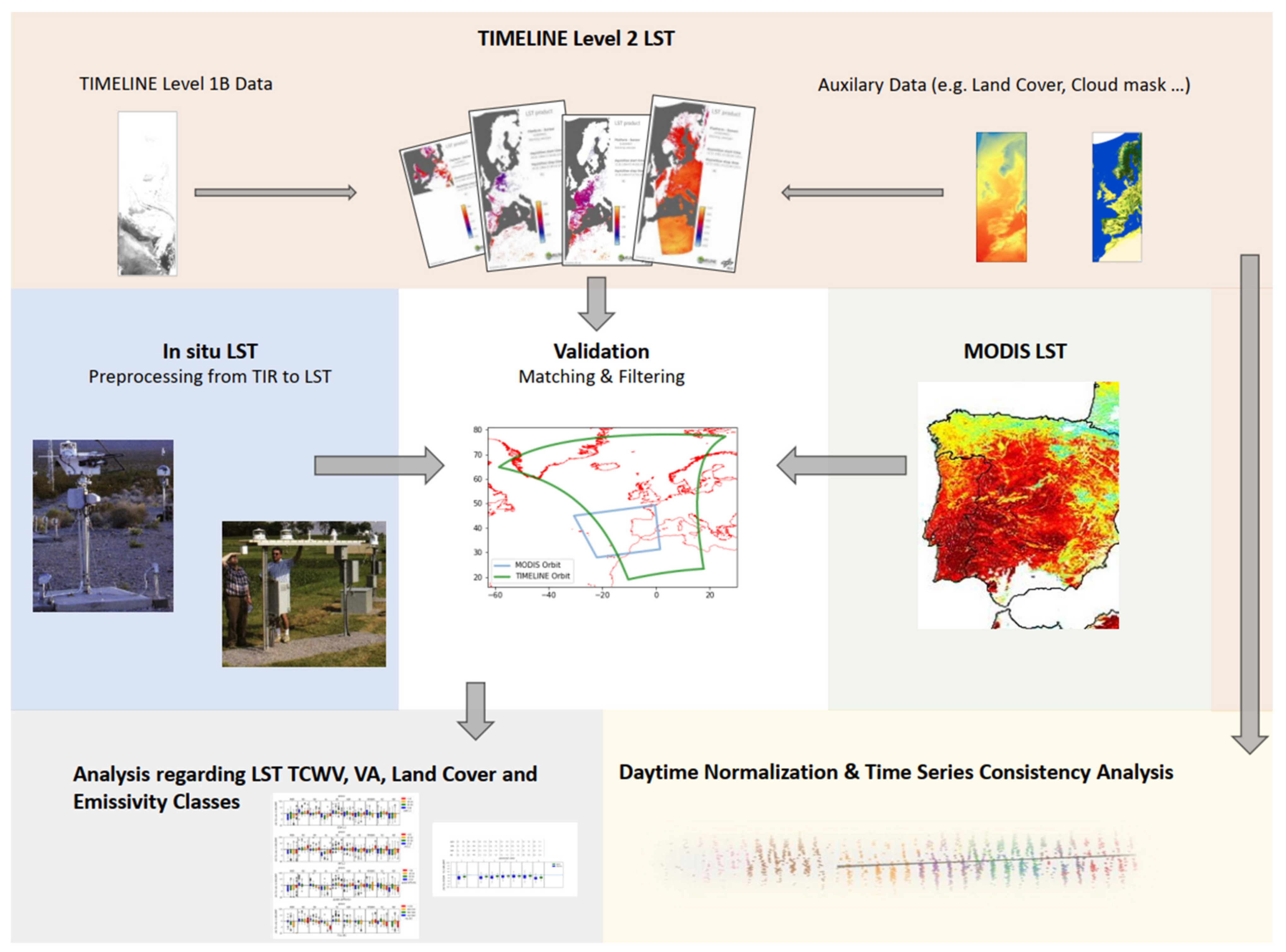
2.5. Validation Approach

The validation approach consists of the following aspects.
(a) Inter-comparison between AVHRR LST and in situ LST obtained at 10 stations located in Europe, North America and southern Africa. The in situ measurements at DN were performed every 10 s, but the final value was stored as a 5 min average. At the other stations, the measurements have a temporal resolution of one minute. All in situ measurements were filtered using the quality flags, generated by the respective data provider. The AVHRR LST was filtered using the quality flags from the Level-1B input data and with the uncertainty value (<2 K), which was generated during the TIMELINE LST production. For comparison, the average LST in a window of three by three pixels over the station was calculated, but only if all values in that window were valid and only if the standard deviation in this window was less than 1 K. This was to ensure a valid match between the in situ point measurement and the averaged raster data. On the one hand, this takes account of possible geolocation errors, which are common in AVHRR data. On the other hand, cloud borders are filtered out, which were responsible for most of the outliers. In total, 2402 individual in situ measurements were compared to the AVHRR LST.
(b) Comparison of the AVHRR LST product with concurrent MODIS LST (MYD11_L2 product) [64]. The comparisons were conducted over the TIMELINE study area and limited by the MODIS lifetime to the years 2003–2014. Again, only MODIS LST and AVHRR LST with good quality input data and an uncertainty smaller than 2 K were compared. The uncertainty threshold is a compromise, ensuring the high quality of LST, but also keeping enough data points for the validation. Only pixels satisfying the following criteria were selected: the VA is not more than 40°, the VA difference between AVHRR and MODIS is not more than 20°, and the maximum sun zenith angle (SZA) is 90°. The maximum slope allowed was 10° using the 1 km slope GMTEDmd dataset [71]. A maximum time difference of 10 minutes between AVHRR and MODIS acquisitions was permitted, as suggested in [10]. Differences greater than 10 K were filtered out as outliers. After applying the previously mentioned filters, these made up 0.2% of the data points. To reduce the total number of scene comparisons, only AVHRR/MODIS pairs with more than 100,000 valid observations were selected. In total, 905 MODIS scenes were compared to the AVHRR LST, resulting in more than 187,000,000 data points.
(c) Since LST is derived from the TIR radiation emitted by the surface, as seen within the sensor field of view, it is a directional variable [72]. As a directional variable, it is strongly affected by differences in viewing and illumination geometry [73]. As already mentioned, the estimation of LST is influenced by the atmosphere and the emissivity of the surface. To better quantify these influences on the achieved LST accuracy and therefore identify reliable LST ranges and acquisition conditions, all validation results were investigated for different VA and LST classes, as well as regarding different land cover types and TCWV classes.
(d) In order to use the AVHRR LST time series as long-term measurements, the consistency between the different AVHRR sensors has to be assessed. The validation with in situ and MODIS LST covers the period from 2003 to 2014, and thus only parts of the multi-decadal time series and only the later NOAA missions. The comparison to other LST data sources at earlier parts of the time series is not possible as AVHRR was the only high-temporal frequency remote sensing acquisition system, and measurement sites suitable for the validation of remotely sensed LST did not exist. Therefore, a time series analysis of TIMELINE LST at three sites was conducted. The whole time series over the in situ sites DN and EV and the pseudo-invariant calibration site Algeria3 (Lat:30.185/Lon:7.59) was extracted for detailed analysis. Algeria3 was chosen because it is recommended by the CEOS/WGCV/IVOS subgroup for its temporal stability and spatial homogeneity [74]. Due to its arid conditions, only minor cloud contamination is expected, and it is a desert site, meaning variation due to vegetation or soil moisture is minimal. According to Jin and Treadon [75], the diurnal LST cycle depends on geolocation, soil or vegetation properties, and season. To reflect its seasonal variability, the parameters of the DTC model were derived for each month separately. The relatively low monthly resolution was chosen to account for the limited amount of data points in the time series. The DTC parameters were derived using the following procedure: One half of the respective time series was selected using the numpy random choice method [76]. These training samples were then aggregated for every month. For each month, LSTs from almost every NOAA platform were available, which covered large sections of the respective DTCs. For these monthly aggregated LSTs, the parameters of the DTC model described in 2.2.5 were determined by fitting Equation (5) via least squares to the data. Figures S1–S3 show the monthly aggregated LSTs and the resulting monthly DTCs for each site. Only data points before 18 h true solar time were used, so that the attenuation effect of the LST cooling in the evening [62] can be neglected. The other half of the LSTs was used to estimate the monthly error associated with the DTC modeling. To improve the temporal resolution of the parameters, they were linearly interpolated to every day of the year. Equation (6) was then used to normalize the TIMELINE LST time series at all three sites to 14.30 h true solar time. At days on which LSTs from multiple NOAA sensors were recorded, a cross-sensor comparison was conducted.
(e) For characterizing the differences, several validation metrics were used: the root mean square error (RMSE), the mean absolute deviation (MAD), the mean deviation (MD) and the standard deviation of the error (σ). While RMSE and MAD measure the magnitude of the error, MD indicates the direction of the error, often referred to as bias. σ measures the dispersion of the error and is therefore an indicator for the precision. Although RMSE and MAD are quite similar metrics, both were investigated to make this study comparable to studies that use either one.

3. Results

3.1. Assessment of the TIMELINE LST Accuracy

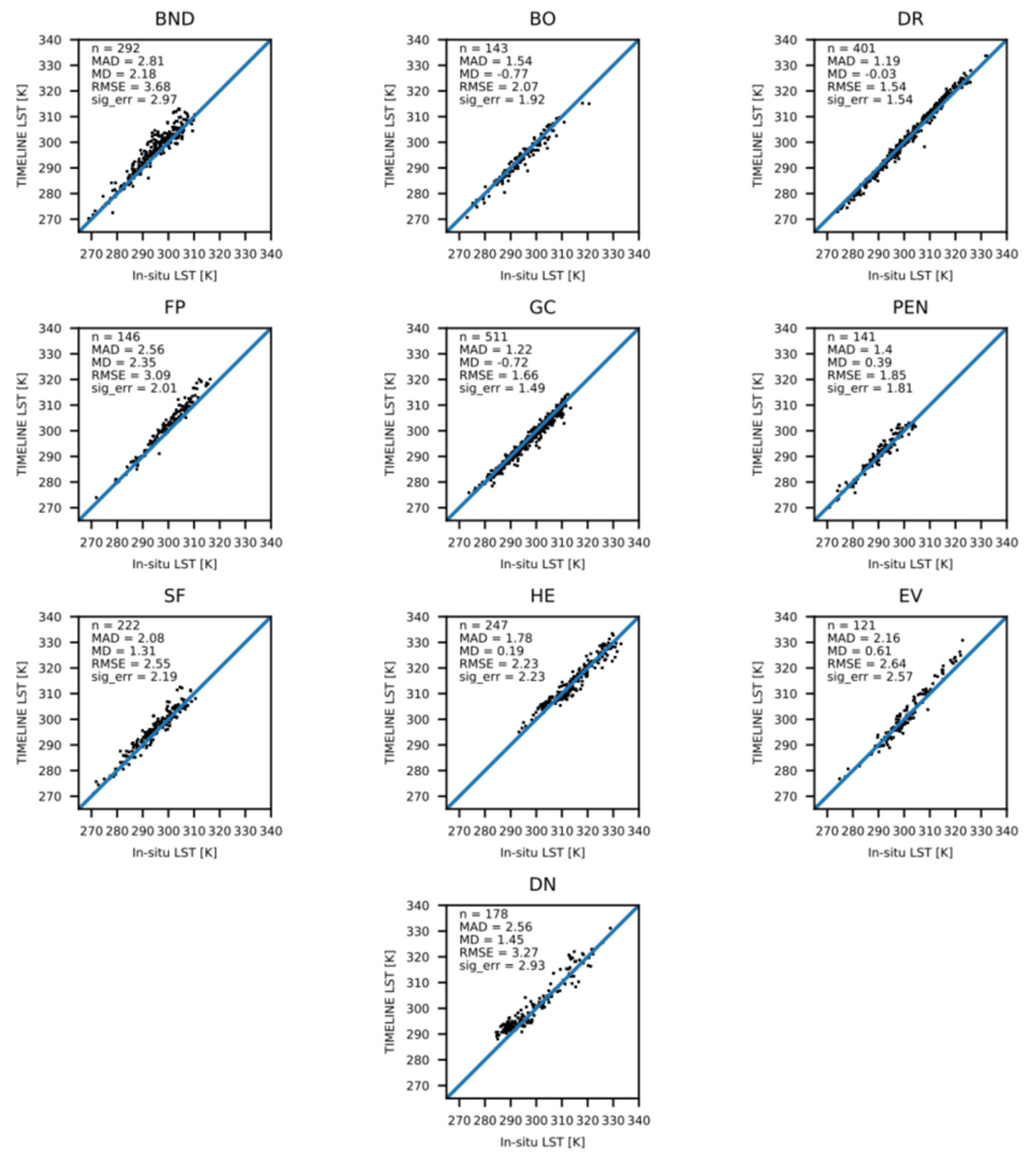
3.1.1. Comparison to In Situ LST

The comparison with in situ LST comprises TIMELINE LST from the years 2010–2013 derived from NOAA-15, 16, 18 and 19 data. Figure 4 shows TIMELINE LST plotted against in situ LST at the 10 stations. The sites with the most data points are GC and DR. The sites with the fewest data points are EV, for which only in situ data for 2010 were available, as well as FP, PEN and BO. The overall MAD is 1.8 K, the MD is 0.5 K, the RMSE is 2.43 K and σ is 2.38 K. A seasonal pattern is visible: In summer (April–September), the agreement is lower, with a MAD of 2.07 K, an MD of 0.88 K, an RMSE of 2.71 K and a σ of 2.57 K. In winter (October–March), the MAD is 1.54 K, the MD is 0.14 K, the RMSE is 2.12 K and σ is 2.12 K.
The highest agreement was reached at DR and GC. The lowest agreement was found at BND. Clear positive MDs were observed at FP, BND, DN and SF. Light positive MDs were observed at EV, PEN and HE, and a fairly balanced MD at DR. Light negative MDs were observed at GC and BO. Figure 4 shows a considerable positive MD of TIMELINE LST at BND, FP and EV at LSTs over 300 K.

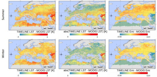
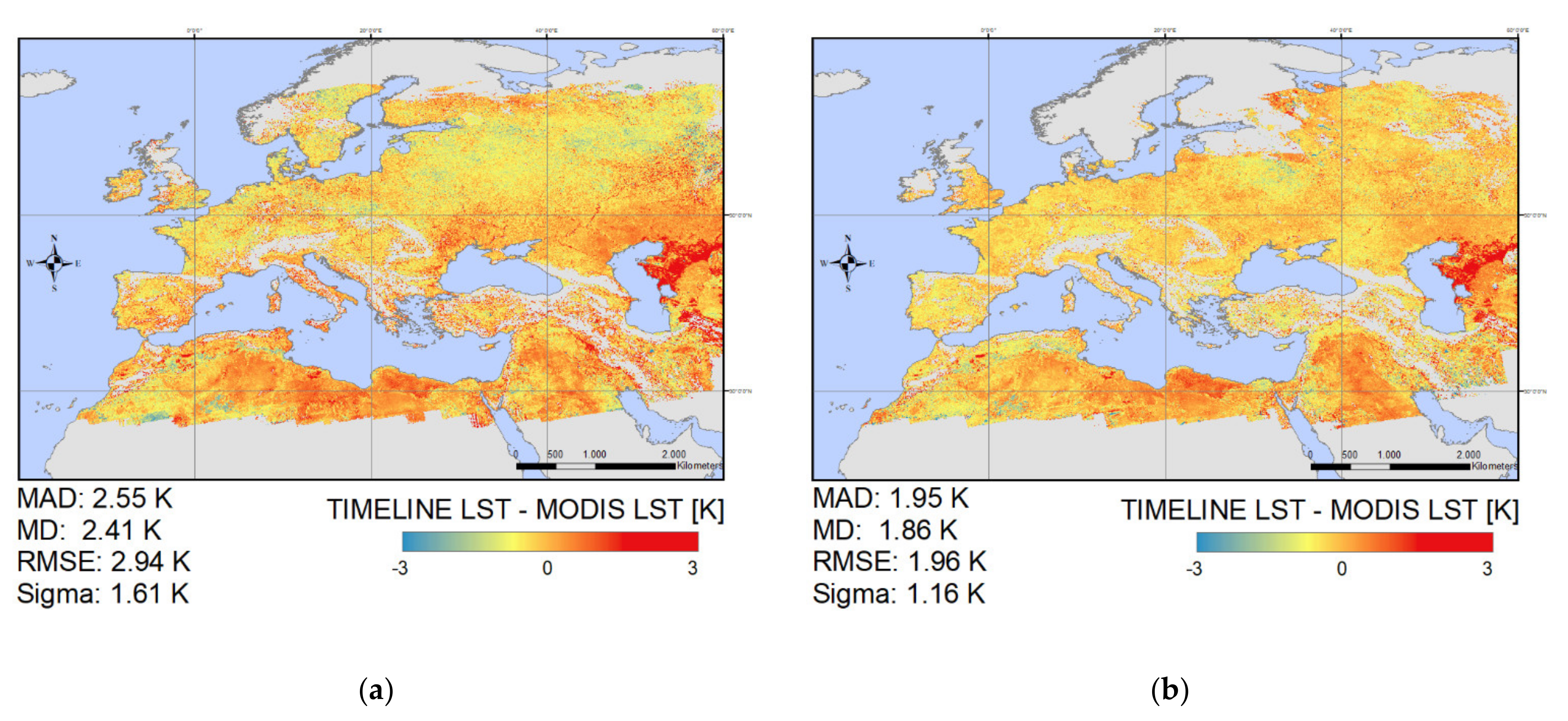
3.1.2. Comparison to MODIS LST

The comparison between TIMELINE and MODIS LST was conducted for 905 spatial and temporal matches of MODIS and AVHRR scenes. The scenes were filtered as described in 2.5 The comparison was done for the years 2003–2014 over the TIMELINE study area for scenes from NOAA-16, 18 and 19. The map in Figure 5 shows the count of the observed matches between TIMELINE and MODIS LST per pixel. The observed data points extend over the whole TIMELINE study area, between 20° and 60° N, and −20° and 60° E. Most observations were found around the Mediterranean Sea between 30° and 45° N. Therefore, arid areas are overrepresented. Mountain areas are not covered due to their high slopes. Regions north of 60° N are not covered because of low sun angles. The maximum count is 99 observations per pixel.
Figure 6 shows boxplots for the difference between TIMELINE and MODIS LST for each overlap. The plot reveals a general positive bias of TIMELINE LST towards MODIS LST. It shows the seasonal pattern, with lower accordance and higher bias in summer and higher accordance and lower bias in winter. This is supported by the substantially lower RMSE, MAD, MD and σ in winter, as displayed in Figure 7b. Figure 7a–c show the spatial distribution of the difference between TIMELINE and MODIS LST. Generally, the difference increases from north to south, i.e., with higher temperatures. TIMELINE LST is especially higher than MODIS LST in the desert regions of northern Africa and east of the Caspian Sea. As visible in Figure 7a, in summer, the positive bias of TIMELINE LST can also be observed in the steppe and agricultural areas of west, middle and Eastern Europe. Figure 7c shows that the lowest error is found in the deciduous and evergreen forests of central Europe and the boreal forests of northern Europe. Some spatial patterns of the LST difference show direct links to the observed emissivity difference, displayed in Figure 7d. For example, the desert regions in northern Africa and east of Caspian Sea, where a high emissivity and LST difference can be observed. In general, the TIMELINE emissivity is lower than the MODIS emissivity. However, this applies especially to the bare ground areas. Over the boreal forest of Siberia, the emissivity difference is quite low, leading to substantially lower MDs in these regions.

3.2. Robustness of the LST Derivation Approach

In the following subchapters the difference between TIMELINE LST and in situ and MODIS LST is analyzed concerning the influencing factors TCWV content, LST level, VA, emissivity and land cover. The influence of the LST and TCWV level on the LST accuracy has been determined in several studies, e.g., [9,52]. Directional effects represented by the VA are described in [4,73,77,78]. The emissivity and land cover are important factors in the LST estimation, which have to be known a priori. For the analysis, the matches between TIMELINE LST and the validation LST were classified for the respective variable. The classes reflect the range and distribution of the respective variable. The boxplots in Figure 8 and Figure 9 show the behavior of the difference for each class. To get a more isolated picture of the impact of the respective variable on the error, the matches with values in the highest classes of the other influencing variables have been filtered out. For example, in Figure 8b and Figure 9b, only matches with an LST smaller than 315 K and a VA smaller than 50° were used. The boxplots in Figures S5, S6 and Figure 10 show the difference between TIMELINE and MODIS LST for each emissivity class classified for LST, VA and VA difference between AVHRR and MODIS, and for summer and winter. Only the difference between TIMELINE and MODIS LST from 2013 was analyzed in the following. Figure S4 shows TIMELINE LST against MODIS LST in 2013. It shows a very high accordance with an r-value of 0.99, but also the tendency of TIMELINE LST to overestimate at higher LST levels.

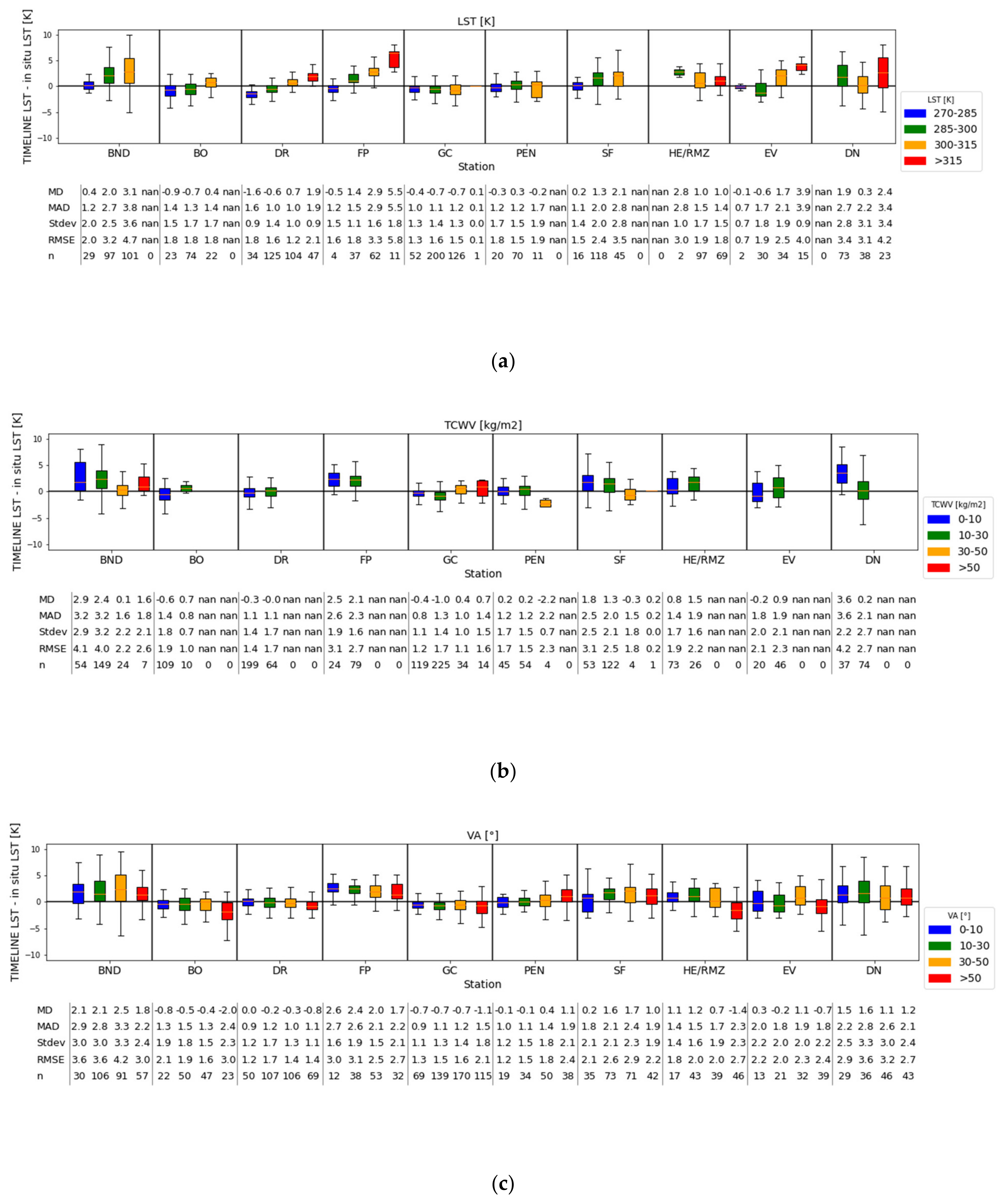
3.2.1. Robustness to Variances in LST, TCWV, and VA

The comparisons to MODIS LST and to in situ LST show a higher MAD, RMSE, MD and σ with increasing LST level. As is visible in Figure 8a, high MADs, RMSEs and σ occur at high LST levels at BND, DR, FP and EV. While the MD is stable over the LST levels at GC, PEN and DN, there is a strong positive connection between the LST level and MD visible at BND, BO, SF, FP, EV and DR. Notable high errors occur at LSTs over 315 K. Figure 8b shows no systematic impact of TCWV on the difference between TIMELINE and in situ LST. At BND, PEN and SF, the MD drops at TCWV levels over 30 kg/m2. At BO, DR, FP, HE, EV and DN, high TCWV levels only occur at high LST levels, and have therefore been filtered out. Figure 8c shows directional effects at HE, EV and BO, especially at VAs higher than 50°, with considerably lower MDs at these angles. This effect is more moderate at DR, GC, FP and DN. Because of the positive bias of TIMELINE LST at DN and FP, these sites experience a lower MAD and RMSE at higher VAs. At BND and SF, no systematic impact of the VA is visible. At PEN, there is a positive connection between the VA level and the MD.
In Figure 9a, a clear positive relationship between the difference between TIMELINE and MODIS LST and the LST level can be observed. As with the comparison with in situ LST, MAD, RMSE, MD and σ increase with higher LST levels. Figure S5 shows that this relation is valid for all emissivity classes except class 8 (bare ground), which shows high errors and a high bias at all LST levels. Class 2 is an exception because of known errors during the TIMELINE emissivity estimation. Figure 9b shows a weak positive relationship between the TIMELINE and MODIS LST difference and TCWV. Figure 9c shows almost no relationship between the sensor angle and the difference between TIMELINE and MODIS LST. Figure S6 shows that MAD, RMSE, MD and σ are stable for different VAs and VA differences at all emissivity classes, even at classes with a complex surface, such as forests and shrublands.

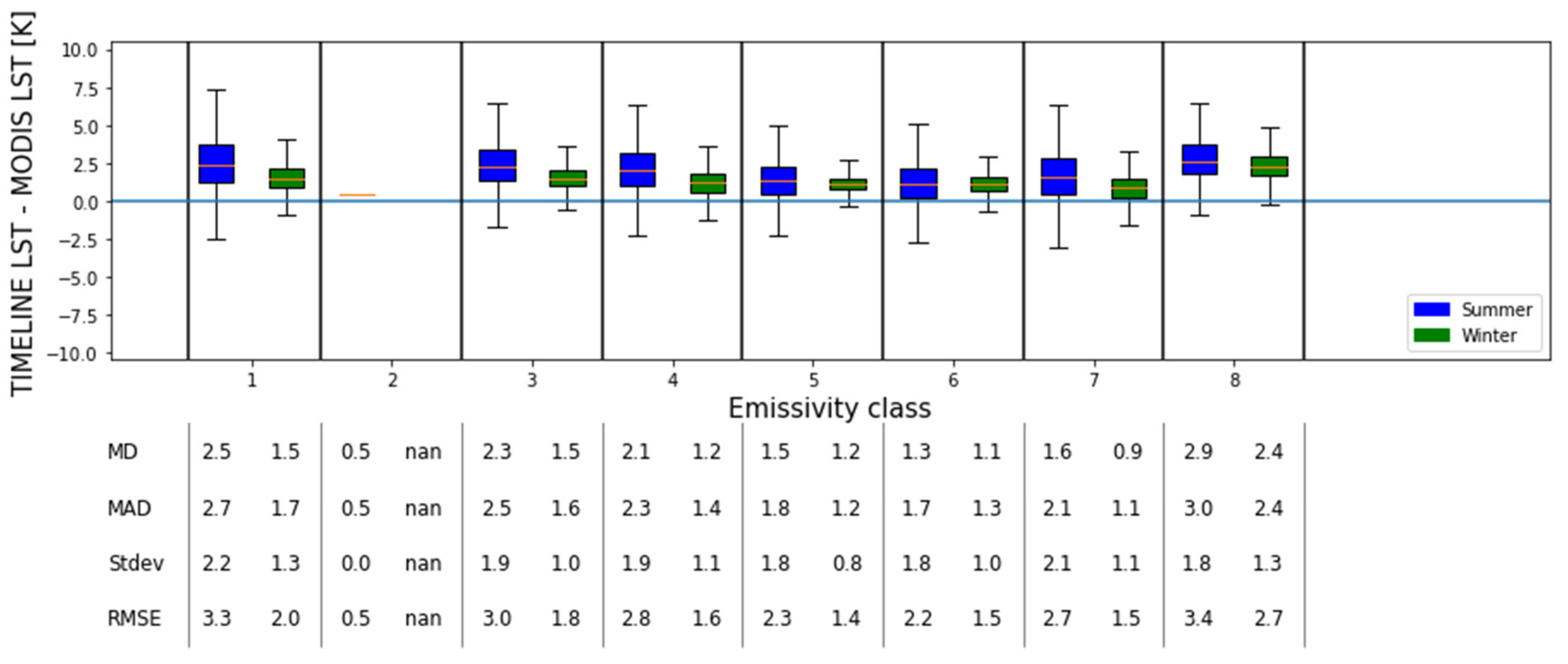
3.2.2. Land Cover and Emissivity

As mentioned in Section 2, the emissivity for the TIMELINE LST product is derived from the vegetation cover method [57], while the emissivity for the MODIS LST product and in situ LST is derived from the classification-based method created by [66]. Figure 7d shows that the different methods can lead to absolute differences in emissivity up to 0.04. An especially high difference can be seen in the arid regions with bare ground. Smaller seasonal differences are experienced within the vegetation classes.
Figure 9d shows the strong negative dependence of the differences between TIMELINE and MODIS LST and their corresponding emissivity differences, which can be justified by the split-window algorithm: an underestimation of the emissivity automatically leads to an overestimation of LST. Figure 9d shows that the MD for LSTs calculated with an emissivity difference between −0.06 and −0.03 is about 4.4 K, while the MD for LSTs calculated with no emissivity difference is about 1.7 K. Figure 10 shows that MAD, RMSE, MD and σ are higher in summer than in winter for all emissivity classes. The lowest accordance is found with class 8, with a MAD and MD of almost 3 K in summer and around 2.3 K in winter. The best accordance is reached in both forest classes 5 and 6, with MADs of 1.59 K and 1.7 K and MDs of 1.35 K and 1.39 K in summer, and MADs of 1.35 K and 1.41 K and MDs of 1.25 and 1.26 K in winter. It is notable that these classes show the highest seasonal stability. High seasonal differences can be seen for the classes 1, 3, 4 and 7. Figure S7 illustrates the difference between the MODIS emissivity used for the in situ LST calculation at the SURFRAD sites and the TIMELINE emissivity. The stable pattern of the MODIS emissivity is created by the method derived from [66], for which—contrary to the vegetation cover method—vegetation indices are not part of the emissivity derivation formula, but only used to distinguish emissivity classes. However, the absolute difference is very small in the vegetation classes (<0.01). To estimate the propotion of the error between TIMELINE and in situ LST due to the emissivity difference between TIMELINE and MODIS emissvity, in situ LST at the SURFRAD stations was recalculated with TIMELINE emissivity. However, using the alternative procedure would not have led to significantly different results, as displayed in Figure S8. The MAD between TIMELINE and in situ LST would only have changed in the order of 0.04 K.

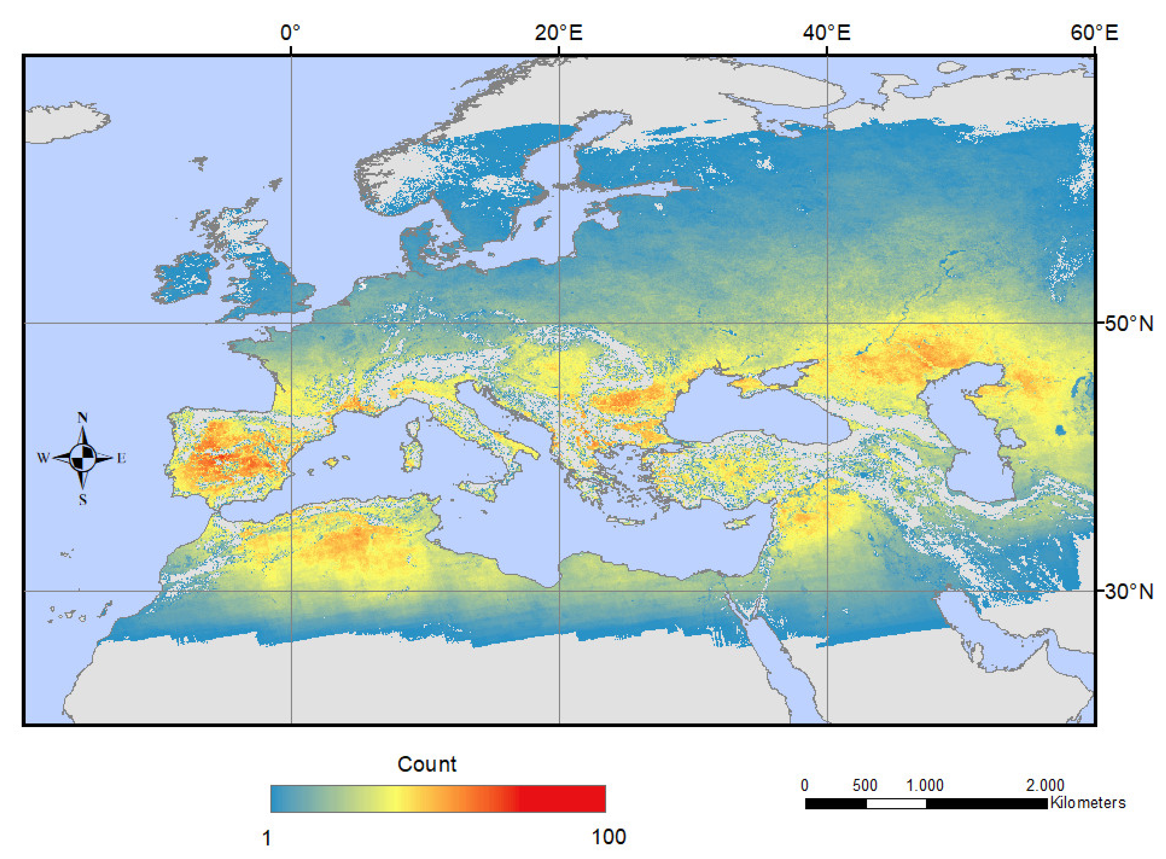
3.3. Assessment of the TIMELINE LST Consistency

Figure 11 shows the parameters of the DTC models for Algeria3, DN and EV. As expected, the seasonal development of most of the parameters at DN and EV is quite similar because of their geograpical proximity and the similar land cover at these sites. The T 0 (LST at sunrise) is around 280 K at all three sites in winter, which rises to 300 K at Algeria3 and 290 K at DN and EV in summer. The temperature amplitude T a increases from 10 K in winter to 30 K in summer at EV and DN, and from 20 K in winter to 30 K in summer at Algeria3. t m (time of maximum temperature) shows no seasonal pattern, varying around 13 h true solar time. The highest fluctuations at DN are between 13.30 h in February and 12.30 h in the second half of the year. The DTC models show their highest uncertainties in spring and autumn, with RMSEs up to 4.5 K. Lower RMSEs between 2.5 and 3 K are recorded in the winter and summer months.
Figure 12 shows the original TIMELINE LST time series at Algeria3, EV and DN. Figure 13 shows these time series normalized to 14.30 h true solar time with Equation (6) and the parameters of Figure 11. It is visible that the across-platform offsets and the orbit drift effects are successfully minimized in the time series. The LST values from NOAA-10, which have been calculated with the mono-window algorithm constructed by [48], fit consistently into the time series. The LST values from the other platforms were calculated with the split-window algorithm devised by [4].
The LST normalized to 14:30 allows cross-sensor comparisons at days when LST values from multiple platforms were recorded. Figure 14 shows these comparisons for NOAA-9, 10, 11, 12, 14, 15, 16, 17, 18 and 19. The highest accordance is achieved between NOAA-18 and 19, with an RMSE of 1.72 K, and a mean observation time difference of 0.74 h. The lowest accordance is reached between NOAA-16 and NOAA-15, with an RMSE of 5.39 K, and a mean observation time difference of 6.12 h. The errors show a positive connection to the observation time difference. A mean RMSE of 2.38 K is found. The cross-sensor comparison also reveals some systematic errors: TIMELINE LST from NOAA-16 shows a positive MD towards LST from NOAA-12, 14, 15 and 17 at temperatures over 320 K, which are mainly found at Algeria3. Additionally, NOAA-11 shows a positive MD in comparison to NOAA-10 and 12 of 2.4 K.

4. Discussion

4.1. TIMELINE LST Accuracy

4.1.1. Comparison between TIMELINE LST and In Situ LST

Considering the previous accuracy analysis of TIMELINE LST by [4], the error lies in the expected range of 1–3 K. Similar accuracies were reached in a recent study by [79], comparing a global 0.05° × 0.05° AVHRR LST product to in situ LST from SURFRAD sites, resulting in RMSEs between 2.25 K and 3.86 K. In studies for different sensors, errors of this range are common, for example: the LST from MODIS data was derived with an average RMSE of 2.65 K compared to in situ measurements by [12], or compared to modeled brightness temperatures with less than 1 K on average by [13]. The LST product for SERVIRI was validated with in situ data from the Karlsruhe Institute of Technology (KIT), resulting in RMSEs between 1.2 and 4.1 K [15]. LST from AASTR was derived with an average RMSE of 3.03 K in comparison with in situ measurements [19].
The MADs at the in situ sites partly reflect their homogeneity at the AVHRR pixel scale, which is illustrated in Figure 3: DR, which is surrounded by arid shrublands, has the lowest MAD, while BND, which is surrounded by a mix of grassland, cropland and trees, has the highest MAD. Ma et al. [79] and Martin et al. [77] observed large differences between the growing and dormancy season around the BND site, leading to high errors during the comparison with remote sensing LST at this site. A negative bias at BO and GC was also observed by [79]. This can be explained by the presence of forest and vegetation near the measurement site, which is in the AVHRR field of view.

4.1.2. Comparison between TIMELINE LST and MODIS LST

The comparison between TIMELINE and MODIS LST resulted in a MAD of 2.34 K, an RMSE of 2.67 K and an MD of 2.21 K. This compares with a relatively small σ of 1.45 K, which indicates a systematic positive bias of TIMELINE LST towards MODIS LST. The previous studies comparing AVHRR LST to MODIS LST resulted in slightly better results, with MADs < 2 K in [4] and an overall MAD of 2.2 K in [78]. However, the observed number of data points by [4] was far smaller, and Frey et al. [78] applied stricter filtering before the validation (maximum observation time difference of 5 minutes, only one land cover in 5 × 5 pixel window, slope < 2°). The less strict criteria in our study were chosen in order to achieve a higher general validity.
According to [78], the factors that lead to different LST estimations between LST remote sensing products in general can be divided into two groups. The first group comprises differences in the acquisition conditions, such as observation time or view angle. These factors should be filtered out before the validation. The second group contains differences in the quality of the instruments and differences of the algorithms: this includes the sensor calibration and atmospheric correction, which is, in the case of the MODIS and TIMELINE LST product, the split-window or mono-window algorithm, respectively. Furthermore, it includes cloud detection and emissivity estimation.
As probable factors explaining the positive bias of TIMELINE LST, inconsistencies over the LST range were identified. The reasons for this will be further assessed in future versions of the product. On the other hand, a strong negative relationship between the differences in LST and the differences in emissivity were identified. The reasons for this bias lie in the emissivity algorithms and the respective assumptions about the land cover. Another factor could be the tendency of the MODIS LST product to generally underestimate LST. This is indicated by the study [12], who observed an MD of −0.93 K when comparing ten years of Collection 5 Aqua/MODIS LST to in situ measurements. For Collection 6, the MODIS LST product was improved mainly over bare soil. The validation of Collection 6 MODIS LST over the SURFRAD sites and EV conducted by [14] for the years 2004 and 2005 showed that, for most stations, the MD is still negative. The direct comparison at the respective sites in Table 2 shows that, except for BO, the MD between TIMELINE and in situ LST is around 2 K higher than the MD between MODIS and in situ LST. This fits very well with the observed positive MD between TIMELINE and MODIS LST in the emissivity class 3 (croplands and grasslands, see Figure 10), which is also in the order of 2 K. Despite the fact that the MODIS LST product experiences the same uncertainties as every remote sensing LST product, because of its long history of development and validation, it is expected to produce a very high quality of LST.

4.2. Robustness of the LST Derivation Approach

4.2.1. Robustness to Variances in LST, TCWV and VA

One aim of the TIMELINE LST algorithms is to minimize the LST error due to LST level, TCWV and VA. During the assessment of the revised algorithms by [4], some differences regarding these variables were still observed. For the split-window algorithm, the MAD was 0.7 K higher at the TCWV level of 50 kg/m2 than at 10 kg/m2. Especially, at high TCWV levels in combination with high Vas, high MADs occurred. Contrary to our results, the MAD over different LST levels was quite stable.
At least for the validation with MODIS LST, the LST level seems to be a determining factor in the resulting error and uncertainty (MAD at >315 K is 1.7 K higher than at 270–285 K). Some in situ site-dependent effects could be explained by seasonal differences in land cover, e.g., at BND. Leaving this special case aside, the higher uncertainties and errors at high LSTs seen in both validations are probably the reason for the seasonal pattern of the differences. The tendency for higher errors with higher LST levels and a positive bias of split-window algorithms for AVHHR is well known, and has been observed, among others, by [4,9]. This behavior was not observed during the evaluation of the split-window algorithm for MODIS LST [12,13,80]. The reasons for the remaining inconsistency over the LST range possibly lie in the coefficient retrieval process, specifically in the underlying Seebor database.
The comparison with MODIS LST showed only a weak positive dependence of MAD, RMSE, MD and σ on TCWV levels (the MAD at 30–50 kg/m2 is only 0.4 K higher than at 0–10 kg/m2). The split-window algorithms for TIMELINE and for MODIS LST apply different coefficients depending on the TCWV levels. This similar approach may also be the reason why TCWV content has only a weak impact on the difference between TIMELINE and MODIS LST. The comparison with in situ LST showed site-dependent behavior. Noticeable is the drop in the MD at BND, PEN and SF, which is still to be examined. At sites with warmer and more arid climates (BO, DR, FP, HE, EV and DN), the TCWV level is connected to the LST level, which makes an isolated analysis of the impact of these variables challenging. The Era Interim TCWV product has a resolution of 79 km, which may lead to inaccuracies in TCWV on the AVHRR scale. However, the sensitivity analysis by [4] showed that only TCWV errors in the order of 15 kg/m2 have an impact on the LST error. This variance in TCWV is not common at the 79 km scale. Therefore, an impact of the different spatial scales of the TCWV and AVHRR data on the LST error is not expected.
Frey et al. [78] stressed that allowing higher sensor view angles and view angle differences leads to a visible increase in difference between AVHRR and MODIS LST. Therefore, the comparison between TIMELINE and MODIS LST was only conducted over a quite narrow range of VAs (0–40°) and VA differences (0–20°). The difference between TIMELINE and MODIS LST showed a high stability over these ranges for all emissivity classes. The comparison with in situ LST showed medium directional effects at HE, EV and BO, and light directional effects at DN and FP. The highest impact was visible at VAs over 50°. Martin et al. [77] observed similar effects at EV, which are explained by tree shadows at this site. Furthermore, they observed directional effects at BO and DR because of the high slopes around the site, and at FP, GC and DN because of vegetation. Ermida et al. [73] stated that viewing geometry effects have the greatest impacts on surfaces with high contrasts in the temperatures of the various surface elements, such as savanna-like landscapes, which applies to HE, DN and EV. The surprising positive connection between the VA level and the MD at PEN is still to be examined.

4.2.2. Land Surface Emissivity

The vegetation cover method was developed for the AATSR 11 μm and 12 μm bands, which have a similar measurement spectrum as the AVHRR thermal bands (10.3–11.3 μm, 11.5–12.5 μm). The method by [66] was developed for the MODIS thermal bands 31 and 32, which have a similar but narrower measurement spectrum (10.8–11.3 μm, 11.8–12.3 μm). Both the vegetation cover method devised by [57] and the method by [66] define emissivity values based on spectral measurements conducted for the vegetation and ground portion of the respective land cover class. However, while the formula devised by [57] integrates the seasonal variation in vegetation through the FVC, the method by [66] uses a priori information about the seasonal variation to distinguish emissivity classes. Directional effects on emissivity are only considered by [66].
The analysis showed a high impact of the emissivity difference on the difference between TIMELINE and MODIS LST. Frey et al. [4] analyzed the sensitivity of the Becker and Li split-window algorithm to emissivity, and observed that a deviation of 0.015 can lead to LST deviations of more than 1 K. This result can be confirmed by our study.
The emissivity estimated for TIMELINE LST is generally lower than the emissivity for MODIS LST. However, the difference is especially extreme in the emissivity class 8 (bare rock), which has the lowest emissivity level, whereas in the forest classes 5 and 6, the TIMELINE emissivity in summer is even higher than MODIS emissivity. This leads on the one hand to a strong positive MD and high MAD in arid regions, and on the other hand to a quite balanced MD and a low MAD over the forests of central and north Europe. Frey et al. [78] assumed an overestimation of emissivity by the MODIS product in these regions. Wan et al. [13] observed a serious underestimation of LST by the previous version of the MODIS LST product over arid regions, which led to further refinements in the split-window algorithm and emissivity estimation, resulting in an emissivity increase. Besides the dependence of the error on the LST level, the emissivity difference is the main driver of the distinct spatial distribution of the error, with low errors in the north of the TIMELINE study area and higher errors in the south.
Caselles et al. [57] based their method on measurements from the ASTER spectral library [81], while [66] based their method on measurements by [82]. The results for the respective emissivity class are quite different: according to [57], the mean emissivity in both TIR bands of class 8 is 0.94, while according to [66] it is 0.969. Smaller differences can be found in other classes. These differences have a direct impact on the LST differences of the two datasets. This illustrates the problem that emissivity can hardly be measured directly from space, but is a very sensitive input parameter for the split-window algorithms.
Besides the different methods of emissivity estimation, the different input datasets used for the estimation should be noted. While the MODIS emissivity algorithm uses the daily land cover information of the MCDLC1KM product, TIMELINE LST uses land cover classifications from 1992, 2005 and 2009. In return, the FVC, as part of the vegetation cover method, provides land cover information for the respective AVHRR scene. In addition, there are different spatial scales of AVHRR and MODIS. For the validation with in situ LST, the LST error caused by emissivity difference is superimposed by different LSTs within the AVHRR pixel.

4.3. Time Series Consistency

While the comparison to MODIS and in situ LST showed no inconsistencies between the platforms NOAA-15, 16, 18 and 19, earlier platforms, and especially the mono-window algorithm by [48], are not included in the validation. Therefore, the consistency of the TIMELINE LST time series was analyzed at one desert and two grassland sites. The orbit drift was corrected with a DTC model based on [62], whose parameters where derived from the multi-temporal LSTs in the time series itself. The modeled diurnal temperature ranges show good correspondence to the physical derived ranges used by [83]. However, the overall RMSE of the DTC models of 3.4 K is quite high, which is probably due to the low monthly resolution of the DTC parameters. After normalizing LST to 14:30 h true solar time, a consistent time series from 1981 to 2018, comprising LSTs from NOAA 7, 9, 10, 11, 12, 14, 15, 16, 17, 18 and 19, could be produced at the three sites. The time series indicates that the combination of the mono-window algorithm by [48] and the split-window algorithm by [4] is suitable for building a consistent LST time series for AVHRR/1, 2 and 3. The following cross-sensor comparison resulted in RMSEs between 1.72 K and 5.39 K, and a mean RMSE of 2.38 K. As there is a positive relationship between the RMSEs and the observation time difference, the errors are mainly introduced by the DTC model. Positive MDs of NOAA-11 and NOAA-16 observations compared to contemporaneous observations were observed. However, it cannot be ruled out that these biases are also introduced by the DTC model.
The biggest advantage of the pixel-based application of the DTC model is its simplicity: the assessment is not complicated by atmospheric, emissivity or vegetation differences. The downside is that, because the parameters are retrieved by the time series itself, not only spurious but also real trends and transitions are partly eliminated. The pixel-based orbit drift corrections of AVHRR were among others conducted by [84,85,86], using the correlation between SZA and LST anomalies for linear or polynomial regression models. A more general approach is given by [75,83], creating a lookup table for typical DTCs for different land covers. However, these approaches require external data sources, which introduce new inconsistency and uncertainties. A promising method is proposed by [63] using neighboring pixels to retrieve the parameters of the DTC model, resulting in an increase in RMSE of only 0.1 K compared to the original validation RMSE.

4.4. Future Directions

This study provides an extensive validation of the TIMELINE LST product. However, additional studies are necessary to further improve the product. The validation with in situ LST should be extended to more sites and should cover all important land cover types, including forest and bare ground. Furthermore, the observed dependence of the error on LST and TCWV level should be addressed, which is challenging because calibration and atmospheric correction are done simultaneously through coefficients in the split-window algorithm. Additionally, a consistent emissivity estimation is still a big issue for the harmonization of multiple LST products. A validation of TIMELINE LST before the year 2000 and, therefore, a validation of the mono-window algorithm by [48] is not possible due to the lack of suitable earth observation-based and in situ LST datasets for this period. The analysis of the time series itself and the comparison of trends with historical data, such as near-surface air temperature, offers the possibility of assessing the quality and uncertainty of earlier parts of the time series. A comprehensive collection of historical temperature data is provided in the ERA5 dataset [56], for example. For this study, the TIMELINE Level 2 LST product was used. A comparison of the TIMELINE Level 3 product to other LST maps derived from AVHRR is planned. This product consists of daily, 8-day and monthly composites of quality-assured LST. The composites contain the respective maximum, minimum, median and mean LSTs and their corresponding observation times expressed in true solar time. The updated quality flags contain additional information about slope, VA and snow cover. Building on that, a Level-3B product is planned, which will contain composites of daytime-normalized LST with its associated uncertainties. For that, stable and accurate daytime normalizations of orbit drift correction models are necessary, which should be based not on the time series itself, but on more general parameters, such as vegetation cover, soil moisture, day of the year and location. The unique collection of the TIMELINE vegetation and thermal products, all acquired under the same conditions and processed in the same unifying framework, resolution, extent and format, has great potential to support the development of these kinds of models. Besides LSTs, SSTs can be derived from AVHRR brightness temperatures using the method devised by [4], which is achieved with the new TIMELINE SST product. Missing the uncertainties due to emissivity and being more spatially and temporally invariant than LST, the validation of TIMELINE SST can reveal new insights and offer a clearer picture of this method.

5. Conclusions

Satellite-derived LST has become an indispensable tool for tracing climate change occurring over the last few decades. Being recognized as one of the Essential Climate Variables (ECVs) by the World Meteorological Organization, LST can be directly used to derive global warming trends and anomalies. It is a key parameter in the energy exchange on the Earth’s surface. Further applications include droughts and plant stress, epidemiology, urban heat islands, land surface models and land cover classifications. However, climate-relevant statements can only be derived with daily and multi-decadal observations. This unique temporal coverage and resolution is only provided by one single sensor, the AVHRR.
Within TIMELINE, a new consistent LST product from 40 years of AVHRR observations over Europe and North Africa is generated with the method by [4]. The comprehensive preprocessing includes the correction of AVHRR characteristic detractions, such as geometric distortions, calibration drift, orbit drift and sensor degradation. Moreover, cloud, water, and snow masks are applied. The subsequent LST algorithm accounts for varying spectral responses of different AVHRR sensors and variances in LST, TCWV and VA, which have often been identified as interfering factors in the LST estimation.
To make climate-relevant and valid statements, the accuracy and consistency of LST is a crucial factor. The aim of this study was to assess the accuracy and consistency of this product. The validation approach consisted of the following aspects: (a) A comparison of in situ LST at 10 measurement sites in Europe, North America and southern Africa with different land cover types (grassland, cropland, shrubland, savannah). In total, 2402 data points between 2010 and 2013 were analyzed. (b) A comparison to MODIS LST comprising 905 temporal and spatial match-ups between 2003 and 2014. The 187,000,000 data points extended between 20° and 60° N and −20° and 60° E. (c) An investigation of the validation results regarding different LST, TCWV and VA and land cover classes. (d) A consistency analysis of the whole LST time series at three sites. To account for the different observation times of the AVHRR sensors, a DTC model was developed at these sites and LST was normalized to 14.30 h true solar time.
The following results were obtained: (a) The comparison with in situ LST resulted in MADs between 1.19 K and 2.81 K, and RMSEs between 1.54 K and 3.68 K, which is in the accuracy range of other LST studies. Besides the site-dependent differences, a seasonal difference was observed with a MAD of 2.07 K in summer and a MAD of 1.54 K in winter. (b) The comparison with MODIS LST resulted in an MAD of 2.34 K, an RMSE of 2.67 K and an MD of 2.21 K, indicating a systematic positive bias of TIMELINE LST towards MODIS LST. Again, seasonal differences were observed with an MAD of 2.55 K in summer and 1.95 K in winter. (c) The LST levels and the emissivity difference between the TIMELINE and MODIS product had the highest impact on the error. Directional effects were observed over a few in situ sites, and can be explained by vegetation in the AVHRR field of view. (d) Normalizing LST to 14.30 h true solar time, a consistent TIMELINE LST time series at DN, EV and Algeria3 could be produced. The subsequent cross-sensor comparison for observations on the same day resulted in RMSEs between 1.72 K and 5.39 K. The magnitude of the error was highly related to the observation time difference.
Both validations showed a seasonal pattern with a higher error, MD and σ in summer, which could be explained by seasonal land cover changes at the in situ sites or by higher LST levels in summer. The differences between TIMELINE and in situ LST at some in situ sites were partly caused by the inhomogeneous land cover on the AVHRR pixel scale. However, using in situ measurements in the validation was important because comparisons between remote sensing systems are often biased due to their similar retrieving methods. Further studies are necessary to expand the in situ validation to all relevant land cover types, including forest and bare rock. The differences between TIMELINE and MODIS LST are probably a result of the difference between split-window algorithms and emissivity estimation methods. Further research is necessary to isolate these errors and their sources. In particular, a better agreement of the estimated emissivity is crucial to remove the uncertainties between remote sensing LST products. Suitable LST datasets for comparison are only available for years after 2000, which limits the validation of the earlier AVHRR sensors and the mono-window algorithm by [48] to the analyses of the time series itself. Accurate and stable methods for daytime normalization are therefore crucial, not only for the validation but also for future applications of the TIMELINE LST product.
As for comparable AVHRR LST products, there is still some way to go to reach the target accuracy of 1 K, defined as the LST product user requirement for climate-related studies [10]. However, this study presents a consistent LST product, which contributes to the understanding of the climate and environmental change taking place in Europe and North Africa in the last 40 years.

Supplementary Materials

The following are available online at https://www.mdpi.com/article/10.3390/rs13173473/s1, Figure S1: LST at Algeria3 aggregated per month by platform and the resulting DTCs, Figure S2: LST at EV aggregated per month by platform and the resulting DTCs, Figure S3: LST at DN aggregated per month by platform and the resulting DTCs, Figure S4: TIMELINE against MODIS LST in 2013 with the 1:1 line (red) and regression line (green), Figure S5: Difference between TIMELINE and MODIS LST classified by LST and the emissivity classes by [57]: (1) Flooded vegetation, crops and grasslands. (2) Flooded forest and shrublands. (3) Croplands and grasslands. (4) Shrublands. (5) Broadleaved/ needleleaved deciduous forest. (6) Broadleaved/ needleleaved evergreen forest. (7) Urban area. (8) Bare rock, Figure S6: Difference between TIMELINE and MODIS LST classified by VA, absolute VA difference between AVHRR and MODIS, and the emissivity classes devised by [57], Figure S7: SURFRAD emissivity and TIMELINE emissivity at the vegetated sites BND, FP, GC and SF, Figure S8: TIMELINE LST against in situ LST at all 10 in situ stations (as Figure 4), but this time in situ LST at the SURDRAD stations was estimated with TIMELINE emissivity, Table S1: CCI land cover classes and their corresponding emissivity classes.

Author Contributions

Conceptualization, S.A. and C.F.; methodology, C.F. and P.R.; investigation, formal analysis and validation, P.R.; data curation, J.S. and F.-M.G.; writing—original draft preparation, P.R. and S.A.; writing—review and editing, S.A., S.H., M.B., C.K., J.B., F.-M.G., C.F.; project administration, S.A. and S.H. All authors have read and agreed to the published version of the manuscript.

Funding

This research received no external funding.

Acknowledgments

The authors thank the entire TIMELINE team for fruitful cooperation and discussion. We thank Maria Martin (KIT), Drazen Skokovic (UV) and the SURFRAD team for data support. This work was funded by the German Aerospace Center (DLR). We thank DLR headquarters for the funding of the TIMELINE project. We thank David Marshall for final proofreading.

Conflicts of Interest

The authors declare no conflict of interest.

References

  1. World Meteorological Organization. Essential Climate Variables. Available online: https://public.wmo.int/en/programmes/global-climate-observing-system/essential-climate-variables (accessed on 7 April 2021).
  2. Kerr, Y.H.; Lagouarde, J.P.; Imbernon, J. Accurate land surface temperature retrieval from AVHRR data with use of an improved split window algorithm. Remote Sens. Environ. 1992, 41, 197–209. [Google Scholar] [CrossRef]
  3. Li, Z.-L.; Tang, B.-H.; Wu, H.; Ren, H.; Yan, G.; Wan, Z.; Trigo, I.F.; Sobrino, J.A. Satellite-derived land surface temperature: Current status and perspectives. Remote Sens. Environ. 2013, 131, 14–37. [Google Scholar] [CrossRef] [Green Version]
  4. Frey, C.; Kuenzer, C.; Dech, S. Assessment of Mono- and Split-Window Approaches for Time Series Processing of LST from AVHRR—A TIMELINE Round Robin. Remote Sens. 2017, 9, 72. [Google Scholar] [CrossRef] [Green Version]
  5. Becker, F.; Li, Z.-L. Towards a local split window method over land surfaces. Int. J. Remote Sens. 1990, 11, 369–393. [Google Scholar] [CrossRef]
  6. Prata, A.; Platt, C. Land surface temperature measurements from the AVHRR. In Proceedings of the 5th AVHRR Data Users’ Meeting, Tromso, Norway, 25–28 June 1991. [Google Scholar]
  7. Price, J.C. Land surface temperature measurements from the split window channels of the NOAA 7 Advanced Very High Resolution Radiometer. J. Geophys. Res. 1984, 89, 7231. [Google Scholar] [CrossRef]
  8. Ulivieri, C.; Castronuovo, M. A split window algorithm for estimating land surface temperature from satellites. Adv. Space Res. 1994, 14, 59–65. [Google Scholar] [CrossRef]
  9. Vazquez, D.P.; Reyes, F. A comparative study of algorithms for estimating land surface temperature from AVHRR. Remote Sens. Environ. 1997, 62, 215–222. [Google Scholar] [CrossRef]
  10. Guillevic, P.; Göttsche, F.; Nickeson, J.; Hulley, G.; Ghent, D.; Yu, Y.; Trigo, I.; Hook, S.; Sobrino, J.A.; Remedios, J.; et al. Land Surface Temperature Product Validation Best Practice Protocol. version 1.1. In Best Practice for Satellite-Derived Land Product Validation; CEOS WGCV Land Product Validation Subgroup: Washington, DC, USA, 2018; p. 60. [Google Scholar]
  11. Wan, Z.; Dozier, J.A. A generalized split-window algorithm for retrieving-surface temperature from space. IEEE Trans. Geosci. Remote Sens. 1996, 34, 892–905. [Google Scholar]
  12. Li, S.; Yu, Y.; Sun, D.; Tarpley, D.; Zhan, X.; Chiu, L. Evaluation of 10 year AQUA/MODIS land surface temperature with SURFRAD observations. Int. J. Remote Sens. 2014, 35, 830–856. [Google Scholar] [CrossRef]
  13. Wan, Z. New refinements and validation of the collection-6 MODIS land-surface temperature/emissivity product. Remote Sens. Environ. 2014, 140, 36–45. [Google Scholar] [CrossRef]
  14. Duan, S.-B.; Li, Z.-L.; Li, H.; Göttsche, F.-M.; Wu, H.; Zhao, W.; Leng, P.; Zhang, X.; Coll, C. Validation of Collection 6 MODIS land surface temperature product using in situ measurements. Remote Sens. Environ. 2019, 225, 16–29. [Google Scholar] [CrossRef] [Green Version]
  15. Göttsche, F.-M.; Olesen, F.-S.; Trigo, I.; Bork-Unkelbach, A.; Martin, M. Long Term Validation of Land Surface Temperature Retrieved from MSG/SEVIRI with Continuous in-Situ Measurements in Africa. Remote Sens. 2016, 8, 410. [Google Scholar] [CrossRef] [Green Version]
  16. Freitas, S.C.; Trigo, I.F.; Bioucas-Dias, J.M.; Gottsche, F.-M. Quantifying the Uncertainty of Land Surface Temperature Retrievals From SEVIRI/Meteosat. IEEE Trans. Geosci. Remote Sens. 2010, 48, 523–534. [Google Scholar] [CrossRef] [Green Version]
  17. Yang, J.; Zhou, J.; Göttsche, F.-M.; Long, Z.; Ma, J.; Luo, R. Investigation and validation of algorithms for estimating land surface temperature from Sentinel-3 SLSTR data. Int. J. Appl. Earth Obs. Geoinf. 2020, 91, 102136. [Google Scholar] [CrossRef]
  18. Prata, F. Land Surface Temperature Measurement from space: AATSR algorithm theoretical basis document. In Contract Report to ESA, CSIRO Atmospheric Research; Aspendale: Victoria, Australia, 2002; pp. 1–34. [Google Scholar]
  19. Ouyang, X.; Chen, D.; Duan, S.-B.; Lei, Y.; Dou, Y.; Hu, G. Validation and Analysis of Long-Term AATSR Land Surface Temperature Product in the Heihe River Basin, China. Remote Sens. 2017, 9, 152. [Google Scholar] [CrossRef] [Green Version]
  20. Tomlinson, C.J.; Chapman, L.; Thornes, J.E.; Baker, C. Remote sensing land surface temperature for meteorology and climatology: A review. Meteorol. Appl. 2011, 18, 296–306. [Google Scholar] [CrossRef] [Green Version]
  21. Song, Z.; Li, R.; Qiu, R.; Liu, S.; Tan, C.; Li, Q.; Ge, W.; Han, X.; Tang, X.; Shi, W.; et al. Global Land Surface Temperature Influenced by Vegetation Cover and PM2.5 from 2001 to 2016. Remote Sens. 2018, 10, 2034. [Google Scholar] [CrossRef] [Green Version]
  22. Sruthi, S.; Aslam, M.M. Agricultural Drought Analysis Using the NDVI and Land Surface Temperature Data; a Case Study of Raichur District. Aquat. Procedia 2015, 4, 1258–1264. [Google Scholar] [CrossRef]
  23. Delogu, E.; Boulet, G.; Olioso, A.; Garrigues, S.; Brut, A.; Tallec, T.; Demarty, J.; Soudani, K.; Lagouarde, J.-P. Evaluation of the SPARSE Dual-Source Model for Predicting Water Stress and Evapotranspiration from Thermal Infrared Data over Multiple Crops and Climates. Remote Sens. 2018, 10, 1806. [Google Scholar] [CrossRef] [Green Version]
  24. Karnieli, A.; Agam, N.; Pinker, R.T.; Anderson, M.; Imhoff, M.L.; Gutman, G.G.; Panov, N.; Goldberg, A. Use of NDVI and Land Surface Temperature for Drought Assessment: Merits and Limitations. J. Clim. 2010, 23, 618–633. [Google Scholar] [CrossRef]
  25. Neteler, M. Time series processing of MODIS satellite data for landscape epidemiological applications. Int. J. Geoinf. 2005, 1, 133–138. [Google Scholar]
  26. Weiss, D.J.; Mappin, B.; Dalrymple, U.; Bhatt, S.; Cameron, E.; Hay, S.I.; Gething, P.W. Re-examining environmental correlates of Plasmodium falciparum malaria endemicity: A data-intensive variable selection approach. Malar. J. 2015, 14, 68. [Google Scholar] [CrossRef] [Green Version]
  27. Walz, Y.; Wegmann, M.; Dech, S.; Vounatsou, P.; Poda, J.-N.; N’Goran, E.K.; Utzinger, J.; Raso, G. Modeling and Validation of Environmental Suitability for Schistosomiasis Transmission Using Remote Sensing. PLoS Negl. Trop. Dis. 2015, 9, e0004217. [Google Scholar] [CrossRef] [Green Version]
  28. Clements, A.C.A.; Lwambo, N.J.S.; Blair, L.; Nyandindi, U.; Kaatano, G.; Kinung’hi, S.; Webster, J.P.; Fenwick, A.; Brooker, S. Bayesian spatial analysis and disease mapping: Tools to enhance planning and implementation of a schistosomiasis control programme in Tanzania. Trop. Med. Int. Health 2006, 11, 490–503. [Google Scholar] [CrossRef] [Green Version]
  29. Schneider, P.; Hook, S.J. Space observations of inland water bodies show rapid surface warming since 1985. Geophys. Res. Lett. 2010, 37. [Google Scholar] [CrossRef] [Green Version]
  30. Pareeth, S.; Salmaso, N.; Adrian, R.; Neteler, M. Homogenised daily lake surface water temperature data generated from multiple satellite sensors: A long-term case study of a large sub-Alpine lake. Sci. Rep. 2016, 6, 31251. [Google Scholar] [CrossRef] [Green Version]
  31. Liu, B.; Wan, W.; Xie, H.; Li, H.; Zhu, S.; Zhang, G.; Wen, L.; Hong, Y. A long-term dataset of lake surface water temperature over the Tibetan Plateau derived from AVHRR 1981-2015. Sci. Data 2019, 6, 48. [Google Scholar] [CrossRef] [PubMed]
  32. White, C.; Heidinger, A.; Ackerman, S.; McIntyre, P. A Long-Term Fine-Resolution Record of AVHRR Surface Temperatures for the Laurentian Great Lakes. Remote Sens. 2018, 10, 1210. [Google Scholar] [CrossRef] [Green Version]
  33. Lieberherr, G.; Wunderle, S. Lake Surface Water Temperature Derived from 35 Years of AVHRR Sensor Data for European Lakes. Remote Sens. 2018, 10, 990. [Google Scholar] [CrossRef] [Green Version]
  34. Krehbiel, C.; Henebry, G. A Comparison of Multiple Datasets for Monitoring Thermal Time in Urban Areas over the U.S. Upper Midwest. Remote Sens. 2016, 8, 297. [Google Scholar] [CrossRef] [Green Version]
  35. Azevedo, J.; Chapman, L.; Muller, C. Quantifying the Daytime and Night-Time Urban Heat Island in Birmingham, UK: A Comparison of Satellite Derived Land Surface Temperature and High Resolution Air Temperature Observations. Remote Sens. 2016, 8, 153. [Google Scholar] [CrossRef] [Green Version]
  36. Imhoff, M.L.; Zhang, P.; Wolfe, R.E.; Bounoua, L. Remote sensing of the urban heat island effect across biomes in the continental USA. Remote Sens. Environ. 2010, 114, 504–513. [Google Scholar] [CrossRef] [Green Version]
  37. Lazzarini, M.; Marpu, P.R.; Ghedira, H. Temperature-land cover interactions: The inversion of urban heat island phenomenon in desert city areas. Remote Sens. Environ. 2013, 130, 136–152. [Google Scholar] [CrossRef]
  38. Sobrino, J.A.; Oltra-Carrió, R.; Sòria, G.; Jiménez-Muñoz, J.C.; Franch, B.; Hidalgo, V.; Mattar, C.; Julien, Y.; Cuenca, J.; Romaguera, M.; et al. Evaluation of the surface urban heat island effect in the city of Madrid by thermal remote sensing. Int. J. Remote Sens. 2013, 34, 3177–3192. [Google Scholar] [CrossRef]
  39. Zhao, W.; He, J.; Wu, Y.; Xiong, D.; Wen, F.; Li, A. An Analysis of Land Surface Temperature Trends in the Central Himalayan Region Based on MODIS Products. Remote Sens. 2019, 11, 900. [Google Scholar] [CrossRef] [Green Version]
  40. Hall, D.K.; Comiso, J.C.; DiGirolamo, N.E.; Shuman, C.A.; Key, J.R.; Koenig, L.S. A Satellite-Derived Climate-Quality Data Record of the Clear-Sky Surface Temperature of the Greenland Ice Sheet. J. Clim. 2012, 25, 4785–4798. [Google Scholar] [CrossRef]
  41. Zheng, W.; Wei, H.; Wang, Z.; Zeng, X.; Meng, J.; Ek, M.; Mitchell, K.; Derber, J. Improvement of daytime land surface skin temperature over arid regions in the NCEP GFS model and its impact on satellite data assimilation. J. Geophys. Res. 2012, 117. [Google Scholar] [CrossRef] [Green Version]
  42. Augustine, J.A.; DeLuisi, J.J.; Long, C.N. SURFRAD—A National Surface Radiation Budget Network for Atmospheric Research. Bull. Amer. Meteor. Soc. 2000, 81, 2341–2357. [Google Scholar] [CrossRef] [Green Version]
  43. Trigo, I.F.; Monteiro, I.T.; Olesen, F.; Kabsch, E. An assessment of remotely sensed land surface temperature. J. Geophys. Res. 2008, 113. [Google Scholar] [CrossRef]
  44. Dietz, A.; Frey, C.; Ruppert, T.; Bachmann, M.; Kuenzer, C.; Dech, S. Automated Improvement of Geolocation Accuracy in AVHRR Data Using a Two-Step Chip Matching Approach—A Part of the TIMELINE Preprocessor. Remote Sens. 2017, 9, 303. [Google Scholar] [CrossRef] [Green Version]
  45. Bachmann, M.; Tungalagsaikhan, P.; Ruppert, T.; Dech, S. Calibration and Pre-processing of a Multi-decadal AVHRR Time Series. In Remote Sensing Time Series: Revealing Land Surface Dynamics; Kuenzer, C., Dech, S., Wagner, W., Eds.; Springer: Cham, Switzerland, 2015; pp. 43–74. ISBN 978-3-319-15967-6. [Google Scholar]
  46. Dietz, A.; Klein, I.; Gessner, U.; Frey, C.; Kuenzer, C.; Dech, S. Detection of Water Bodies from AVHRR Data—A TIMELINE Thematic Processor. Remote Sens. 2017, 9, 57. [Google Scholar] [CrossRef] [Green Version]
  47. Klüser, L.; Killius, N.; Gesell, G. APOLLO_NG–A probabilistic interpretation of the APOLLO legacy for AVHRR heritage channels. Atmos. Meas. Tech. 2015, 8, 4155–4170. [Google Scholar] [CrossRef] [Green Version]
  48. Qin, Z.; Karnieli, A.; Berliner, P. A mono-window algorithm for retrieving land surface temperature from Landsat TM data and its application to the Israel-Egypt border region. Int. J. Remote Sens. 2001, 22, 3719–3746. [Google Scholar] [CrossRef]
  49. Peel, M.C.; Finlayson, B.L.; McMahon, T.A. Updated world map of the Köppen-Geiger climate classification. Hydrol. Earth Syst. Sci. 2007, 11, 1633–1644. [Google Scholar] [CrossRef] [Green Version]
  50. Skokovic, D.; Sobrino, J.A.; Jimenez-Munoz, J.C. Vicarious Calibration of the Landsat 7 Thermal Infrared Band and LST Algorithm Validation of the ETM+ Instrument Using Three Global Atmospheric Profiles. IEEE Trans. Geosci. Remote Sens. 2017, 55, 1804–1811. [Google Scholar] [CrossRef]
  51. EUMETSAT. AVHRR Level 1b Product Guide; EUMETSAT: Darmstadt, Germany, 2011. [Google Scholar]
  52. Cho, A.-R.; Choi, Y.-Y.; Suh, M.-S. Improvements of a COMS Land Surface Temperature Retrieval Algorithm Based on the Temperature Lapse Rate and Water Vapor/Aerosol Effect. Remote Sens. 2015, 7, 1777–1797. [Google Scholar] [CrossRef] [Green Version]
  53. Berrisford, P.; Dee, D.; Fielding, K.; Fuentes, M.; Kallberg, P.; Shinya, K.; Uppala, S. The ERA-Interim Archive, Version 1.0; European Centre for Medium Range Weather Forecasts: Reading, UK, 2009. [Google Scholar]
  54. Borbas, E.; Wetzel Seemann, S.; Huang, H.-L.; Li, J.; Menzel, W.P. Global profile training database for satellite regression retrievals with estimates of skin temperature and emissivity. In Proceedings of the XIV International ATOVS Study Conference, Beijing, China, 25–31 May 2005. [Google Scholar]
  55. Sobrino, J.A.; Coll, C.; Caselles, V. Atmospheric correction for land surface temperature using NOAA-11 AVHRR channels 4 and 5. Remote Sens. Environ. 1991, 38, 19–34. [Google Scholar] [CrossRef]
  56. Hersbach, H.; Bell, B.; Berrisford, P.; Hirahara, S.; Horányi, A.; Muñoz-Sabater, J.; Nicolas, J.; Peubey, C.; Radu, R.; Schepers, D.; et al. The ERA5 global reanalysis. Q.J.R. Meteorol. Soc. 2020, 146, 1999–2049. [Google Scholar] [CrossRef]
  57. Caselles, E.; Valor, E.; Abad, F.; Caselles, V. Automatic classification-based generation of thermal infrared land surface emissivity maps using AATSR data over Europe. Remote Sens. Environ. 2012, 124, 321–333. [Google Scholar] [CrossRef] [Green Version]
  58. Bontemps, S.; Defourny, P.; van Bogaert, E.; Arino, O.; Kalogirou, V.; Perez, J.R. GLOBCOVER 2009: Products Description and Validation Report; European Space Agency: Paris, France, 2011. [Google Scholar]
  59. Bicheron, P.; Defourny, P.; Brockmann, C.; Schouten, L.; Vancutsem, C.; Huc, M.; Bontemps, S.; Leroy, M.; Achard, F.; Herold, M.; et al. GLOBCOVER: Products Description and Validation Report; MEDIAS-France: Toulouse, France, 2008. [Google Scholar]
  60. Santoro, M.; Kirches, G.; Wevers, J.; Boettcher, M.; Brockmann, C.; Lamarche, C.; Bontemps, S.; Moreau, I.; Defourny, P. Land Cover CCI. In Product User Guide: Version 2.0; Université Catholique de Louvain: Louvain-la-Neuve, Belgium, 2017. [Google Scholar]
  61. Trishchenko, A.P. Trends and uncertainties in thermal calibration of AVHRR radiometers onboard NOAA-9 to NOAA-16. J. Geophys. Res. 2002, 107. [Google Scholar] [CrossRef] [Green Version]
  62. Göttsche, F.M.; Olesen, F.-S. Modeling of diurnal cycles of brightness temperature extracted from METEOSAT data. Remote Sens. Environ. 2001, 337–348. [Google Scholar] [CrossRef]
  63. Liu, X.; Tang, B.-H.; Yan, G.; Li, Z.-L.; Liang, S. Retrieval of Global Orbit Drift Corrected Land Surface Temperature from Long-term AVHRR Data. Remote Sens. 2019, 11, 2843. [Google Scholar] [CrossRef] [Green Version]
  64. Wan, Z.; Hook, S.; Hulley, G. MYD11_L2 MODIS/Aqua Land Surface Temperature/Emissivity 5-Min L2 Swath 1km V006; USGS: Reston, VA, USA, 2015. [Google Scholar]
  65. Lu, L.; Zhang, T.; Wang, T.; Zhou, X. Evaluation of Collection-6 MODIS Land Surface Temperature Product Using Multi-Year Ground Measurements in an Arid Area of Northwest China. Remote Sens. 2018, 10, 1852. [Google Scholar] [CrossRef] [Green Version]
  66. Snyder, W.C.; Wan, Z.; Zhang, Y.; Feng, Y.-Z. Classification-based emissivity for land surface temperature measurement from space. Int. J. Remote Sens. 1998, 19, 2753–2774. [Google Scholar] [CrossRef]
  67. Wan, Z. Collection-6 MODIS Land Surface Temperature Products Users’ Guide; University of California: Santa Barbara, CA, USA, 2013. [Google Scholar]
  68. Ermida, S.L.; Trigo, I.F.; DaCamara, C.C.; Göttsche, F.M.; Olesen, F.S.; Hulley, G. Validation of remotely sensed surface temperature over an oak woodland landscape—The problem of viewing and illumination geometries. Remote Sens. Environ. 2014, 148, 16–27. [Google Scholar] [CrossRef]
  69. Wang, K. Estimation of surface long wave radiation and broadband emissivity using Moderate Resolution Imaging Spectroradiometer (MODIS) land surface temperature/emissivity products. J. Geophys. Res. 2005, 110. [Google Scholar] [CrossRef]
  70. Wan, Z.; Hook, S.; Hulley, G. MOD11C3 MODIS/Terra Land Surface Temperature/Emissivity Monthly L3 Global 0.05Deg CMG V006. Available online: https://lpdaac.usgs.gov/products/mod11c3v006/ (accessed on 23 November 2020).
  71. Amatulli, G.; Domisch, S.; Tuanmu, M.-N.; Parmentier, B.; Ranipeta, A.; Malczyk, J.; Jetz, W. A suite of global, cross-scale topographic variables for environmental and biodiversity modeling. Sci. Data 2018, 5, 180040. [Google Scholar] [CrossRef] [Green Version]
  72. Norman, J.M.; Becker, F. Terminology in thermal infrared remote sensing of natural surfaces. Agric. For. Meteorol. 1995, 77, 153–166. [Google Scholar] [CrossRef]
  73. Ermida, S.L.; DaCamara, C.C.; Trigo, I.F.; Pires, A.C.; Ghent, D.; Remedios, J. Modelling directional effects on remotely sensed land surface temperature. Remote Sens. Environ. 2017, 190, 56–69. [Google Scholar] [CrossRef] [Green Version]
  74. Bacour, C.; Briottet, X.; Bréon, F.-M.; Viallefont-Robinet, F.; Bouvet, M. Revisiting Pseudo Invariant Calibration Sites (PICS) Over Sand Deserts for Vicarious Calibration of Optical Imagers at 20 km and 100 km Scales. Remote Sens. 2019, 11, 1166. [Google Scholar] [CrossRef] [Green Version]
  75. Jin, M.; Treadon, R.E. Correcting the orbit drift effect on AVHRR land surface skin temperature measurements. Int. J. Remote Sens. 2003, 24, 4543–4558. [Google Scholar] [CrossRef]
  76. Numpy.random.choice—NumPy v1.21 Manual. Available online: https://numpy.org/doc/stable/reference/random/generated/numpy.random.choice.html (accessed on 24 June 2021).
  77. Martin, M.; Ghent, D.; Pires, A.; Göttsche, F.-M.; Cermak, J.; Remedios, J. Comprehensive In Situ Validation of Five Satellite Land Surface Temperature Data Sets over Multiple Stations and Years. Remote Sens. 2019, 11, 479. [Google Scholar] [CrossRef] [Green Version]
  78. Frey, C.M.; Kuenzer, C.; Dech, S. Quantitative comparison of the operational NOAA-AVHRR LST product of DLR and the MODIS LST product V005. Int. J. Remote Sens. 2012, 33, 7165–7183. [Google Scholar] [CrossRef]
  79. Ma, J.; Zhou, J.; Göttsche, F.-M.; Liang, S.; Wang, S.; Li, M. A global long-term (1981–2000) land surface temperature product for NOAA AVHRR. Earth Syst. Sci. Data 2020, 12, 3247–3268. [Google Scholar] [CrossRef]
  80. Yu, W.; Ma, M.; Wang, X.; Geng, L.; Tan, J.; Shi, J. Evaluation of MODIS LST Products Using Longwave Radiation Ground Measurements in the Northern Arid Region of China. Remote Sens. 2014, 6, 11494–11517. [Google Scholar] [CrossRef] [Green Version]
  81. Baldridge, A.M.; Hook, S.J.; Grove, C.I.; Rivera, G. The ASTER spectral library version 2.0. Remote Sens. Environ. 2009, 113, 711–715. [Google Scholar] [CrossRef]
  82. Salisbury, J.W.; D’Aria, D.M.; Wald, A. Measurements of thermal infrared spectral reflectance of frost, snow, and ice. J. Geophys. Res. 1994, 99, 24235–24240. [Google Scholar] [CrossRef]
  83. Jin, M. Analysis of Land Skin Temperature Using AVHRR Observations. Bull. Amer. Meteor. Soc. 2004, 85, 587–600. [Google Scholar] [CrossRef]
  84. Sobrino, J.A.; Julien, Y.; Atitar, M.; Nerry, F. NOAA-AVHRR Orbital Drift Correction From Solar Zenithal Angle Data. IEEE Trans. Geosci. Remote Sens. 2008, 46, 4014–4019. [Google Scholar] [CrossRef]
  85. Gutman, G.G. On the monitoring of land surface temperatures with the NOAA/AVHRR: Removing the effect of satellite orbit drift. Int. J. Remote Sens. 1999, 20, 3407–3413. [Google Scholar] [CrossRef]
  86. Julien, Y.; Sobrino, J.A. Correcting AVHRR Long Term Data Record V3 estimated LST from orbital drift effects. Remote Sens. Environ. 2012, 123, 207–219. [Google Scholar] [CrossRef]
Figure 2. Overview map of TIMELINE project area extent as well as the validation sites. The background map shows average LST from MODIS in April 2010.
Remotesensing 13 03473 g002
Figure 3. Aerial view (Google Earth) of the in situ measurement sites. The red star marks the coordinate of the site, and the square marks the size of an AVHRR pixel.
Remotesensing 13 03473 g003
Figure 4. TIMELINE LST against in situ LST at all 10 in situ stations.
Remotesensing 13 03473 g004
Figure 5. Observed matches between TIMELINE and MODIS LST.
Remotesensing 13 03473 g005
Figure 6. Boxplots of the difference between TIMELINE and MODIS LST and valid pixel count for each overlap from 2003 to 2008 (top) and 2009 to 2014 (bottom).
Remotesensing 13 03473 g006
Figure 7. (a) MD between TIMELINE and MODIS LST in summer (April–September); (b) MD between TIMELINE and MODIS LST in winter (October–March); (c) MAD between TIMELINE and MODIS LST; (d) MAD between TIMELINE and MODIS emissivity.
Remotesensing 13 03473 g007aRemotesensing 13 03473 g007b
Figure 8. Boxplots of the difference between TIMELINE and in situ LST stratified for the in situ sites and classified for (a) LST (TCWV < 50 kg/m2; VA < 50°) (b) TCWV (LST < 315 K; VA < 50°) and (c) VA (LST < 315 K; TCWV < 50 kg/m2).
Remotesensing 13 03473 g008
Figure 9. Boxplots of the difference between TIMELINE and MODIS LST classified for (a) LST (TCWV < 50 kg/m2; VA < 50°), (b) TCWV (LST < 315 K; VA < 50°), (c) VA (LST < 315 K; TCWV < 50 kg/m2) and (d) the difference between TIMELINE and MODIS emissivity (LST < 315 K; TCWV < 50 kg/m2; VA < 50°).
Remotesensing 13 03473 g009aRemotesensing 13 03473 g009b
Figure 10. Difference between TIMELINE and MODIS LST stratified by the emissivity classes [57] in summer and winter.
Remotesensing 13 03473 g010
Figure 11. Monthly model parameters for the DTC models at Algeria3, DN and EV.
Remotesensing 13 03473 g011
Figure 12. Original LST time series at Algeria3, EV and DN. The red trend line was calculated using a generalized additive model (GAM).
Remotesensing 13 03473 g012
Figure 13. Time series from Figure 12 modeled to 14.30 h true solar time with Equation (6) and the parameters ω , T a , and t m from Figure 11. The red trend line was calculated using a generalized additive model (GAM).
Remotesensing 13 03473 g013
Figure 14. LSTs from NOAA-9, 10, 11, 12, 14, 15, 16, 17, 18 and 19 at Algeria3, DN and EV for days with multiple observations normalized to 14:30 solar time.
Remotesensing 13 03473 g014
Table 1. List of in situ measurement stations specifying the cover at and around the sites according to [15,42,50,68].
Station NameLatLongLand Cover at the StationLand Cover Around the StationEmissivity ClassesValidation Period
BND40−88.3GrasslandCropland32010–2013
BO40.1−105.2Sparse grasslandGrassland/cropland32010–2013
DR36.6−116Arid shrublandArid shrubland42010–2013
FP48.3−105.1GrasslandGrassland32010–2013
GC34.2−89.9GrasslandGrassland32010–2013
PEN40.7−77.9CroplandCropland/forest32010–2013
SF43.7−96.6GrasslandGrassland32010–2013
HE−22.918Arid grasslandArid grassland32010,2013
EV37−6.4Open savannahSavannah, 33% Tree Crown cover32010
DN38.5−8GrasslandGrassland32011–2013
Table 2. MDs between MODIS and in situ LST experienced by [14] and between TIMELINE and in situ LST.
Station NameMean MODIS LST—In Situ LST (K)Mean TIMELINE LST—In Situ LST (K)MD Difference (K)
BND1.122.811.69
BO−0.17−0.77−0.6
FP0.232.352.12
GC−2.51−0.721.79
PEN−1.550.391.94
SF−1.371.312.68
EV−1.60.612.21
Publisher’s Note: MDPI stays neutral with regard to jurisdictional claims in published maps and institutional affiliations.

