
A Novel Method to Discriminate Active from Residual Whitecaps Using Particle Image Velocimetry

Department of Oceanography, Texas A&M University, College Station, TX 77843, USA
*
Author to whom correspondence should be addressed.
Remote Sens. 2021, 13(20), 4051; https://doi.org/10.3390/rs13204051
Submission received: 31 August 2021
/
Revised: 23 September 2021
/
Accepted: 6 October 2021
/
Published: 11 October 2021
(This article belongs to the Special Issue Passive Remote Sensing of Oceanic Whitecaps)
Abstract
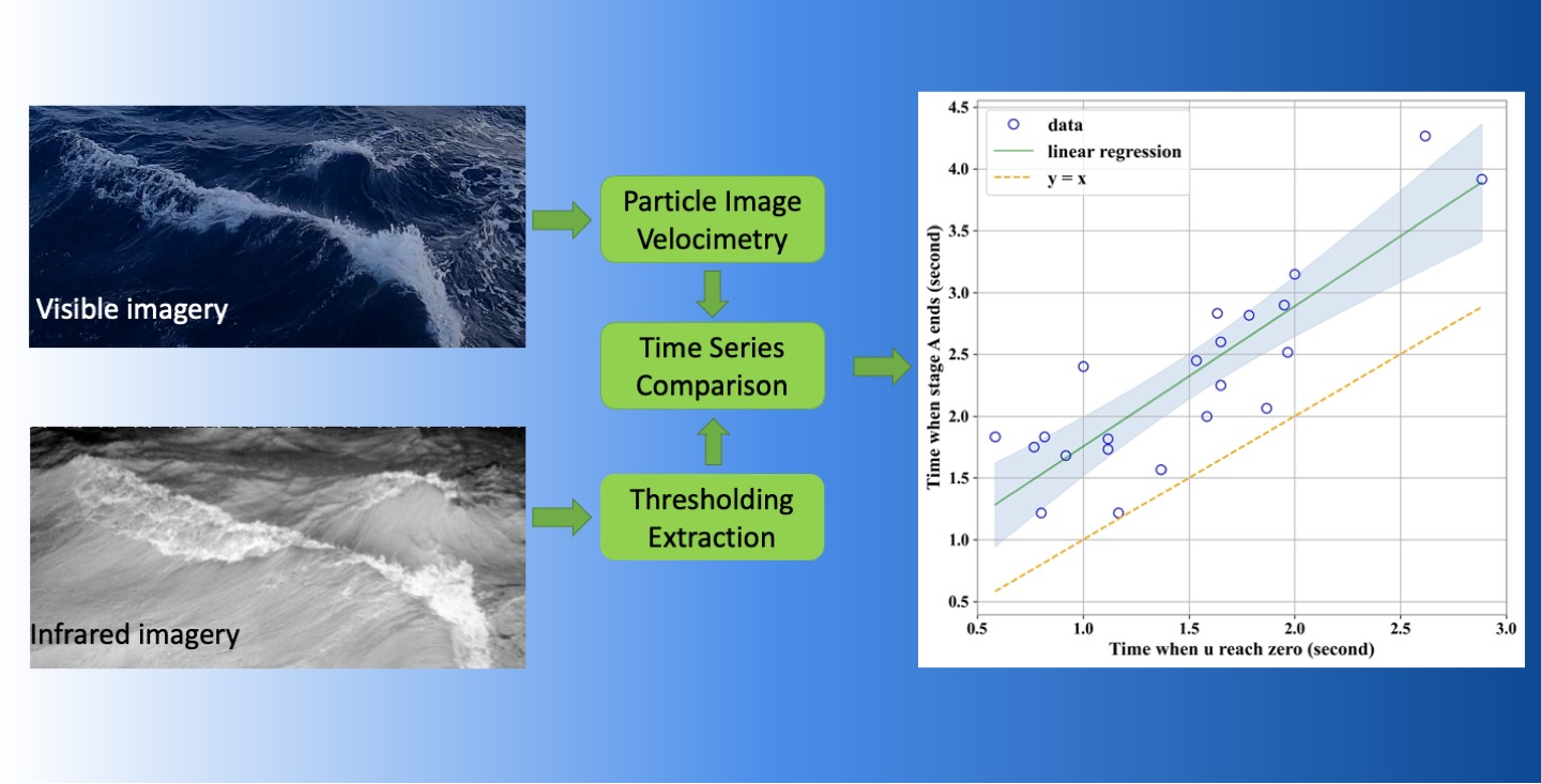
:Whitecap foam generated by wind-driven wave breaking is distinguished as either active (stage A) or residual (stage B). Discrimination of whitecap stages is essential to quantify the influence of whitecaps on the physical and chemical processes at the marine boundary layer. This study provides a novel method to identify whitecap stages based on visible imagery using particle image velocimetry (PIV). Data used are from a Gulf of Mexico cruise where collocated infrared (IR) and visible cameras simultaneously recorded whitecaps. IR images were processed by an established thresholding method to determine stage A lifetime from brightness temperature. The visible images were also filtered using a thresholding method and then processed using PIV to estimate the average whitecap velocity. A linear relationship was established between the lifetime of stage A and the timescale of averaged velocity. This novel method allows stage A whitecap lifetime to be determined using whitecap velocity and provides an objective approach to separate whitecap stages. This method paves the way for future research to easily quantify whitecap stages using affordable off-the-shelf video cameras. Results, which include evidence that whitecaps stop advancing before stage A ends and may be an indication of bubble plume degassing, are discussed.

1. Introduction
Under continued influence from the wind, waves grow until they become unstable and break. The entrainment of air during wave breaking forms bubbles in the water column which rise to the surface to form whitecaps. Whitecaps can be quantified using whitecap fraction (W), which is the percentage area of whitecaps over a region of interest. Whitecaps are often classified as either active (stage A), or residual (stage B) according to their different features during the whitecap lifetime [1]. Active whitecaps are formed and move along the crest of breaking waves. Large amounts of bubbles are generated and penetrate below the surface during stage A. The bubbles rise and provide the source for stage B, the surface foam that lingers after wave breaking. Both active and residual whitecaps contribute to whitecap fraction (i.e., W = WA + WB).
At each stage of its life, whitecaps have considerable influence on the marine boundary layer and Earth’s climate. For example, stage A marks an acoustically active period [2] with significant turbulence, energy dissipation, enhanced ocean mixing, and increased surface roughness [3]. During this stage, the entrainment of bubbles facilitates diffusion of gas into the ocean. Returning to the surface, these plumes drag water upward bringing with them surface active material, creating regions of divergence which enhance air-sea gas transfer. Stage A whitecap generation also enhances spray through the tearing of wave crests [4]. Spray droplets formed in this manner enhance sensible and latent heat fluxes and influence tropical storm intensity [4]. At stage B, the bursting of bubbles producing film and jet droplets which remain airborne often long enough to reach moisture equilibrium and transform into sea salt aerosols [5]. Sea salt aerosols have been found to increase planetary albedo directly and indirectly by acting as cloud condensation nuclei [6]. They have also been linked to the removal of atmospheric surface ozone and the activation of halogens, leading to ozone depletion [6]. Hence, the discrimination of active and residual whitecaps is essential for accurate parameterization of upper ocean processes associated with wave breaking.
Whitecap fraction has been measured extensively (e.g., [1,7,8,9,10,11,12,13,14,15,16,17]) because it is a suitable forcing variable for parameterization of a myriad of air–sea interaction processes. However, accurate parameterization requires reliable estimates of WA and WB rather than W alone because processes resulting from wave breaking may be associated with stage A or stage B, not necessarily both. A common approach is to use visible video and separate residual whitecaps from active whitecaps based on intensity thresholding [13,18]. However, despite active whitecaps generally having greater brightness than residual whitecaps [1], the continuous and subtle change of the image intensity from active to residual whitecaps makes the separation difficult. Algorithms that use image intensity or kinematic properties have made some improvement in recent years. Scanlon and Ward (2013) [17] combined intensity, texture, shape and location of whitecaps to determine the stages of whitecaps. Mironov and Dulov (2008) [19] created a set of criteria to detect whitecaps based on their propagation direction and change in area. Kleiss and Melville (2009, 2010) [20,21] also discriminated active whitecaps manually according to the criteria related to brightness and propagation direction. Despite improvements, the methods based on intensity thresholding and additional criteria remain subjective and contribute to the wide spread of WA data [22].
Satellite-based radiometric observations of the ocean surface brightness temperature TB at microwave frequencies (1–37 GHz) afford another independent method for estimating whitecap fraction W(TB) (e.g., [23]). Availability of W(TB) on a global scale over long periods provides a consistent database of W over a range of conditions. By virtue of its measuring principle, passive microwave observations of TB provide the total whitecap fraction [24]. Some work has been done to separate WA and WB from W(TB), (e.g., [16,25]), but more work is required to fully use such a database to identify stage A and stage B whitecaps independently. Efforts have also been made to model WA. For example, Kleiss and Melville (2009, 2010) [20,21] built a method based on Phillips wave breaking parameters to estimate WA. Anguelova and Hwang (2016) [22] developed a method based on Phillips theory to parameterize WA with energy dissipation rate (ε). However, both methods are parameterization models built or calibrated based on photographic data so that the subjective influence mentioned cannot be avoided [22].
Infrared (IR) imagery provides a more reliable and objective choice to discriminate active and residual whitecaps because of their different brightness at IR wavelengths. Jessup et al. (1997) [26] used infrared imaging to investigate wave breaking dissipation and temperature change due to disruption and recovery of the surface skin layer. Marmorino and Smith (2005) [27] observed both active and residual whitecaps that appear bright (warmer) and dark (cooler) respectively compared to the ambient water using airborne infrared remote sensing. Potter et al. (2015) [25] provided evidence for the dichotomic signal, i.e. signals based on two opposite criteria, from whitecaps in IR imagery and built a method to discriminate whitecaps in stage A and stage B, solely based on time series of brightness temperature. They showed that the clear dichotomic signal from whitecap foam in IR provides objective, unambiguous separation of active and residual whitecaps not readily available through other measurement techniques. This can lead to more accurate parameterization of the processes associated with each stage.
Application of IR imagery has its limitations. Principally, high resolution, fast response IR cameras necessary to capture the subtle temperature changes are orders of magnitude more expensive that off-the-shelf video cameras, often rending their use cost prohibitive. Furthermore, IR imagery systems, which are bulky yet delicate, are difficult to set up for field work especially when whitecaps are pervasive and environmental conditions can hamper operations. The maintenance of IR cameras, including the streaming system and associated hardware, also create challenges for long-term, continuous observations, meaning operating IR in remote and unmanned locations is especially challenging.
Here, a novel technique for identifying whitecap stages is introduced. This method utilizes visible and IR imagery of whitecaps captured simultaneously. Time series of thermal properties used to identify stages A and B observed in IR are compared to time series of kinematic property observed in visible imagery. It will be shown that kinematic properties of visible imagery can be used to identify whitecap stages. The technique provides a means to objectively identify whitecaps stages akin to that afforded by IR imaging while avoiding the cost and complication of IR equipment. This method of stage discrimination independent from IR imagery is invaluable for whitecaps research because it provides the opportunity to fill data gaps in WA and WB using inexpensive video cameras and some simple image processing steps. The manuscript is laid out as follows: Section 2 is the Materials and Methods, Section 3 is the Results and Discussion, and Section 4 is the Summary and Conclusions.
2. Materials and Methods
2.1. Instrumentation
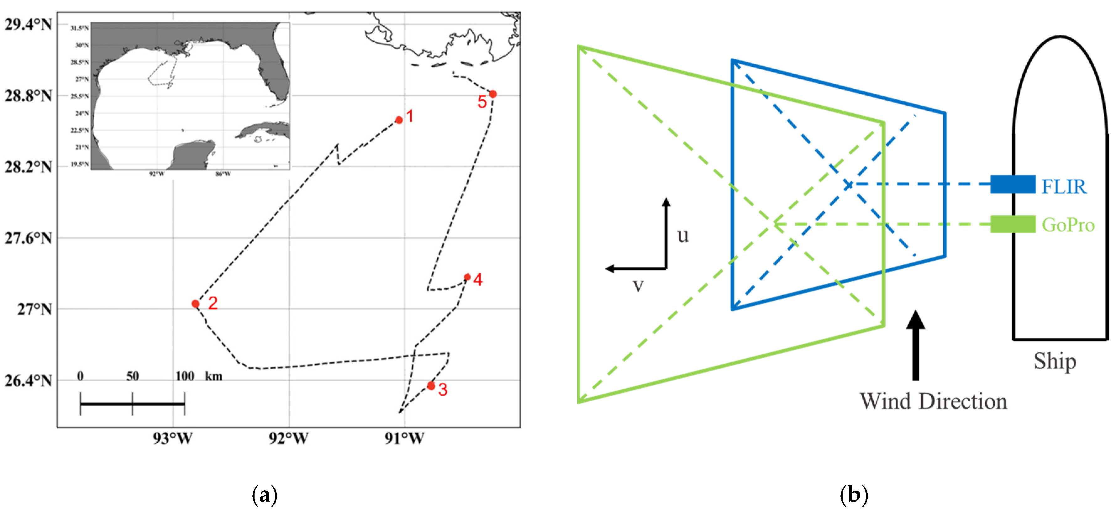
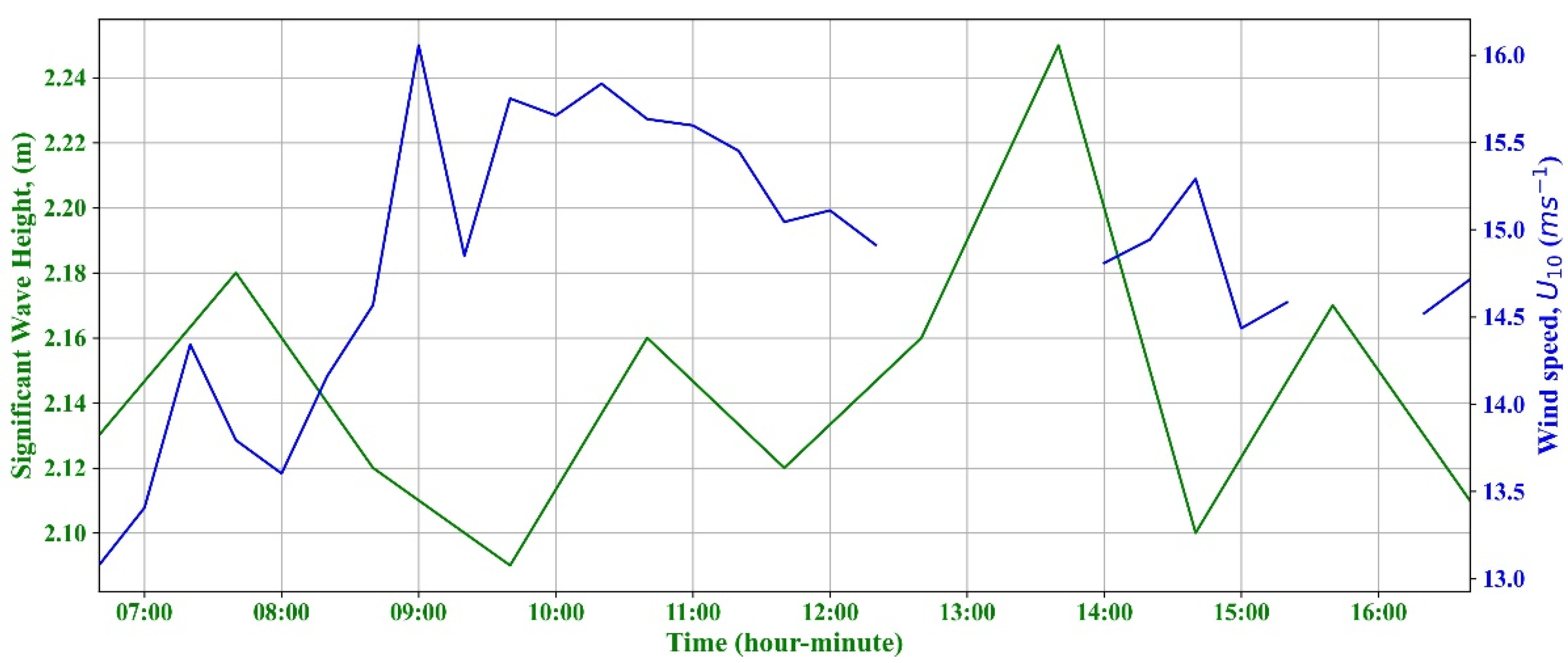
Data used here were collected during a Gulf of Mexico cruise aboard the R/V Pelican. The principal objective of this cruise was to understand whitecap foam decay using IR remote sensing. The R/V Pelican set sail on 4 March 2020 from Louisiana Universities Marine Consortium (LUMCON), Chauvin, Louisiana, and spent 5 days around 27°N, 91°W in the Gulf of Mexico. Figure 1a shows the route of the cruise. The ship stayed on the stations denoted in Figure 1a approximately 12 h each day for data collection and transited between stations at night. During the cruise, the wind speeds were in the range of 4–18 m/s and significant wave height was 1.3–2.7 m. Because of the weather condition and data quality, the events investigated in this study are all from data collected on 6 March when maximum wind speeds and significant wave height were 16 m/s and 2.2 m. Figure 2 shows the wind speed data collected onboard and significant wave height from NDBC (National Data Buoy Center) station 41040, which was the closest station with wave condition data to the ship, on 6 March. The wind speed data is at an interval of 20 min and there is data missing from 12:20 to 14:00 and from 15:20 to 16:20. The wave height data is at an interval of one hour. Two IR cameras and three visible cameras were used throughout the cruise to collect whitecap images. One of the visible cameras was mounted near the IR cameras (as is shown in Figure 1b) to make sure the footprint of IR cameras fell within that of the visible camera.
During the cruise, 50 h of video were recorded by visible cameras and over 60 h of video were recorded by infrared cameras. Three GoPro Hero 8 Black digital video cameras constituted the visible imagery system, where the linear field-of-view (FOV) lens (55.2° Vertical FOV; 85.8° Horizontal FOV; 19 mm focal length) were applied without fisheye effect. The video was recorded at 60 Hz with 1920 × 1080-pixel resolution. The infrared imagery system was comprised of a FLIR model X8500sc infrared camera (hereinafter called “FLIR camera”) and ATOM 1024 infrared camera (hereinafter called “ATOM camera”). The FLIR camera was sensitive to the radiation in the spectral range from 1.5 to 5.0 μm with a thermal sensitivity of about 0.02 K and a resolution of 1280 × 1024 pixels. The lens used in FLIR camera has 39.74° vertical FOV, 48.62° horizontal FOV and 25 mm focal length. The ATOM camera was sensitive to 8–14 μm with a thermal sensitivity of about 0.05 K and a resolution of 1024 × 768 pixels, and had a lens with 13 mm focal length, 29.27° vertical FOV and 38.39° horizontal FOV. The sampling rate of IR imagery system was 30 Hz.
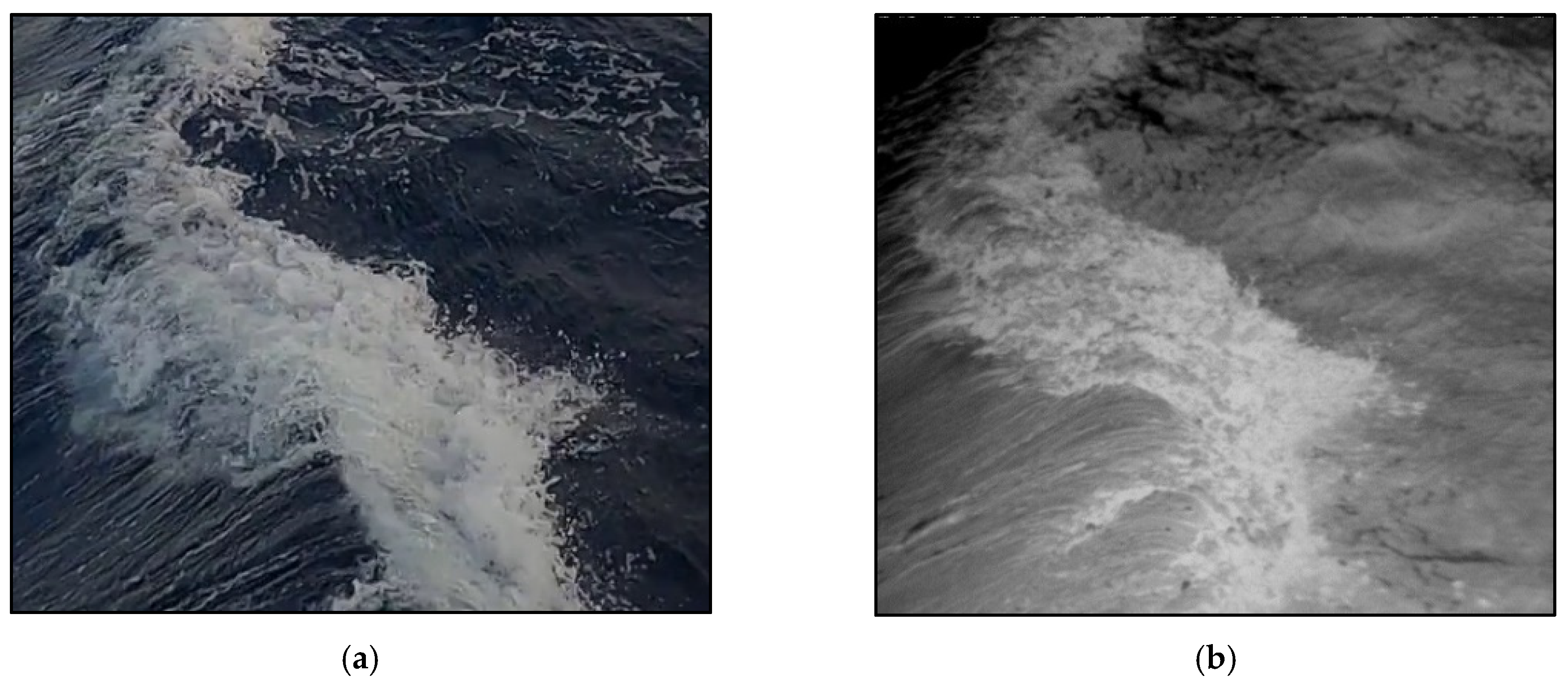
The infrared imagery system was settled in a black weather casing on the port-side at a height of 4 m above the mean water level (MWL). One of the three GoPro cameras was mounted at the top of the infrared imagery system to yield an overlapped region with the infrared cameras. The tilt angle of FLIR and ATOM cameras were both 42° (acute angle between camera axis and vertical axis at static state), while the tilt angle of GoPro camera was 74°. The tilt angle of GoPro camera was set so the horizon was visible in the images for future rectification. The FLIR camera field of view upon the water surface was ~28 m2 and the ATOM camera was ~10 m2. The overlap area between GoPro and FLIR cameras was about 16.25 m2. Figure 3a,b show the same whitecap observed simultaneously by the GoPro camera and FLIR camera. While the visible image fails to show evidence of brightness intensity difference between stages A and B, (Figure 3a), the stages are clear in IR where stage A is brighter than the ambient water and stage B is darker (Figure 3b). The two additional GoPro cameras were mounted on the port and starboard sides of the upper deck 7.6 m above the MWL. These recorded wide-angle views of the ocean surface and horizon.
2.2. Image Processing
Data from the IR system was stored in a DVR Express Core, which provided streaming of infrared images and generated RAW images with time stamps every 15 min. The GoPro camera generated MPEG-4 files every 10 min and time stamping the records by its intrinsic system.
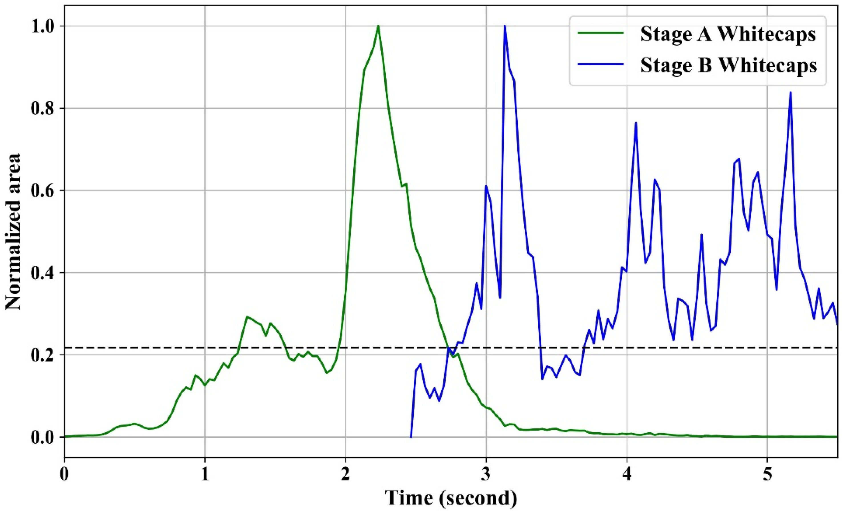
Considering dichotomic difference between whitecaps stages in IR images, thresholding is a straightforward method to separate stage A and B whitecaps from background water and the transition of whitecap lifetime stage can be identified easily. Following Potter et al. (2015) [25], for each breaking event, thresholds were applied to isolate the bright pixels (active whitecaps) and dark pixels (residual whitecaps) and used to quantify their temporal evolution. In infrared images, two threshold values are needed to identify brighter whitecaps in stage A and darker foams in stage B from ambient water. A typical outcome of this processing applied to the event is shown in Figure 4. The transition from stage A to stage B was determined to be the time when the area of stage A was less than stage B.
Particle image velocimetry (PIV) estimates the velocity field based on the correlation between image matrix segments from sequential frames [28]. It is important to remove the influence of inhomogeneous illumination on the tracers for more accurate results. During the cruise, the cameras were set at some angle to the water surface rather than orthogonally and the uneven illumination caused by the rough surface can also influence the PIV statistical analysis. In this research, the detailed fluid velocity field information is not necessary, thus some other natural tracers like wave ripples can be removed. This was done by applying a thresholding technique that has been applied previously (e.g., [28]) to isolate whitecaps for use as tracers for PIV analysis [29].
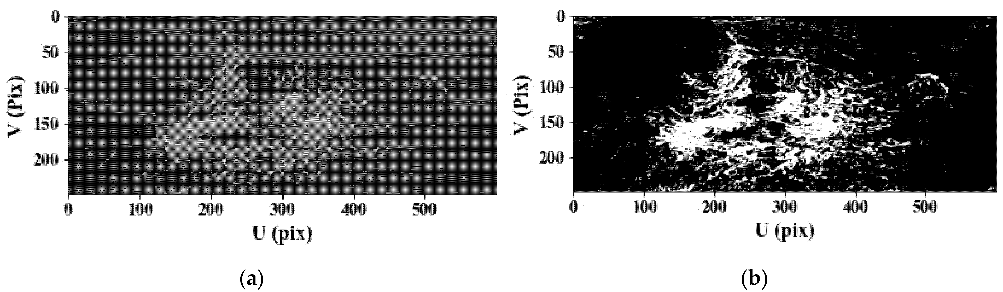
Thresholding on digital images requires determination of a suitable intensity threshold value manually or automatically to separate particles of interest from background. In visible images, whitecaps typically have a greater intensity than ambient water; hence, the whitecaps can be identified by pixels with greater intensity value than the threshold. In this research, Adaptive Thresholding Segmentation (ATS) method, created by Bakhoday-Paskyabi et al. (2016) [30], was applied to determine the threshold values for each visible and IR image. The threshold is chosen by the application of a triangle algorithm [31] to the first derivative of cumulative distribution function for pixels intensity. The algorithm was compiled and run in Python. It is a robust method with short processing time. A typical result is shown in Figure 5b.
2.3. PIV Method
PIV analyzes the correlation between small interrogation regions of subsequent frames to estimate displacement of particles to infer the velocity field [32]. PIV prevails in fluid dynamic research to determine instantaneous information about fluid velocity fields and has also been applied on larger scales to measure the surface water velocity in hydrographic studies (e.g., [33,34]). Some laboratory experiments investigating microscale breaking waves in both visible and IR imagery use PIV to estimate the kinematic properties (e.g., [35,36,37]). PIV has also been applied in oceanographic field experiments, especially when other high-resolutions measurement methods (e.g., ADCP) were absent. Melville and Matusov (2002) [29] used PIV to image sequence individual whitecaps taken from airborne cameras to estimate the normal velocity whitecap boundaries. Rüssmeier et al. (2017) [28] applied PIV to sea surface foam to estimate the surface current speed and, compared with measurement from ADCP at an offshore station, showed the reliability of PIV. Inspired by these experiments, PIV was used in this research to estimate the instantaneous velocity field during wave breaking.
Large-scale application of PIV, which is used here, applies similar algorithms to conventional PIV. However, instead of laser light and artificial tracers, which are typically used in fluid dynamic laboratory experiments (e.g., [37,38]), natural light and tracers (whitecaps) are used in this research. Therefore, the illumination can affect the PIV result significantly [33]. Enhancement of the images was recommended to improve the processing results [33]. In this research, this was done by applying a thresholding technique to extract whitecaps as tracers for PIV analysis.
Video clips that contained target whitecaps were transformed into 1920 × 1080 resolution images sequences at 60 Hz. A suitable region of interest (ROI) was chosen and cropped for each sample so that a single active whitecap was always in the frame. The whitecaps were extracted as the tracers of PIV using ATS thresholding method. PIV was realized through PIVlab, which was built in MATLAB by Thielicke and Stamhuis (2014) [39]. PIVlab provides multiple passes to do iterative calculations for better results. The interrogation area was set as 128 × 128 pixels in the first pass then 64 × 64, 32 × 32, and 16 × 16 in the following passes. Use of 2n (n is an arbitrary integer) as interrogation area is because PIVlab’s algorithm uses fast Fourier transform. The step sizes and offset between interrogation area, were set to half the width of corresponding interrogation area [39]. Examples of PIV applied to active and residual whitecaps are shown in Figure 6. The green arrows are velocity vectors calculated by PIV and result from a combination of camera motion, the velocity of breaking wave driven by wind, the surface current velocity, and the velocity of orbital motion [40]. Further discussion about the PIV results is in Section 3.1.
3. Results and Discussion
3.1. Signatures of Whitecap Lifetime Stages in PIV Results
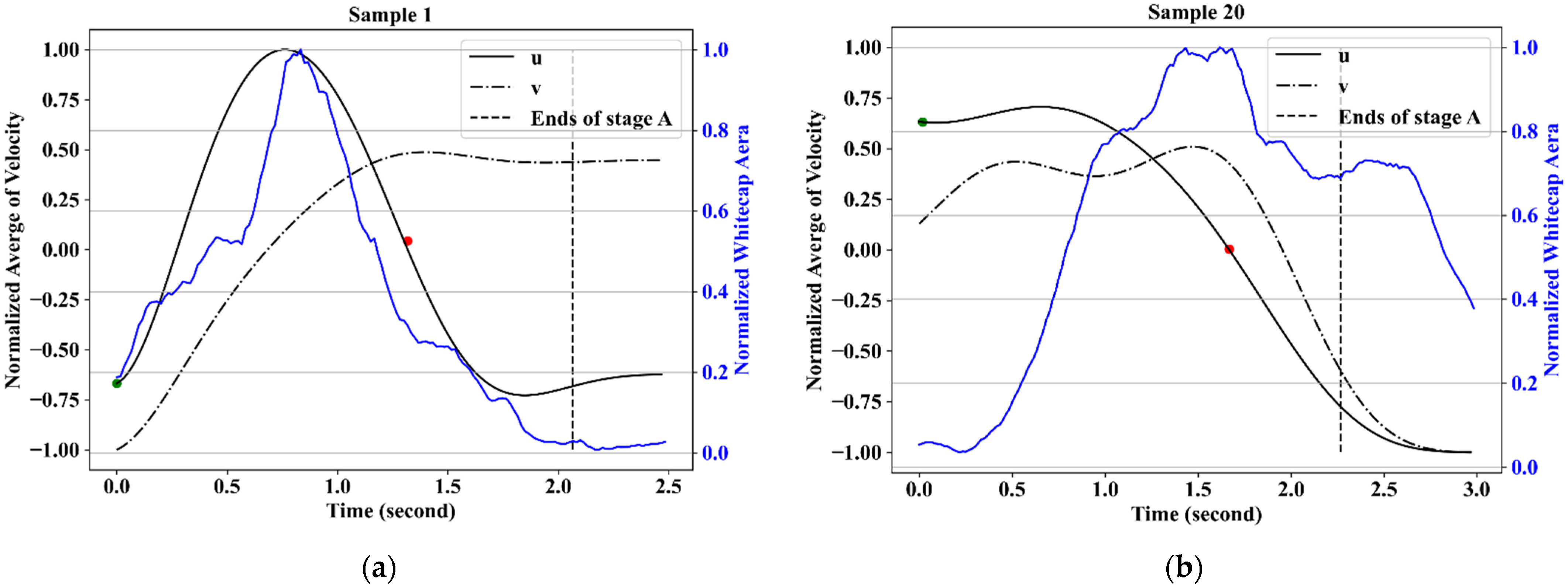
Twenty-two whitecaps were captured simultaneously by IR and visible cameras. The average velocity can be achieved from the PIV results for each frame so that a time series of the average velocity of individual whitecap can be built for an entire record of wave breaking. As mentioned, PIV results are a superposition of multiple velocities, so the average in the time domain is subtracted for each event to extract motion of whitecaps. Stage A lifetimes of all the samples are over 1 s (Table 1) and so a 1 Hz low-pass filter was applied to smooth the average velocities which could be done without losing the whitecap decay information. The velocity vectors were split into their horizontal (u) and vertical (v) components in U-V image coordinate and two types of patterns emerge, examples of which are shown in Figure 7. In the first (Figure 7a), the average horizontal and vertical velocity both show a sinusoidal-shaped curve at the beginning. In the second pattern (Figure 7b), the horizontal and vertical velocities both show an arctangent-shaped curve with the vertical velocity lagging the horizontal velocity. Ten of the twenty-two events follow the pattern in Figure 7a and twelve follow the pattern in Figure 7b.
At each station during the cruise, the ship’s bow was aligned with the wind to avoid sheltering so that more whitecaps could be observed in the ROI, and to increase ship stability which reduced inhomogeneous illumination caused by changes to the camera angle. Therefore, the direction of the wave breaking tends to be horizontal in the videos (i.e., in the u direction) as discussed in the following paragraphs.
There were two kinds of tracers, active whitecaps, and residual foam, in the images processed using PIV. The PIV result is the superposition of camera motion and the tracers’ motion. As mentioned, the tracers representing active whitecaps have three components of velocity, the velocity of breaking wave driven by wind, the surface current velocity, and the velocity of wave orbital motion [40]. The latter two components are background water velocity, and it is assumed that the temporal average is a constant. Hence, the horizontal velocity anomalies are true breaking speed under this assumption. The horizontal velocity (u) and vertical velocity (v), discussed later, are both true breaking speeds. The low-pass filter mentioned above actually removed the information about wave orbital motion, thus it will not be discussed here. The residual foam moves with the background water. In some samples, there was residual foam generated from previous wave breaking already in the ROI or flowing from nearby into the ROI. The first type of pattern (Figure 7a) describes this situation. It also accounts for why the whitecap area is not zero at the beginning of wave breaking in Figure 7a. The horizontal velocity is negative at the beginning of wave breaking and keeps increasing to positive during the growth of active whitecaps. Then the averaged horizontal velocity starts to decrease around the time when the whitecap area reaches maximum. At the end of the active stage, the averaged horizontal velocity is negative like the beginning of wave breaking. In the second type of pattern (Figure 7b), there is no preexisting residual foam. The averaged horizontal velocity, u, appears to continue to decrease in magnitude until it reaches zero, and then increases in magnitude in the reverse direction, as the active whitecaps approach the line designating the residual whitecap regime. Therefore, the existence of tracers of background water at the beginning of wave breaking likely account for the different temporal velocity patterns.
3.2. Linear Regression Model
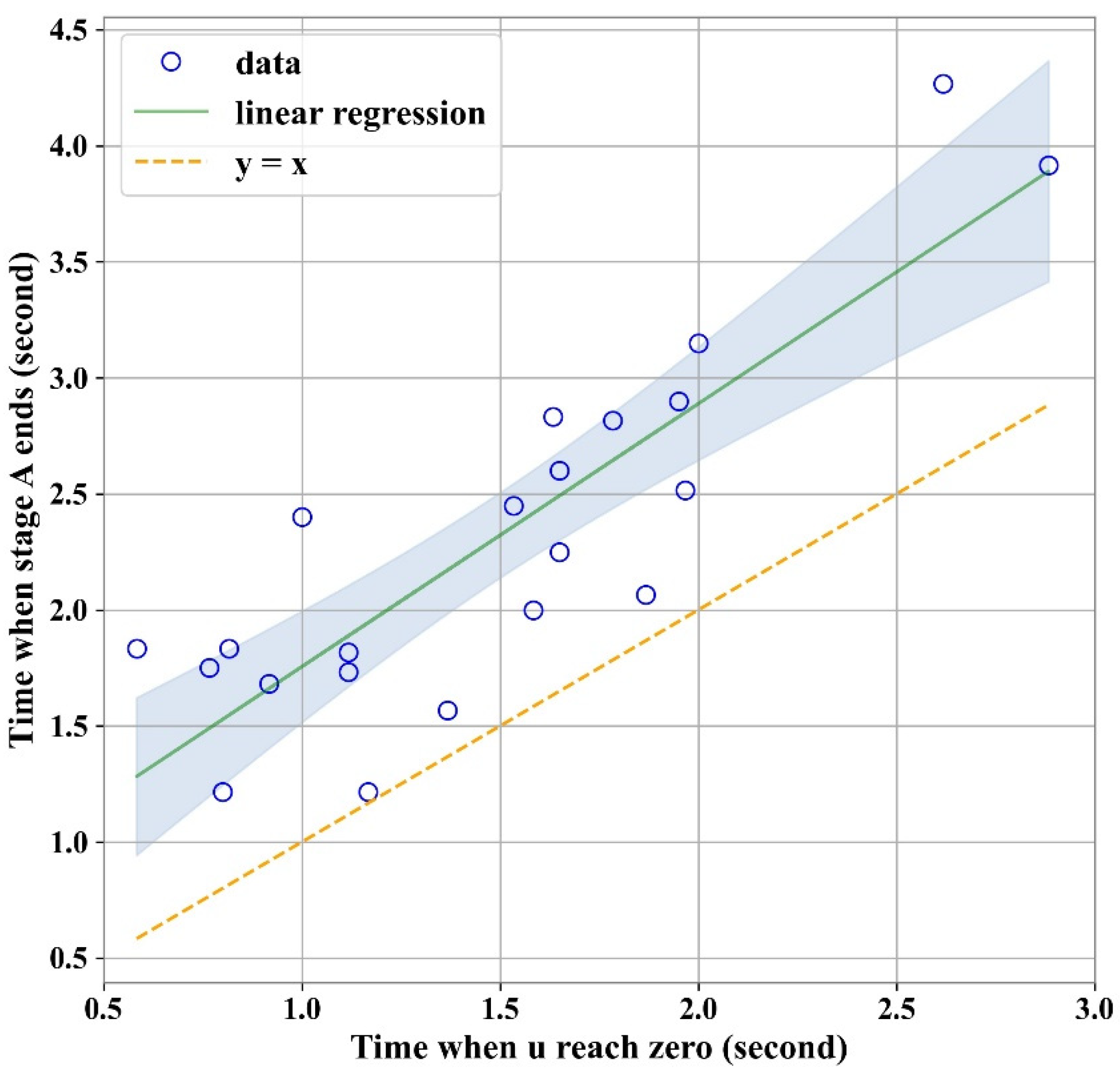
Whitecaps are formed by wave breaking under the influence of wind. Therefore, to a greater or lesser extent, the parameters related to wind and surface water state can influence whitecaps. Tracking individual whitecaps, the waves grow and break as they move forward. Active whitecaps outpace the ambient water, while residual foam flows with the surface water. This phenomenon suggests that velocity variation of an individual breaking wave is related to the lifetime stages of whitecaps. Jessup et al. (1997) [26] found a linear relationship between the centroid speed of active whitecaps and the recovery time of the skin layer after wave breaking, which can be used to estimate stage A whitecaps lifetime. In this study, with the advantage of whitecaps recorded simultaneously using IR and visible remote sensing, the relationship between time scales of kinematic variation and thermal variation can be determined. The time when a stage A whitecap ends, as quantified using IR, is compared with the time when the averaged horizontal velocity finally reaches zero after the peak. The results for all 22 waves are shown in Figure 8. Coefficient of determination, r2, is 0.738, and the linear model is:
where TA is the time taken for stage A of a whitecap to end, and TV is the time when the averaged horizontal velocity of a whitecap finally reaches zero relative to the beginning of wave breaking. Table 2 shows the results of statistical testing and linear regression coefficients. The linear relationship can be interpreted that the lifetime of an active whitecap is proportional to the timescale of breaking speed. Therefore, TA and TV in Equation (1) can be replaced with the lifetime of stage A and the time it takes for a whitecap’s speed to reach zero, respectively. With the help of this linear model, one can apply PIV to visible imagery and substitute the time scale of the breaking speed to estimate the lifetime of stage A. With this information, it can be determined whether a whitecap is in stage A or stage B.
TA = 1.134 × TV + 0.621
Discrimination of whitecaps stages in this method only requires visible videos. The quality of the images is important for the implementation. Uneven illumination and sun glint are two main factors that can contaminate images [9]. Uneven illumination usually happens when the sea surface is rough, especially around the beginning of wave breaking. Some areas of ambient water can have similar intensity to whitecaps due to uneven illumination which may lead to the failure of whitecaps extraction through thresholding. The changing illumination makes the bright areas appear to move faster than the real surface water velocity in the PIV algorithm. The situation can be worse at the beginning of stage A because the number of the real tracers is small so uneven illumination can have a bigger influence on the average velocity. Uneven illumination can also affect the pixels filtered by thresholding. Overestimation of active or residual foam through image processing can lead to errors in the average. The sun glint affects the prediction result in the similar way to uneven illumination. Normally, the image sequence contaminated by sun glint should be discarded, while the influence of uneven illumination can be avoided by omitting the contaminated images at the beginning of wave breaking or increase the threshold value to filter the contaminated area. Increasing the threshold value can filter some pixels representing whitecaps, but it will not affect the estimate of PIV since the quantification of whitecap fraction is not the purpose of this method.
According to the linear regression result (Figure 8), the average velocity of whitecaps reaches zero earlier than whitecap stage A ends. Two factors may lead to this situation. First, the average velocity reaches zero before the breaking ends. The breaking front proceeds forward while foam after the crest moves in the opposite direction resulting in zero average velocity before stage A ends. Second, the breaking waves stop moving but keep degassing, especially when the penetration depth of bubbles is deep. Callaghan et al. (2013, 2016) [41,42] conducted a laboratory experiment to explore whitecap foam decay, where breaking waves were generated in a seawater channel and recorded with above and side-mounted cameras. They found that whitecap lifetime was a function of wave scale, with larger waves having longer whitecap lifetime [41]. A positive power law relationship between whitecap lifetime and averaged bubble penetration depth was also built in their study [42]. However, there appears to be no direct evident that establishes a relationship between penetration depth and stage A lifetime. It is possible that the penetration depth affects stage B lifetime therefore the whitecap lifetime as a whole. Callaghan et al. (2016) [42] built a model to predict breaking dissipation based on volume time-integral, which is the product of whitecap area, averaged penetration depth and growth timescale (timescale of the whitecap area increase). The breaking dissipation has a positive linear relationship with the volume time-integral [42]. Jessup et al. (1997) [26] found a positive linear relationship between stage A lifetime and velocity of breaking front. Under the assumption that the velocity of breaking front is related to the breaking dissipation, it can be inferred that the volume time-integral has a positive relationship with stage A lifetime based on the research mentioned above. It is indicated that the wave scale and the penetration depth have a positive influence on stage A lifetime. To explore this, we conducted a simple experiment using an off-the-shelf bubble maker typically used in aquariums and a small tank. FLIR was used to observe the bubbles on the water surface. The foam temperature showed no observable decrease until the foam remained on the surface for some time after the bubble generator had been turned off. Masnadi et al. (2020) [43] found that cooling of surface foam is delayed until the rate of renewal of the foam by rising bubbles is less than the foam cooling rate. The same mechanism is likely responsible for the delayed cooling observed in the lab and supports the theory that whitecaps observed in IR remain in stage A briefly after breaking velocity reaches zero due to bubble plume dynamics. Masnadi et al. (2020) performed excellent work quantifying the relationship between whitecap temperature and bubble plume decay in the lab but more information about the factors affecting the cooling time-delay, especially at sea, are needed to fully understand why velocity reaches zero before stage A ends.
During wave breaking, wave energy is dissipated through turbulence. The entraining air rises and forms bubbles on the surface, which enlarge the contact area between air and water aiding temperature loss [27]. Stage B whitecaps are a manifestation of this process [25,27]. However, it remains uncertain whether stage B whitecaps identified using IR start during the rising of bubbles or sometime after the bubbles reach the surface. The dissipation process of wave breaking can therefore be divided into two phases, kinetic dissipation dominated by turbulence and internal dissipation dominated by evaporative cooling. It is possible that the kinetic dissipation happens before the internal dissipation so that the breaking crest stops moving before degassing. It is worth further research to clarify the energy transfer during wave breaking.
4. Summary and Conclusions
Under continued influence from the wind, waves grow until they become unstable and break creating whitecaps. These whitecaps are distinguished as either actively generated (stage A) or decaying (stage B). Stage A whitecaps are formed along the crest of a wave during breaking, stage B are the patches left on the surface. Whitecap coverage is quantified by whitecap fraction W (W = WA + WB). At each stage of its life, whitecaps have considerable influence on the marine boundary layer so discrimination of whitecaps stages is critical to accurately quantify momentum and mass transfer. Whitecap stages are easily identified in IR by their dichotomic characteristics but subtle change of image intensity from active to residual stages makes the separation difficult at visible wavelengths. This study provides a novel method to distinguish whitecap stages by applying PIV to visible imagery. This highly accessible and practical method paves the way for affordable, user-friendly cameras to advance whitecap research through improved quantification and understanding of WA and WB.
Data were collected during a Gulf of Mexico cruise where breaking waves were captured simultaneously using collocated IR and visible video cameras. The visible images were processed using ATS thresholding to extract whitecaps from background features and PIV to determine the average tracer (whitecaps) velocity. IR images were also processed with ATS thresholding technique to distinguish stage A whitecaps from the ambient background. Averaged velocity was then compared to the lifetime of stage A. Twenty-two samples were processed this way. A linear relationship was established between the lifetime of stage A and the timescale of averaged velocity. Hence, substitution of the timescale of averaged velocity into the linear model presented yields the stage A whitecap lifetime.
The linear regression indicates that the velocity of whitecap reaches zero before whitecap stage A ends, with an average delay of ~1 s. Two possible reasons for this are discussed. The first is the potential non-uniform breaking velocity across an individual whitecap that results in zero average before the breaking front stops advancing. The second is that whitecap cooling is delayed due to the inequity in rates of foam cooling and renewal as identified by Masnadi et al. (2020) [43]. This would have implication for breaking wave mechanics such as bubble penetration depth and degassing time. Some evidence is provided to support the second hypothesis, but further investigation is needed.
Author Contributions
Conceptualization, H.P.; Methodology, Yang; Software, Yang; Validation, Yang; Formal Analysis, X.Y.; Investigation, H.P. and X.Y.; Resources, H.P.; Data Curation, X.Y.; Writing—Original Draft Preparation, H.P. and X.Y.; Writing—Review and Editing, H.P.; Visualization, X.Y.; Supervision, H.P.; Project Administration, H.P.; Funding Acquisition, H.P. All authors have read and agreed to the published version of the manuscript.
Funding
This research was funded by the National Science Foundation under grant 1829986. Additional funding was provided by Texas A&M department of oceanography to help support the dozen graduate and undergraduate students who participated in the research cruises.
Data Availability Statement
Cruise data are available through the Rolling Deck to Repository (R2R) https://www.rvdata.us (accessed on 6 October 2021) for cruises PE20-08 and PE20-17. Whitecap lifetime extracted from visible and infrared video is archived at National Ocean Data Center. Raw video footage is available upon request by contacting the corresponding author.
Acknowledgments
We are very grateful to Geoff Smith of the Naval Research Laboratory Remote Sensing Division who provided equipment and operational support during both cruises as well as post-processing expertise. We thank the captain and crew of the R/V Pelican for two successful cruises. Finally, we express our appreciation to the dozen graduate and undergraduate students who all contributed to success of the research cruises.
Conflicts of Interest
The authors declare no conflict of interest.
References
- Monahan, E.C.; Woolf, D.K. Comments on “Variations of whitecap coverage with wind stress and water temperature”. J. Phys. Oceanogr. 1989, 19, 706–709. [Google Scholar] [CrossRef] [Green Version]
- Monahan, E.C.; Lu, M. Acoustically Relevant Bubble Assemblages and Their Dependence on Meteorological Parameters. IEEE J. Ocean. Eng. 1990, 15, 340–349. [Google Scholar] [CrossRef]
- Padmanabhan, S.; Rose, L.A.; Gaiser, P.W. Effects of foam on ocean surface microwave emission inferred from radiometric observations of reproducible breaking waves. IEEE Trans. Geosci. Remote Sens. 2006, 44, 569–582. [Google Scholar] [CrossRef]
- Andreas, E.L.; Emanuel, K.A. Effects of sea spray on tropical cyclone intensity. J. Atmos. Sci. 2001, 58, 3741–3751. [Google Scholar] [CrossRef] [Green Version]
- Blanchard, D.C. The production, distribution, and bacterial enrichment of the sea-salt aerosol. In Air-Sea Exchange of Gases and Particles; Springer: Dordrecht, The Netherlands, 1983; pp. 407–454. [Google Scholar]
- Lewis, E.R.; Lewis, R.; Lewis, E.R.; Schwartz, S.E. Sea Salt Aerosol Production: Mechanisms, Methods, Measurements, and Models; American Geophysical Union: Washington, DC, USA, 2004; Volume 152, ISBN 0875904173. [Google Scholar]
- Monahan, E.C. Oceanic whitecaps. J. Phys. Oceanogr. 1971, 1, 139–144. [Google Scholar] [CrossRef]
- Brumer, S.E.; Zappa, C.J.; Brooks, I.M.; Tamura, H.; Brown, S.M.; Blomquist, B.W.; Fairall, C.W.; Cifuentes-Lorenzen, A. Whitecap coverage dependence on wind and wave statistics as observed during SO GasEx and HiWinGS. J. Phys. Oceanogr. 2017, 47, 2211–2235. [Google Scholar] [CrossRef]
- Callaghan, A.H.; White, M. Automated processing of sea surface images for the determination of whitecap coverage. J. Atmos. Ocean. Technol. 2009, 26, 383–394. [Google Scholar] [CrossRef]
- Monahan, E.C.; O’Muircheartaigh, I.G. Whitecaps and the passive remote sensing of the ocean surface. Int. J. Remote Sens. 1986, 7, 627–642. [Google Scholar] [CrossRef]
- Wu, J. Variations of whitecap coverage with wind stress and water temperature. J. Phys. Oceanogr. 1988, 18, 1448–1453. [Google Scholar] [CrossRef] [Green Version]
- Xu, D.; Liu, X.; Yu, D. Probability of wave breaking and whitecap coverage in a fetch-limited sea. J. Geophys. Res. Oceans 2000, 105, 14253–14259. [Google Scholar] [CrossRef]
- Asher, W.; Edson, J.; McGillis, W.; Wanninkhof, R.; Ho, D.T.; Litchendorf, T. Fractional area whitecap coverage and air-sea gas transfer velocities measured during GasEx-98. Geophys. Monogr. Ser. 2001, 127, 199–203. [Google Scholar] [CrossRef]
- Anguelova, M.D.; Webster, F. Whitecap coverage from satellite measurements: A first step toward modeling the variability of oceanic whitecaps. J. Geophys. Res. Oceans 2006, 111. [Google Scholar] [CrossRef] [Green Version]
- Lafon, C.; Piazzola, J.; Forget, P.; Despiau, S. Whitecap coverage in coastal environment for steady and unsteady wave field conditions. J. Mar. Syst. 2007, 66, 38–46. [Google Scholar] [CrossRef]
- Salisbury, D.J.; Anguelova, M.D.; Brooks, I.M. On the variability of whitecap fraction using satellite-based observations. J. Geophys. Res. Oceans 2013, 118, 6201–6222. [Google Scholar] [CrossRef] [Green Version]
- Scanlon, B.; Ward, B. Oceanic wave breaking coverage separation techniques for active and maturing whitecaps. Methods Oceanogr. 2013, 8, 1–12. [Google Scholar] [CrossRef]
- Hanson, J.L.; Phillips, O.M. Wind sea growth and dissipation in the open ocean. J. Phys. Oceanogr. 1999, 29, 1633–1648. [Google Scholar] [CrossRef]
- Mironov, A.S.; Dulov, V.A. Detection of wave breaking using sea surface video records. Meas. Sci. Technol. 2008, 19, 015405. [Google Scholar] [CrossRef]
- Kleiss, J.M. Airborne Observations of the Kinematics and Statistics of Breaking Waves. Ph.D. Thesis, UC San Diego, San Diego, CA, USA, 2009. [Google Scholar]
- Kleiss, J.M.; Melville, W.K. Observations of wave breaking kinematics in fetch-limited seas. J. Phys. Oceanogr. 2010, 40, 2575–2604. [Google Scholar] [CrossRef]
- Anguelova, M.D.; Hwang, P.A. Using energy dissipation rate to obtain active whitecap fraction. J. Phys. Oceanogr. 2016, 46, 461–481. [Google Scholar] [CrossRef]
- Anguelova, M.D.; Gaiser, P.W.; Raizer, V. Foam emissivity models for microwave observations of oceans from space. Int. Geosci. Remote Sens. Symp. 2009, 2, 274–277. [Google Scholar] [CrossRef]
- Anguelova, M.D.; Gaiser, P.W. Skin depth at microwave frequencies of sea foam layers with vertical profile of void fraction. J. Geophys. Res. Oceans 2011, 116, 1–15. [Google Scholar] [CrossRef] [Green Version]
- Potter, H.; Smith, G.B.; Snow, C.M.; Dowgiallo, D.J.; Bobak, J.P.; Anguelova, M.D. Whitecap lifetime stages from infrared imagery with implications for microwave radiometric measurements of whitecap fraction. J. Geophys. Res. Oceans 2015, 120, 7521–7537. [Google Scholar] [CrossRef]
- Jessup, A.T.; Zappa, C.J.; Loewen, M.R.; Hesany, V. Infrared remote sensing of breaking waves. Nature 1997, 385, 52–55. [Google Scholar] [CrossRef]
- Marmorino, G.O.; Smith, G.B. Bright and dark ocean whitecaps observed in the infrared. Geophys. Res. Lett. 2005, 32, 1–4. [Google Scholar] [CrossRef]
- Russmeier, N.; Hahn, A.; Zielinski, O. Ocean surface water currents by large-scale particle image velocimetry technique. In Proceedings of the OCEANS 2017—Aberdeen, Aberdeen, UK, 19–22 June 2017; pp. 1–10. [Google Scholar] [CrossRef]
- Melville, W.K.; Matusov, P. Distribution of breaking waves at the ocean surface. Nature 2002, 417, 58–63. [Google Scholar] [CrossRef]
- Bakhoday-Paskyabi, M.; Reuder, J.; Flügge, M. Automated measurements of whitecaps on the ocean surface from a buoy-mounted camera. Methods Oceanogr. 2016, 17, 14–31. [Google Scholar] [CrossRef]
- Zack, G.W.; Rogers, W.E.; Latt, S.A. Automatic measurement of sister chromatid exchange frequency. J. Histochem. Cytochem. 1977, 25, 741–753. [Google Scholar] [CrossRef] [PubMed]
- Westerweel, J. Fundamentals of digital particle image velocimetry. Meas. Sci. Technol. 1997, 8, 1379–1392. [Google Scholar] [CrossRef] [Green Version]
- Fujita, I.; Muste, M.; Kruger, A. Large-scale particle image velocimetry for flow analysis in hydraulic engineering applications. J. Hydraul. Res. 1998, 36, 397–414. [Google Scholar] [CrossRef]
- Legleiter, C.J.; Kinzel, P.J.; Nelson, J.M. Remote measurement of river discharge using thermal particle image velocimetry (PIV) and various sources of bathymetric information. J. Hydrol. 2017, 554, 490–506. [Google Scholar] [CrossRef]
- Jessup, A.T.; Phadnis, K.R. Measurement of the geometric and kinematic properties of microscale breaking waves from infrared imagery using a PIV algorithm. Meas. Sci. Technol. 2005, 16, 1961–1969. [Google Scholar] [CrossRef]
- Techet, A.H.; McDonald, A.K. High Speed PIV of Breaking Waves on Both Sides of the Air-Water Interface. In Proceedings of the 6th International Symposium on Particle Image Velocimetry, Pasadena, CA, USA, 21–23 September 2005; pp. 1–14. [Google Scholar]
- Siddiqui, M.H.K.; Loewen, M.R.; Richardson, C.; Asher, W.E.; Jessup, A.T. Simultaneous particle image velocimetry and infrared imagery of microscale breaking waves. Phys. Fluids 2001, 13, 1891–1903. [Google Scholar] [CrossRef]
- Grant, I. Particle image velocimetry: A review. Proc. Inst. Mech. Eng. Part C J. Mech. Eng. Sci. 1997, 211, 55–76. [Google Scholar] [CrossRef]
- Thielicke, W.; Stamhuis, E.J. PIVlab-time-resolved digital particle image velocimetry tool for MATLAB. Publ. BSD Licens. Program. MATLAB 2014, 7, R14. [Google Scholar]
- Callaghan, A.H.; Deane, G.B.; Stokes, M.D.; Ward, B. Observed variation in the decay time of oceanic whitecap foam. J. Geophys. Res. Oceans 2012, 117. [Google Scholar] [CrossRef] [Green Version]
- Callaghan, A.H.; Deane, G.B.; Stokes, M.D. Two regimes of laboratory whitecap foam decay: Bubble-plume controlled and surfactant stabilized. J. Phys. Oceanogr. 2013, 43, 1114–1126. [Google Scholar] [CrossRef]
- Callaghan, A.H.; Deane, G.B.; Stokes, M.D. Laboratory air-entraining breaking waves: Imaging visible foam signatures to estimate energy dissipation. Geophys. Res. Lett. 2016, 43, 11320–11328. [Google Scholar] [CrossRef]
- Masnadi, N.; Chickadel, C.C.; Jessup, A.T. On the Thermal Signature of the Residual Foam in Breaking Waves. J. Geophys. Res. Oceans 2021, 126, e2020JC016511. [Google Scholar] [CrossRef]
Figure 1.
(a) Route of the cruise (red dots denote the stations); (b) schematic of cameras fields of view: the FLIR (blue) is an IR camera, the GoPro (green) is a visible camera.
Figure 1.
(a) Route of the cruise (red dots denote the stations); (b) schematic of cameras fields of view: the FLIR (blue) is an IR camera, the GoPro (green) is a visible camera.

Figure 2.
Wind speed and significant wave height conditions for 6 March when the IR and visible imagery analyzed in this study were collected.
Figure 2.
Wind speed and significant wave height conditions for 6 March when the IR and visible imagery analyzed in this study were collected.

Figure 3.
(a) Whitecaps include active and residual foams in a visible image; (b) whitecaps include active and residual foams in an IR image. The bright patches are active whitecaps, and the dark patches are residual whitecaps.
Figure 3.
(a) Whitecaps include active and residual foams in a visible image; (b) whitecaps include active and residual foams in an IR image. The bright patches are active whitecaps, and the dark patches are residual whitecaps.

Figure 4.
Time series of infrared signal of a breaking event. Stage A whitecaps are determined by bright area, and stage B whitecaps are determined by dark areas. The whitecaps areas are normalized by their respective maximums. The dashed line denotes the normalized area when the area of stage A was less than stage B.

Figure 5.
(a) Residual whitecaps in a visible image; (b) thresholding result of the left panel.

Figure 6.
(a) An active whitecap in a visible image; (b) PIV result of the whitecap in the left panel; (c) a residual whitecap in a visible image; (d) PIV result of the whitecap in the left panel.
Figure 6.
(a) An active whitecap in a visible image; (b) PIV result of the whitecap in the left panel; (c) a residual whitecap in a visible image; (d) PIV result of the whitecap in the left panel.

Figure 7.
Time series of average u and v velocity of whitecap foam and normalized whitecap area. (a,b) are examples of the two types of velocity patterns as discussed in the text. The green dots denote the beginning of wave breaking according to IR images. The red dots denote the last time when the horizontal velocity changes direction. The vertical dash lines denote the end of stage A.

Figure 8.
Time when stage A ends against time when averaged horizontal velocity finally reaches zero (changes direction) in the same image sequence. The green line is the least squares linear regression and the shaded area is the 95% confidence interval. The orange-dashed line, y = x, is plotted for comparison.


Table 1.
Lifetime of active whitecaps in this study.
| Lifetime of Active Whitecaps (s) | Number |
|---|---|
| 1–2 | 10 |
| 2–3 | 9 |
| >3 | 3 |
Table 2.
Linear regression summary for predicting stage A end time.
| Coefficient | 95% CI 1 | t | p | |
|---|---|---|---|---|
| Intercept | 0.621 | [0.118 1.125] | 2.575 | 0.018 |
| slope | 1.134 | [0.819 1.448] | 7.515 | 0.000 |
1 CI = confidence interval.
Publisher’s Note: MDPI stays neutral with regard to jurisdictional claims in published maps and institutional affiliations. |
© 2021 by the authors. Licensee MDPI, Basel, Switzerland. This article is an open access article distributed under the terms and conditions of the Creative Commons Attribution (CC BY) license (https://creativecommons.org/licenses/by/4.0/).
Share and Cite
MDPI and ACS Style
Yang, X.; Potter, H. A Novel Method to Discriminate Active from Residual Whitecaps Using Particle Image Velocimetry. Remote Sens. 2021, 13, 4051. https://doi.org/10.3390/rs13204051
AMA Style
Yang X, Potter H. A Novel Method to Discriminate Active from Residual Whitecaps Using Particle Image Velocimetry. Remote Sensing. 2021; 13(20):4051. https://doi.org/10.3390/rs13204051
Chicago/Turabian StyleYang, Xin, and Henry Potter. 2021. "A Novel Method to Discriminate Active from Residual Whitecaps Using Particle Image Velocimetry" Remote Sensing 13, no. 20: 4051. https://doi.org/10.3390/rs13204051
Note that from the first issue of 2016, this journal uses article numbers instead of page numbers. See further details here.