Narrowband and Wideband Channel Sounding of an Antarctica to Spain Ionospheric Radio Link

Abstract

La Salle and Ebro Observatory have been involved in remote sensing projects in Antarctica for the last 11 years (approximately one solar cycle). The Ebro Observatory has been monitoring and analyzing the geomagnetic and the ionospheric activity in the Antarctic Spanish station Juan Carlos I (ASJI) (62.7°S, 299.6°E) for more than eighteen and ten years, respectively. La Salle has two main goals in the project. The first one is the data transmission and reception from Antarctica to Spain to obtain a historical series of measurements of channel sounding of this 12,760-km ionospheric HF (high frequency) radio link. The second one is the establishment of a stable data low power communication system between the ASJI and Cambrils, Spain (41.0°N, 1.0°E), to transmit the data from the remote sensors located on the island. In this paper, both narrowband and wideband soundings have been carried out to figure out the channel availability performed using a frequency range from 2 to 30 MHz with 0.5 MHz step during the 24 h of the day, encompassing wider channel measurements than previously done, in terms of hours and frequency. This paper presents the results obtained for the austral summer in 2014, using a monopole antenna at the transmitter and an inverted V on the receiver side. These results led us to the final physical layer design for the long haul link, dividing the day into two parts: daytime, with low data throughput design, and nighttime, reaching high data throughput.

1. Introduction

Analyzing the ionosphere and the magnetic field in Antarctica is an important contribution to understand the Earth’s phenomena concerning geophysical science. Knowledge acquired on the characteristics of the channel does not only improve the performance of high frequency (HF) radio-communication systems, but also contributes to ionospheric science, for example ionospheric noises are found to affect the HF radar-based ocean current mapping [1,2]. Vertical and oblique sounding techniques are frequently used to obtain the characteristics of the ionospheric communications channel for a given radio link. The geomagnetic observatories have been the magnetic field variations in fixed locations collecting for years, having a wide range of time scales, from seconds to centuries, to make the understanding of the behavior of the magnetic field of the Earth possible.

The Antarctic Spanish station Juan Carlos I (ASJI) is located on Livingston Island, a place of great interest, because it monitors the sub-auroral zone [3]. The ASJI has a geomagnetic observatory with the International Association of Geomagnetism and Aeronomy Code LIV. LIV is remotely managed by the Ebro Observatory Institute (EO) in Spain, and it is aimed at monitoring the magnetic field variations of that region. ASJI is only attended by scientist and technicians during the austral summer, typically from December to February. As ionospheric exploration by vertical soundings is one of the most commonly-used methods to observe the vertical structure of the ionosphere, a VIS (vertical incidence sounder) was installed at the ASJI during the summer expedition of 2004 to 2005 by OE. In 2003, an OIS (oblique incidence sounder) was also installed at the ASJI by La Salle with a double objective: (i) to measure the characteristics of the ionospheric channel from ASJI to Spain, taking into account days, annual and solar cycle variations; and (ii) to install a robust hardware and software platform for an HF radio-communication system from ASJI to Spain. The latter system should be able to operate under hard environmental conditions, with the best digital modulations designed for a low power and high interference communications system. The OIS covers a long haul ionospheric link (see Figure 1), of around 12,760 km, from the ASJI (62.7°S, 299.6°E) to Cambrils (41.0°N, 1.0°E).

In previous works, both narrowband and wideband soundings had been analyzed [4], but both carrier frequencies and the time of transmission were limited. Since 2008, an enhanced transmitter and receiver were installed [5], and the oblique sounding observations can be widely recorded. The results presented in this paper shed light on the knowledge of this long haul link, but also help us to design the physical layer characteristics remaining from previous studies [6,7,8], where less carrier frequencies were used and the tests were not performed during the entire day.

This paper is organized as follows. Section 2 describes all of the measured parameters. Section 3 gives the details of the communications hardware equipment between the Remote Geophysical Observatory and Spain. Section 4 explains the test design for narrowband and wideband sounding measurements through a long-distance HF link in the 2014 campaign. Section 5 presents the results of the sounding measurements. Finally, Section 6 contains the conclusions and the future work.

Figure 1. Geographical link characteristics. The transmitter is located at the Antarctic Spanish station Juan Carlos I (ASJI), on Livingston Island (62.7°S, 299.6°E), and the receiver is placed in Cambrils (41.0°N, 1.0°E).

Figure 1. Geographical link characteristics. The transmitter is located at the Antarctic Spanish station Juan Carlos I (ASJI), on Livingston Island (62.7°S, 299.6°E), and the receiver is placed in Cambrils (41.0°N, 1.0°E).

2. Measured Parameters

This section describes the main sensors located at the ASJI and its measurements.

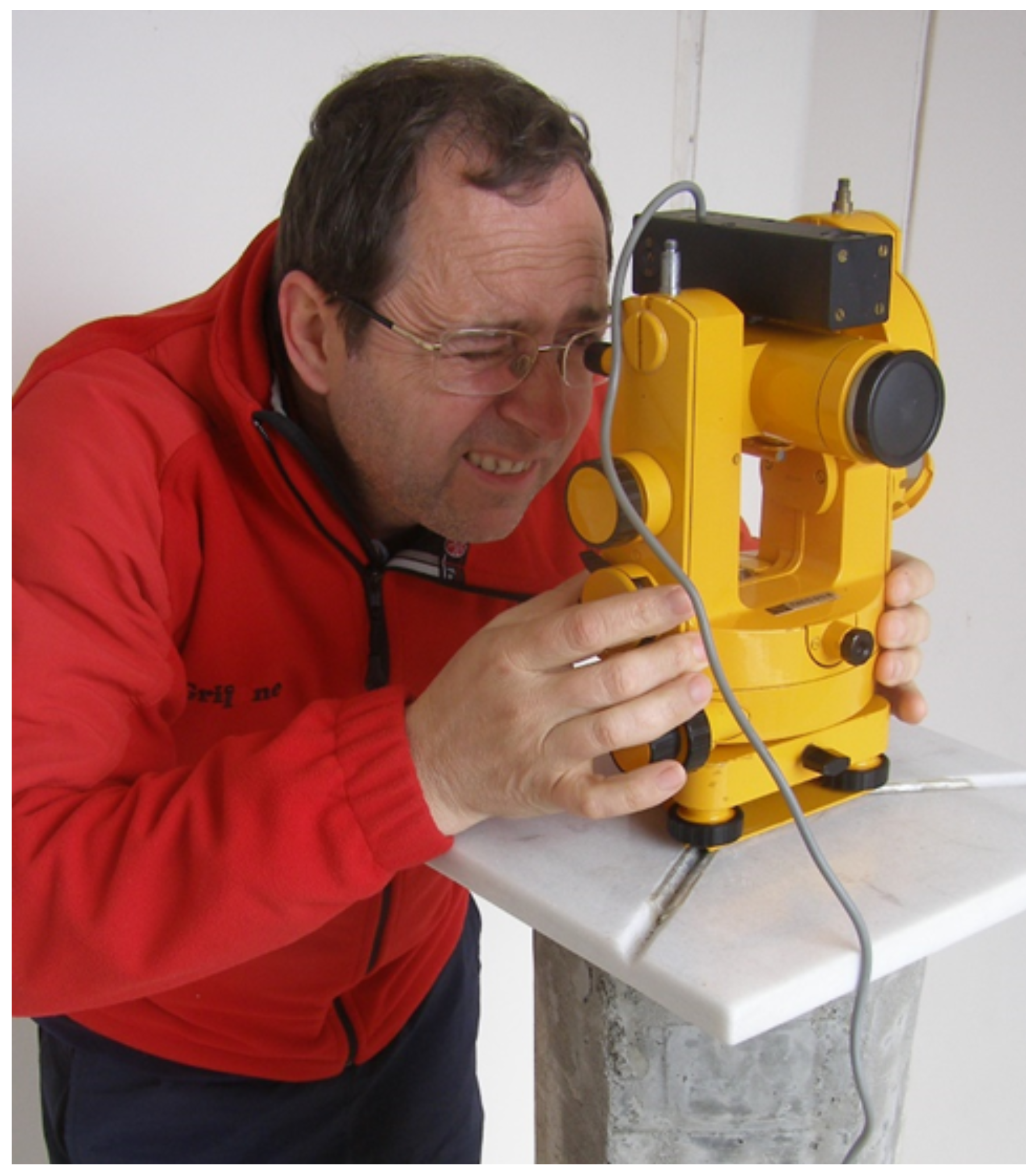
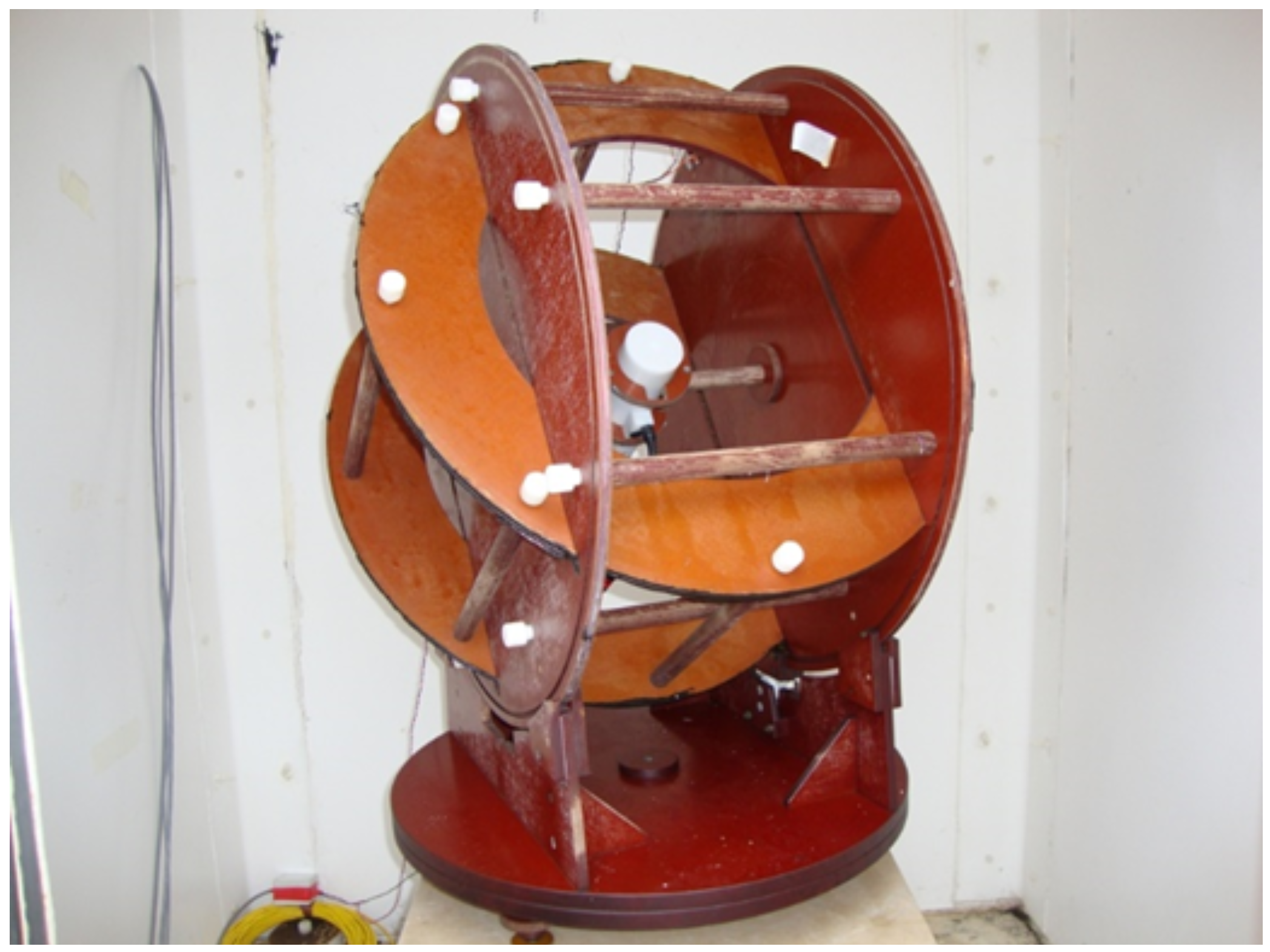
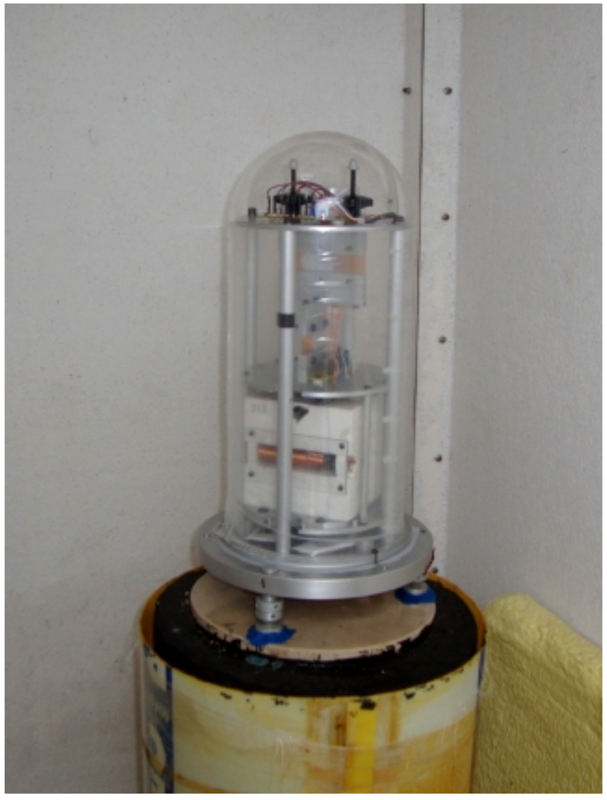
2.1. Measurements of Geomagnetic Parameters

Measuring geomagnetic parameters is a complex task due to the fact that the physical magnitude to be measured is a vector. This requires an accurate determination of the magnitudes with respect to a fixed reference frame and skilled staff from both technical and scientific points of view.

The geomagnetic vector can be given in either of three coordinate systems based on a geographic reference: (i) Cartesian, where X, Y, Z are the geographic north, east and altitude projections, respectively; (ii) cylindrical, where H and Z are the horizontal and altitude projections and D is the declination angle between the geographic north and the magnetic field, establishing that the positive is towards east; and (iii) spherical, where F is the total vector magnitude, D is the declination and I is the inclination angle between the horizontal projection and the magnetic vector itself, establishing the positive downwards.

As far as the geomagnetic sensors are concerned, a D/I fluxgate theodolite (see Figure 2) is mounted in the first hut of the ASJI. This sensor permits a manual measurement of the declination and inclination angles of the vector magnetic field in absolute terms, which permits one to discuss the uncertainties of this instrument [10]. It consists of a fluxgate magnetometer bar mounted on the telescope of a non-magnetic theodolite.

Figure 2. The manual declination and inclination (D/I) fluxgate theodolite being manipulated by a specialist. More details about the sensor can be found in [9].

Figure 2. The manual declination and inclination (D/I) fluxgate theodolite being manipulated by a specialist. More details about the sensor can be found in [9].

A variometer type δD/δI vector magnetometer (see Figure 3) is mounted in the second hut to measure the variations of the magnetic field vector automatically once per minute. It consists of two perpendicular pairs of Helmholtz coils, the polarization of which allows measuring the declination and inclination variations with a proton magnetometer located at their center [11]. The proton magnetometer measures the total magnetic field intensity, F, when the coils are not polarized.

Figure 3. δD/δI vector magnetometer deployed at the ASJI with the two perpendicular pairs of Helmholtz coils and the proton magnetometer allowing one to measure the variations of D/I. More details about the sensor can be found in [9].

Figure 3. δD/δI vector magnetometer deployed at the ASJI with the two perpendicular pairs of Helmholtz coils and the proton magnetometer allowing one to measure the variations of D/I. More details about the sensor can be found in [9].

The last of these three huts houses the electronic system controlling this automatic instrument. A new three-axis fluxgate magnetometer (see Figure 4) was added during the 2008 expedition. It is able to measure the magnetic field variations automatically from an analogue output sampling at both 1 and 0.1 Hz by the corresponding analog to digital converter (ADC).

Figure 4. The three-axis automatic fluxgate magnetometer was added in 2008. More details about the sensor can be found in [9].

Figure 4. The three-axis automatic fluxgate magnetometer was added in 2008. More details about the sensor can be found in [9].

Once the raw data are processed, the definitive dataset is sent to the World Data Centers, becoming accessible to the scientific community. Nowadays, real-time access to the data is provided through a satellite link thanks to the International Real-time Magnetic Observatory (INTERMAGNET). Nevertheless, a reliable skywave link designed by La Salle and the Ebro Observatory is active as a backup. A future project is motivated to separate our sensor data from the INTERMAGNET link and to transmit only through the autonomous skywave link, which, besides, is becoming another interesting sensor of the ionosphere due to the capability of measuring the ionosphere’s performance.

2.2. Vertical Incidence Soundings of the Ionosphere

A vertical incidence ionospheric sounder (VIS) was installed at the ASJI (Figure 5) during the 2004 to 2005 survey to provide information about the ionospheric characteristics in this region. Data provided by the VIS are used to characterize the climatology of the ionosphere and to investigate the ionospheric effects caused under geomagnetically-disturbed periods.

The VIS located at the ASJI records a vertical incidence ionogram every 10 min. An ionogram is a graph that represents the time-of-flight for every radio frequency transmitted vertically and received after its reflection in the ionosphere. Figure 6 shows an example of a ionogram recorded by the VIS at the ASJI where the particular layers of the ionosphere can be seen clearly. For more details about the VIS soundings, see [13].

Figure 5. The vertical incidence ionospheric sounder (VIS) installed at the ASJI is the Advanced Ionospheric Sounder (AIS) developed by the Instituto Nazionale di Geofisica e Vulcanologia (INGV) of Rome, Italy. For more details about the ionosonde, see [12].

Figure 5. The vertical incidence ionospheric sounder (VIS) installed at the ASJI is the Advanced Ionospheric Sounder (AIS) developed by the Instituto Nazionale di Geofisica e Vulcanologia (INGV) of Rome, Italy. For more details about the ionosonde, see [12].

Figure 6. An example of an ionogram recorded by the VIS at the ASJI where one can see clearly the particular layers of the ionosphere.

Figure 6. An example of an ionogram recorded by the VIS at the ASJI where one can see clearly the particular layers of the ionosphere.

Oblique Incidence Soundings of the Ionosphere

The oblique ionosonde is developed by La Salle to analyze and characterize the ionospheric channel between Antarctica and Spain [4]. It is used to obtain useful and key parameters for modeling the HF radio link; i.e., link availability, power delay profile of the channel and frequency dispersion. The soundings are carried out during the austral summer, when the ASJI is operative; the transmitter antenna is located at the ASJI (see Figure 7), and the receiver is located in Cambrils, Spain. More details of the HF data transmission are given in Section 4.

Figure 7. The antenna of the oblique ionosonde transmitter at the ASJI.

Figure 7. The antenna of the oblique ionosonde transmitter at the ASJI.

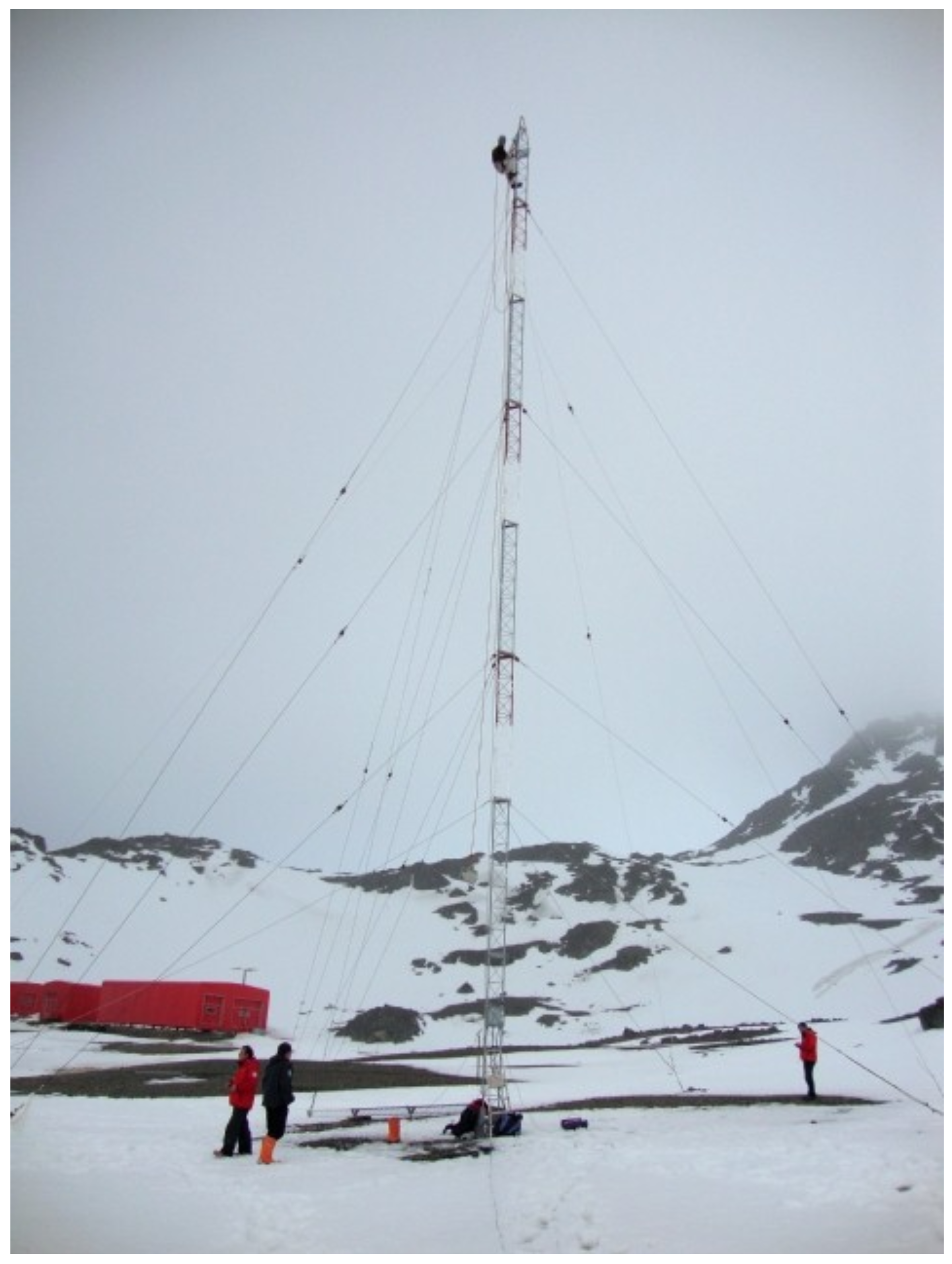
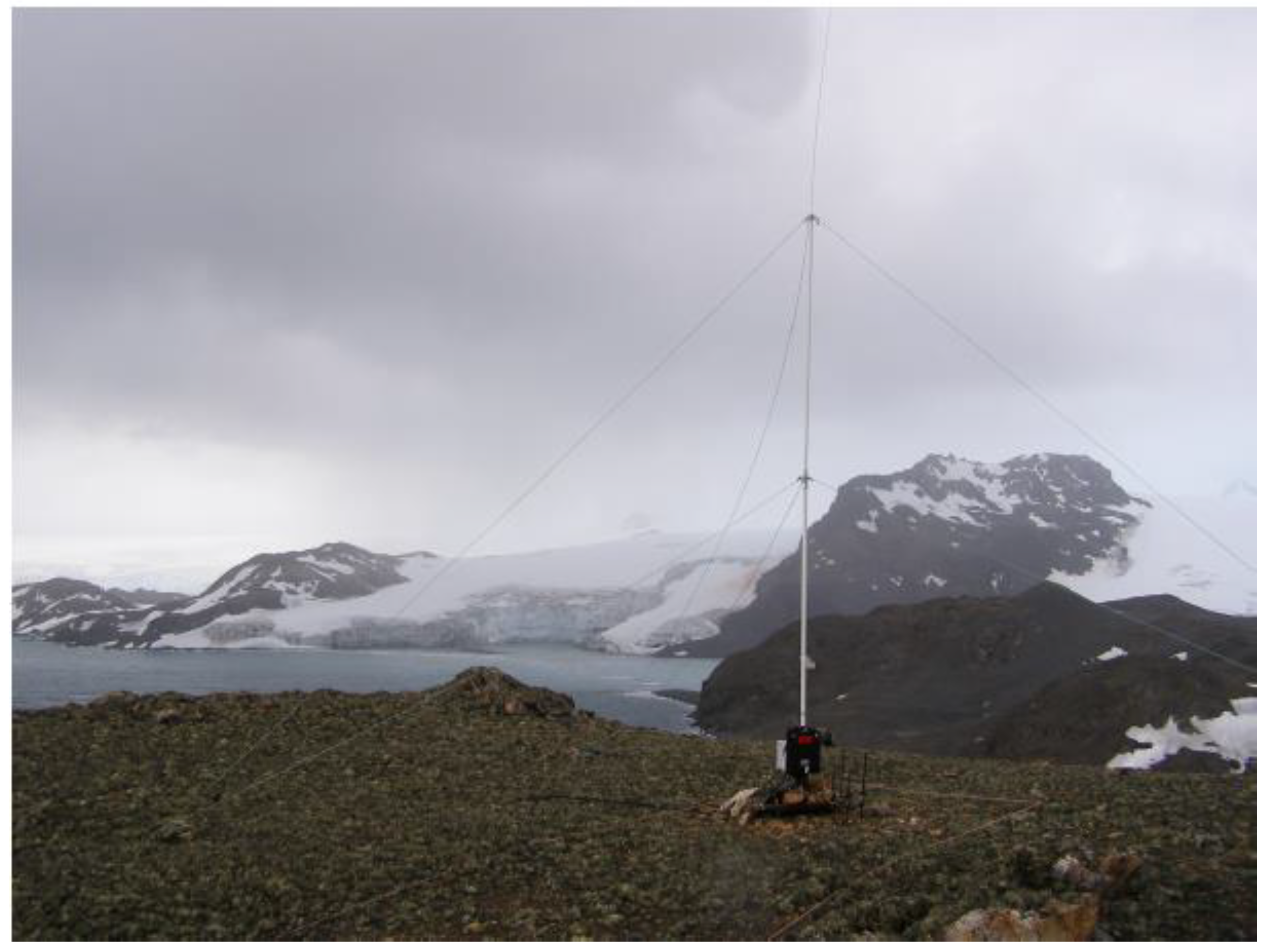
3. System Description

The hardware of the ionospheric channel sounder jointly with the oblique ionosonde and data transmission system has been designed in order to have an extended frequency range and to get the best frequency and time accuracy. Moreover, the whole transmission system has been entirely redesigned from the initial system deployed on the survey of 2003 to 2004 [4]. It was upgraded with faster and more reliable equipment during the 2009 to 2010 expedition. As a result of the last improvement, the system is able to operate at a higher bandwidth up to 40 kHz and to sample at 100 ksps. Furthermore, the system was redesigned to be more flexible concerning the frequency and bandwidth selection for the soundings.

The main features of the transmitter and receiver hardware are described below.

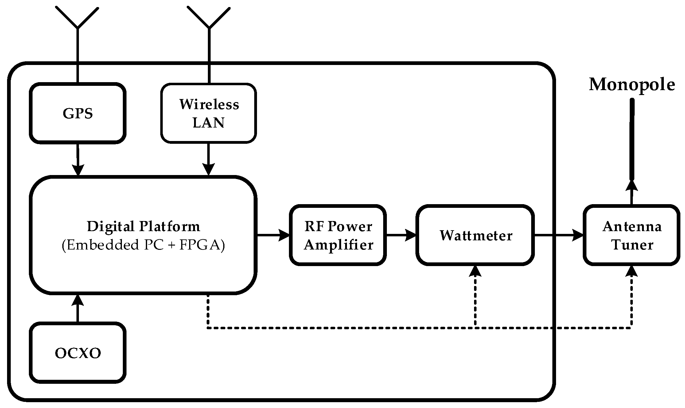
3.1. Hardware of the Transmitter

The core is composed of an embedded PC with a digital signal processing (DSP) unit inside, which performs the tasks of controlling and configuring the system parameters. The main DSP unit is the XTremeDSP-IV from Nallatech, and it includes three Xilinx FPGA1s described below: (i) a Virtex-II is responsible for clock configuration; (ii) a Spartan-II handles the interface between the PCI bus; and (iii) a Virtex-4, which performs the software radio procedures. In order to perform these software radio operations, the Virtex-4 is equipped with two 14-bit ADC, two 14-bit DAC and all of the arithmetic and peripheral drivers. Figure 8 shows a block diagram of the transmitter.

Moreover, a GPS unit is placed to make the time synchronization possible using the pulse per second (PPS) signal, which makes it possible to measure the propagation time of the wave with an accuracy of 1 μs. Furthermore, a 100-MHz oven controlled crystal oscillator (OCXO) is installed in both the transmitter and receiver in order to increase the frequency synchronization accuracy. The Wattmeter measures the forward and reverse transmitted power in order to notice severe impedance mismatch. Additionally, the FPGA is capable, thanks to its peripheral drivers, of switching off the amplifier in case of malfunctioning. The antenna tuner is used to semi-automatically tune the monopole antenna, which transmits the signal.

As far as the deployment is concerned, all of the transmitter hardware is close to the antenna at the top of a hill near the ASJI. All of the electronics are sealed inside a watertight box, which protects against severe weather conditions and provides electromagnetic shielding. The system is remotely accessed through a wireless local area network (WLAN) from the laboratory at the ASJI.

Figure 8. Scheme of the transmitter that consists of an embedded digital platform and different peripherals used to control the system and to improve the synchronization.

Figure 8. Scheme of the transmitter that consists of an embedded digital platform and different peripherals used to control the system and to improve the synchronization.

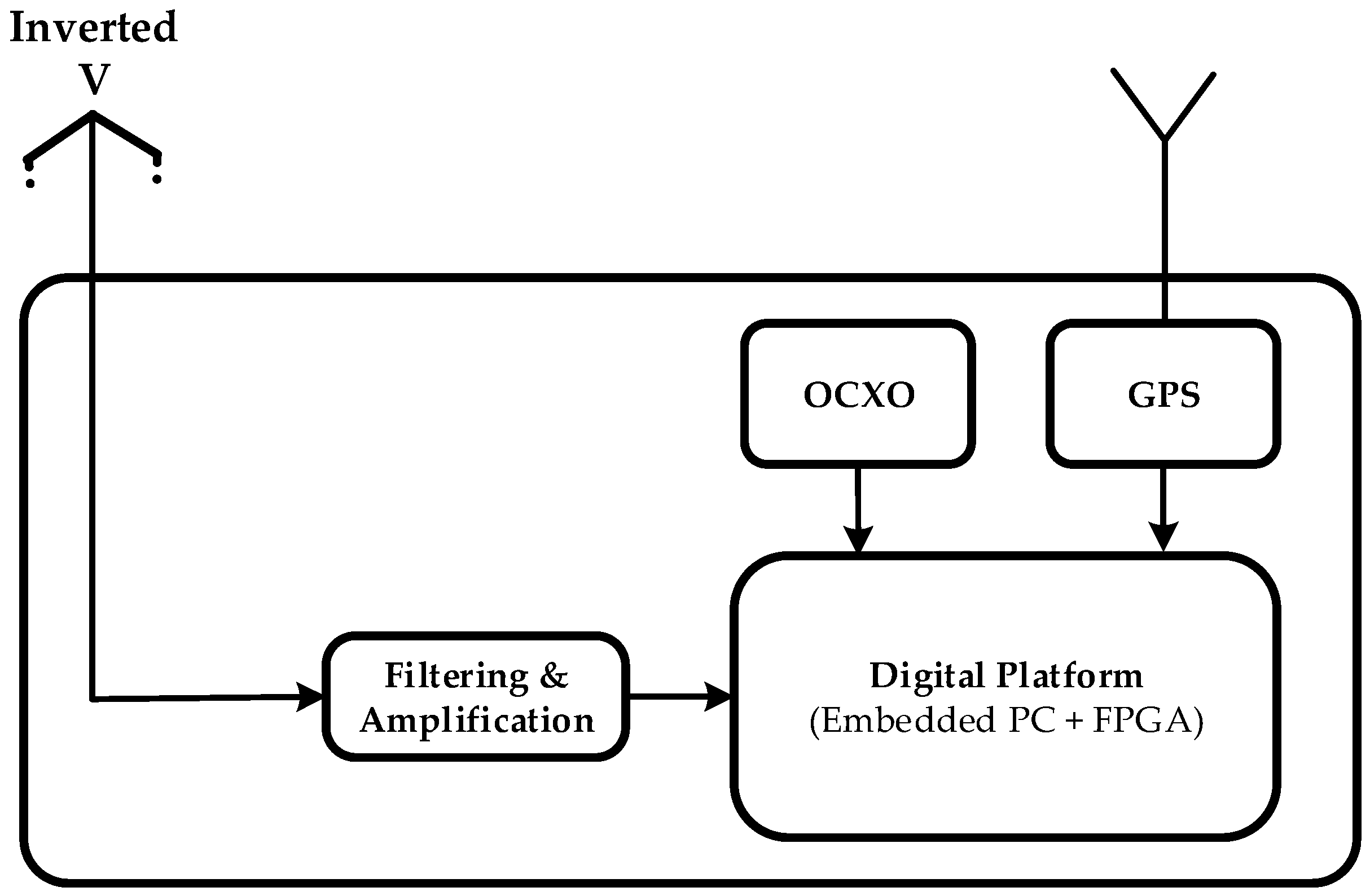
3.2. Hardware of the Receiver

An inverted-V antenna is used to obtain the signal for the receiver. As shown in Figure 9, the radio frequency signal is passed through a certain filtering and amplification process and given next to the digital platform, which works the same way as the transmitter described above. Moreover, the receiver also has an OCXO and a GPS to improve both frequency and time synchronization. A block diagram of the receiver is shown in Figure 9.

Figure 9. Scheme of the receiver that consists of several filtering stages and a digital platform with peripherals to improve synchronization.

Figure 9. Scheme of the receiver that consists of several filtering stages and a digital platform with peripherals to improve synchronization.

4. Data Analysis

This section presents a detailed explanation of the test description and the analysis algorithms for narrowband and wideband oblique sounding.

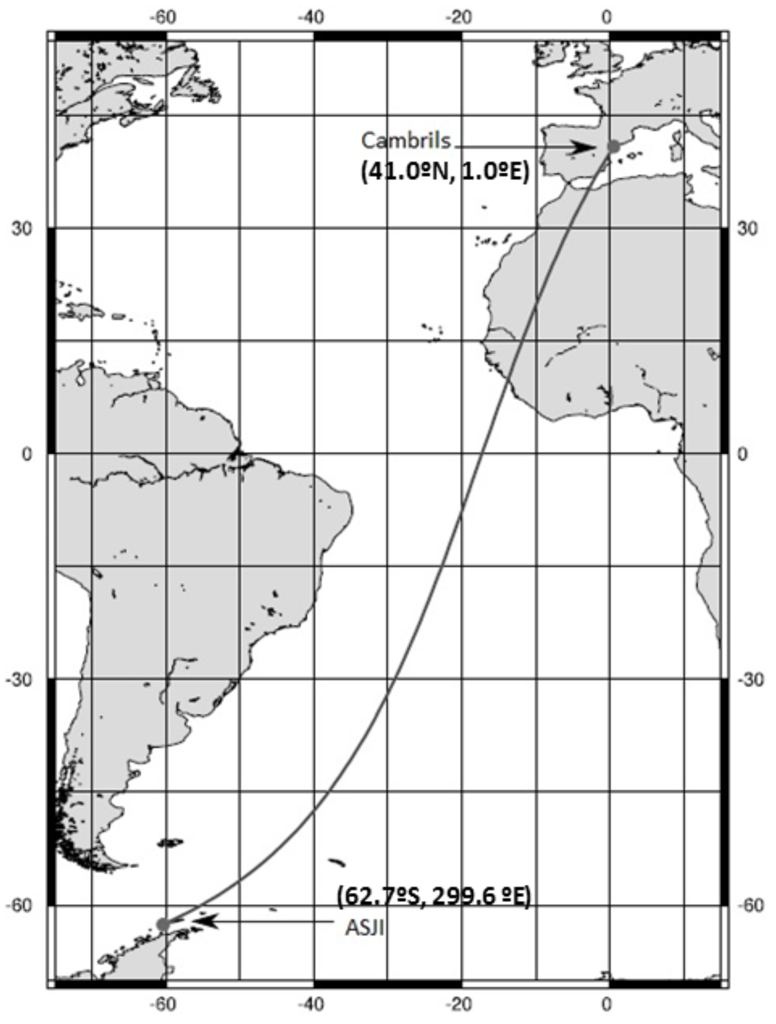
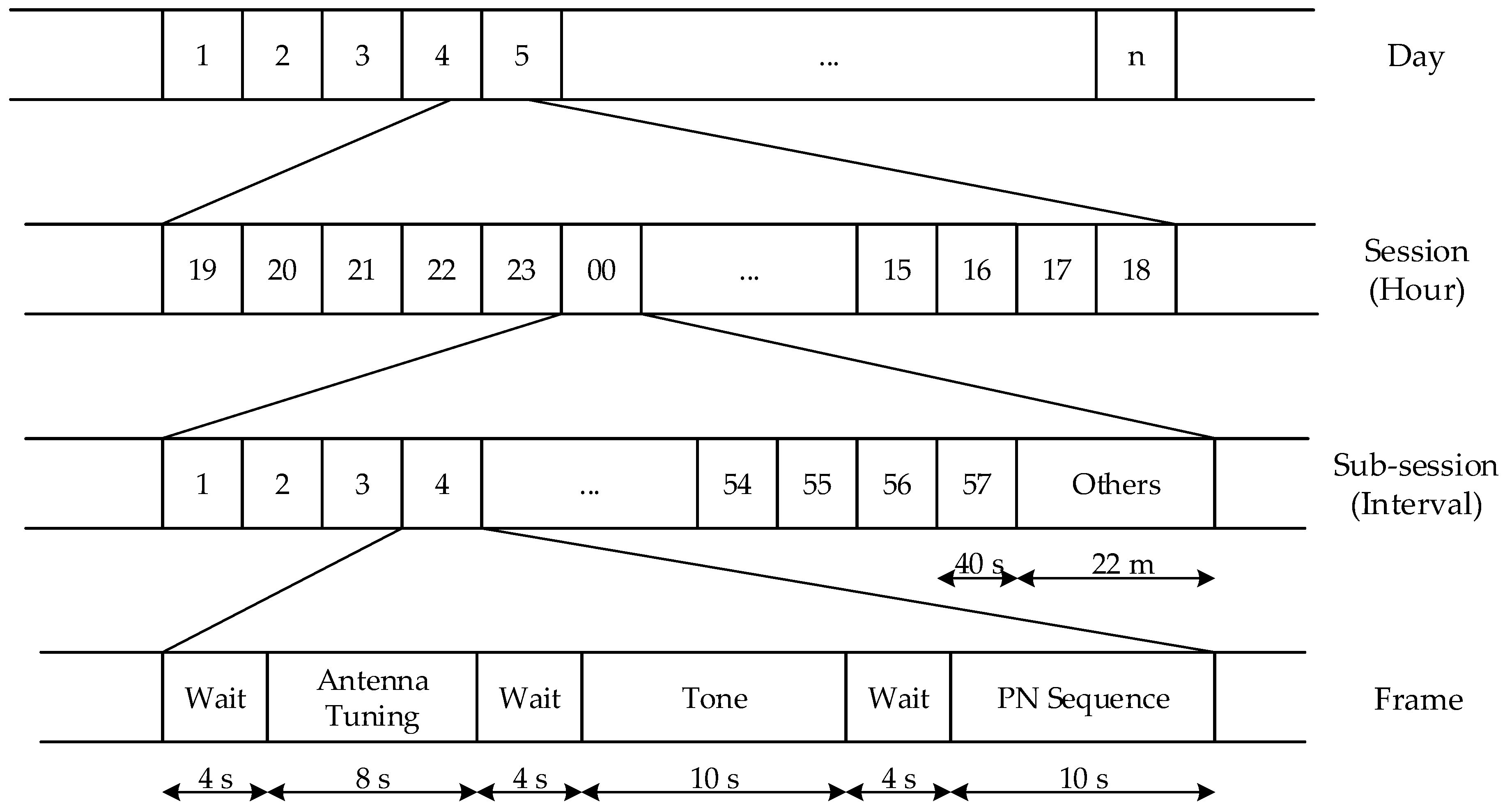
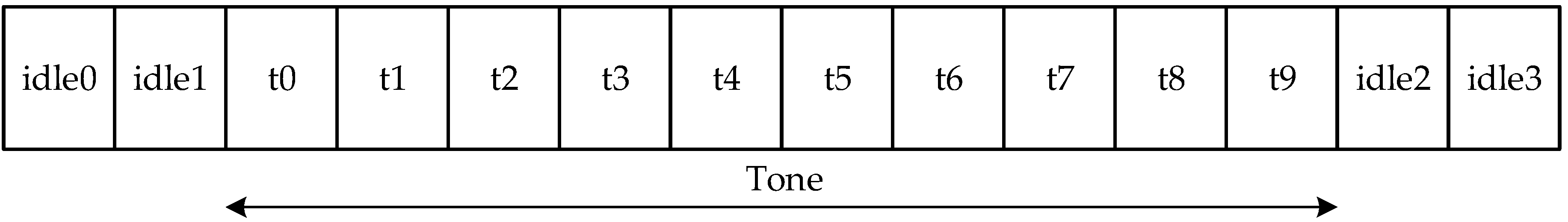
4.1. Tests Description

The analysis of the sounding channel has been carried out in both narrowband and wideband. While the narrowband analysis focuses on channel availability and the signal-to-noise ratio (SNR), the wideband calculates the scattering function from the estimated channel impulse response and then evaluates the multipath delay spread and Doppler spread.

The soundings are carried out during 24 h a day (sessions) for a frequency carrier ranging from 2 to 30 MHz with steps of 500 Hz, which corresponds to 57 sub-sessions. Every sub-session is divided into a frame to subdivide the time into two experiments, using 40 s for both of them. Finally, every session has a time slot of 22 min (called “others” in the figure) to transmit the data from the sensors and to test also new modulations schemes. The structure of the periodic experiment conducted during the 2013 to 2014 campaign is described in Figure 10. These soundings were carried out for 25 days, between 25 January and 18 February.

The idle intervals are included in all frames to ensure the system synchronization. The smart antenna tuning works around 20 W, and it is required because the transmitter antenna is a monopole (so, it requires tuning for each frequency). The channel sounding is carried out in the processes called “tone” and “pseudonoise (PN) sequence” during 10 s each.

Figure 10. Frame structure of the channel sounding.

Figure 10. Frame structure of the channel sounding.

The narrowband analysis is necessary to characterize the channel in terms of SNR and availability, using a sine wave as the transmitted signal. This tone is transmitted during 10 s. The configuration parameters are detailed in Table 1.

Table 1. Configuration parameters and setup for the narrowband sounding in the 2013 to 2014 survey.

Parameter	Value
Signal	Sine wave
Duration	10 s
Silence	4 s

Table 1. Configuration parameters and setup for the narrowband sounding in the 2013 to 2014 survey.

Parameter	Value
Signal	Sine wave
Duration	10 s
Silence	4 s

The wideband analysis is necessary to characterize the time and frequency dispersion in the channel. The transmitted signal for the wideband analysis is a PN sequence [14] with the configuration parameters detailed in Table 2.

Table 2. Configuration parameters and setup for the wideband sounding in the 2013 to 2014 survey.

Parameter	Value
Sampling frequency	100 kHz
PN sequence length	127
Family of sequences	m-sequence
Chip frequency	5 kHz
Number of sequences per test	300

Table 2. Configuration parameters and setup for the wideband sounding in the 2013 to 2014 survey.

Parameter	Value
Sampling frequency	100 kHz
PN sequence length	127
Family of sequences	m-sequence
Chip frequency	5 kHz
Number of sequences per test	300

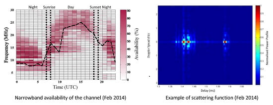
4.2. Narrowband Analysis

The narrowband analysis focuses on SNR and channel availability computation. The channel availability is defined as the probability of a link to reach a minimum SNR value and, therefore, achieving a certain quality of service (see [15] for more details). A minimum SNR value of 6 dB was specified to estimate the channel availability in a bandwidth of 10 Hz [4]. In order to improve the reliability of the detection system, due to the probability of high noise and interference, several techniques were developed in [5]. SNR is computed with the comparison between the received power measured during the tone intervals and the noise power measured during the idle periods.

The first step is to filter the signal to obtain a usable power profile, conducted in the frequency domain with the fast Fourier transform (FFT). Afterwards, a windowing is applied to: (i) remove the non-desirable signals from the reception frequency (which changes from 2 MHz to 30 MHz in the soundings); and (ii) avoid creating transients from the impulsive interferences falling far away from the reception frequency when an ideal filter is used. Previous tests showed that the Kaiser window presents a better, smoother response [5].

The measurements of SNR can be distorted easily because of the high level of interferences. To overcome this problem, a time framing technique is used, consisting of dividing the tone interval into the 10 smallest sub-intervals of 1 s each and observing the evolution of the SNR along the whole interval (see in Figure 11).

Figure 11. Diagram of time framing technique for narrowband sounding.

Figure 11. Diagram of time framing technique for narrowband sounding.

According to previous experiments, two SNR threshold values are defined, Th_Low = 3dB and Th_High = 6dB. Only those measurements that fulfill SNR ≥ Th_Low over 70% of the segments or SNR ≥ Th_High over 60% of the segments are taken into account to estimate the SNR and channel availability. An estimation of the SNR result of 17 February is shown in Figure 12.

Figure 12. SNR of 17 February (in dB) over a bandwidth of 10 Hz, in which the regions of day, night and the time just after sunrise and the time just after sunset can be appreciated.

Figure 12. SNR of 17 February (in dB) over a bandwidth of 10 Hz, in which the regions of day, night and the time just after sunrise and the time just after sunset can be appreciated.

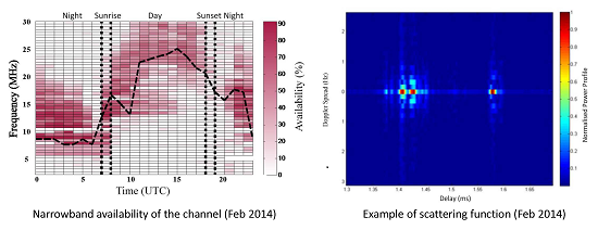
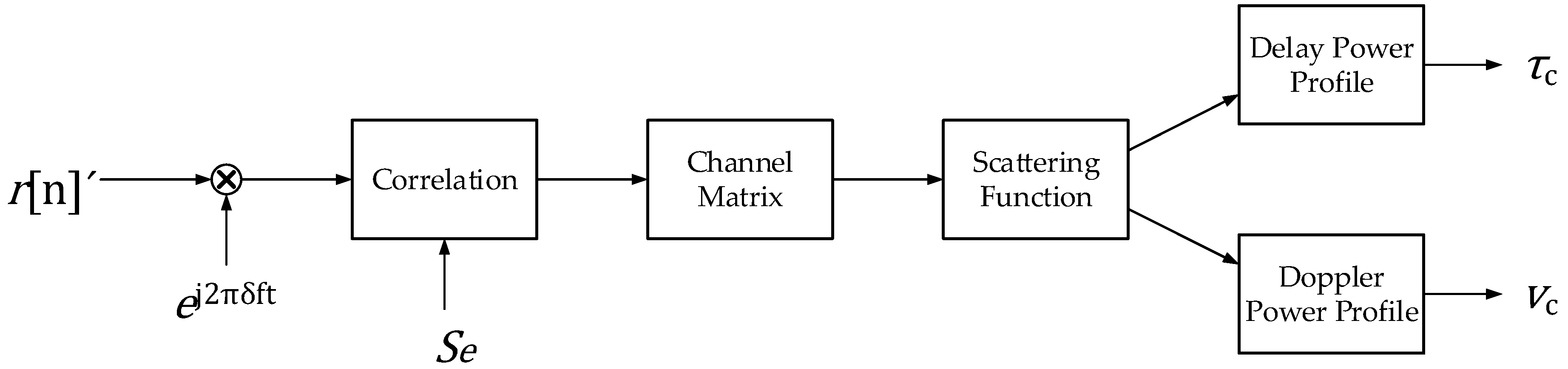
4.2.1. Wideband Analysis

The wideband analysis is performed sending PN waveforms with good cyclic cross-correlation characteristics, therefore using M-sequences [16]. The computation process for the wideband sounding is detailed in Figure 13.

Figure 13. Diagram of the computation process for wideband channel sounding.

Figure 13. Diagram of the computation process for wideband channel sounding.

The wideband analysis is crucial to characterize time and frequency dispersion in the channel. First, the received signal r[n] (with the characteristics described in Section 4.1) is correlated with the original PN sequence Se. The correlation function is calculated as:

$${\mathrm{\varphi }}_{r,S_e}\left[n\right]={\displaystyle \sum _{k=0}^{N_e-1}}r[n+k]S_e\left[k\right]$$

(1)

where N_e is the length of the PN sequence. Hence, the channel impulse response h[n, τ] can be written as:

$$h[n,\mathrm{\tau }]={\mathrm{\varphi }}_{r,S_e}[nl{N}_c+\mathrm{\tau }]$$

(2)

where τ is the delay variable, l is the number of chips and N_c is the number of samples per chip. From Equation 2, the following parameters are calculated: scattering function, composite multipath spread and composite Doppler spread. The scattering function R_s[τ, v] is calculated as the FFT of the channel impulse response [16].

$$R_h[\xi ,\mathrm{\tau }]={\displaystyle \sum _{\xi }}{h}^{*}[n,\mathrm{\tau }]h[n+\xi ,\mathrm{\tau }]$$

(3)

$$R_s[\mathrm{\tau },v]={\displaystyle \sum _{\mathrm{\xi }}}{R}_h[\xi ,\mathrm{\tau }]e^{-j2\pi \xi v}$$

(4)

Both the composite multipath spread and the composite Doppler spread are calculated from the data obtained in the scattering function R_s[τ, v]]. Let [τ₁, τ₂] be the multipath observation window and [v₁, v₂] the Doppler spread observation window. Consequently, both multipath power profiles are defined as:

$$\mathrm{\varphi }\left[\mathrm{\tau }\right]={\displaystyle \sum _{v=v_1}^{v_2}}{R}_s[\mathrm{\tau },v]$$

(5)

and the Doppler power profile is defined as:

$$\mathrm{\varphi }\left[v\right]={\displaystyle \sum _{\mathrm{\tau }={\mathrm{\tau }}_1}^{{\mathrm{\tau }}_2}}{R}_s[\mathrm{\tau },v]$$

(6)

In this work, the windows have been set to [−3.5, 3.5] (ms) and [−2.5, 2.5] (Hz), respectively, due to the maximum delay and Doppler spread values obtained in previous tests [4]. Next, the spread parameters are calculated. The multipath spread is measured from the multipath power profile as 80% of the power spread [4]. This parameter is named the composite multipath spread (t_eff) and was defined in [17]. In the same way, the Doppler spread is measured from the Doppler power profile as the 80% power spread. It is named composite Doppler spread (u_eff), and it was defined in [20]. In Figure 14, we can observe the performance of the wideband sounding of 1 February 2014, at 00 UTC for 13 MHz of carrier frequency. In Figure 14a, the channel response h[n, τ] is plotted, and the channel variations with time can be observed. In Figure 14b, the scattering function has been calculated using h[n, τ], and R_s[τ, v] is obtained after performing the FFT. In Figure 14c, the multipath power profile is observed for the previously-defined time window, and finally, in Figure 14e, the Doppler power profile is plotted for the previously-defined frequency window.

Figure 14. Wideband channel response and measures for 1 February 2014 at 07 UTC with 13 MHz of carrier frequency: (a) normalized channel response h[n, τ]; (b) normalized scattering function R_s[τ, v]; (c) multipath power profile (in ms); (d) the integral of the multipath power profile to calculate the delay spread (in ms); (e) Doppler power profile (in Hz); and (f) the integral of the Doppler power profile to calculate the Doppler spread (in Hz).

Figure 14. Wideband channel response and measures for 1 February 2014 at 07 UTC with 13 MHz of carrier frequency: (a) normalized channel response h[n, τ]; (b) normalized scattering function R_s[τ, v]; (c) multipath power profile (in ms); (d) the integral of the multipath power profile to calculate the delay spread (in ms); (e) Doppler power profile (in Hz); and (f) the integral of the Doppler power profile to calculate the Doppler spread (in Hz).

Finally, the last of the wideband analyses is the number of paths, which is defined as follows. The number of paths is measured comparing the number of paths found at two energy levels in terms of the percentage of the maximum; the final number chosen is the higher value measured. The two thresholds are settled in 70% and 45% of the maximum value corresponding to the strongest path. With this method, the system evaluates the maximum number of paths, taking into account both the strongest ones and the weakest ones. The two thresholds were settled testing the results over the data, measuring which levels of energy determined the more realistic result depending on the channel response. In Figure 15, both thresholds are settled, and two different measures are obtained: the 70% one detects one path, and the 45% threshold detects two paths. Neither of the two detects the third small path in between, but the lower value could not be made smaller, as this would lead to confusion in the case of a noisy environment.

Figure 15. Example of channel response and the measure of the number of paths on the 70% and on the 45% threshold. The first one only detects one path, and the second one detects two paths. None of them detect the third small path.

Figure 15. Example of channel response and the measure of the number of paths on the 70% and on the 45% threshold. The first one only detects one path, and the second one detects two paths. None of them detect the third small path.

5. Results

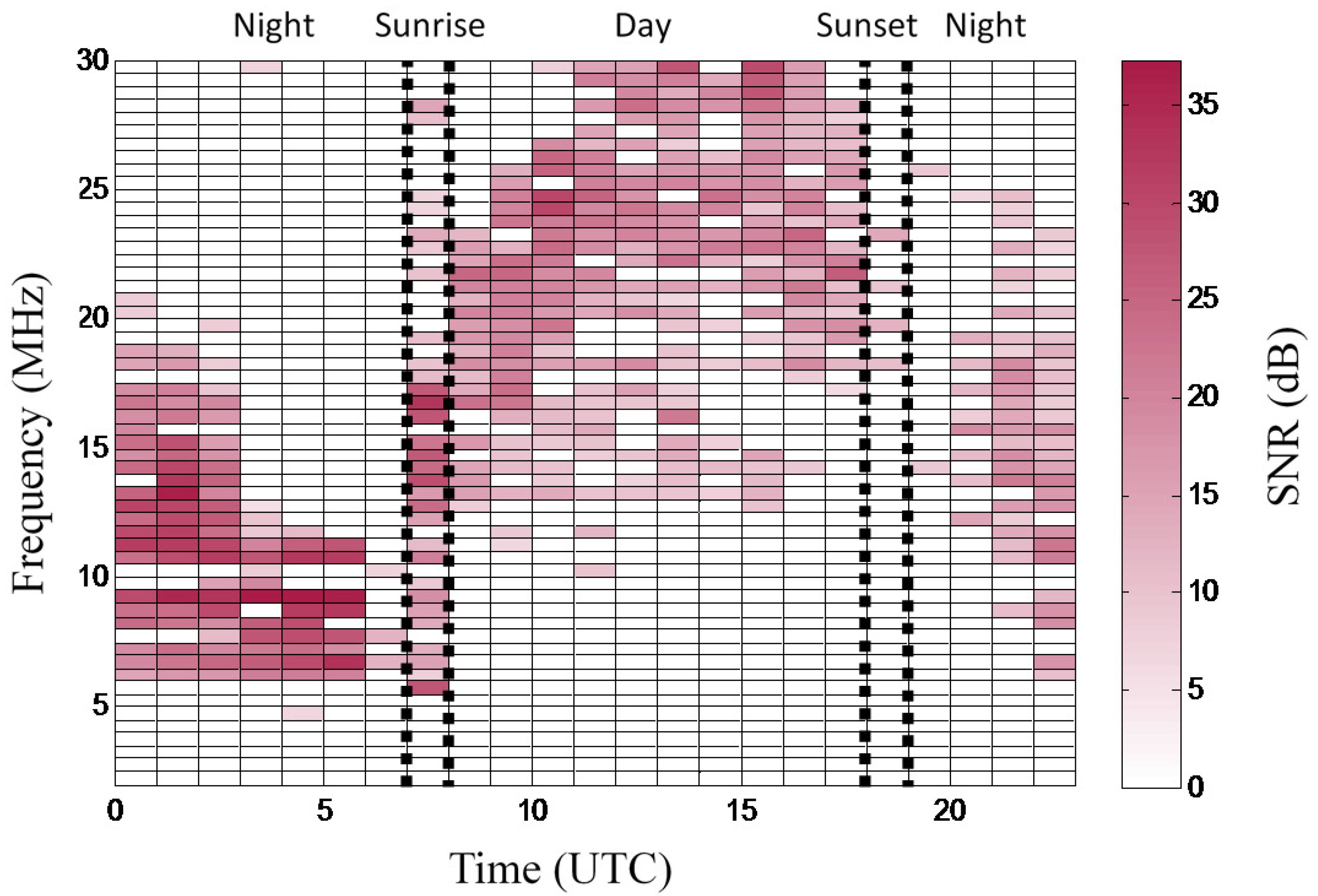
5.1. Narrowband Results

The results of narrowband analysis shown in Figure 16 represent the average plot of the channel availability for the survey. Figure 16 depicts the channel availability for frequencies ranging from 2 to 30 MHz as a function of time. The frequency of largest availability (FLA) for a particular time is shown as a dashed line. Four different zones can be distinguished: day, night, sunrise and sunset. During the day interval, from 08 UTC to 17 UTC, the frequencies ranging from 20 to 30 MHz present the better performance in terms of SNR. For the sunset period, around 18 UTC, the interval of frequencies that performs best falls linearly with the time between 20 and 30 MHz to 10 and 20 MHz. The night period is defined from 19 UTC to 06 UTC, and the frequencies ranging from 6 to 15 MHz show the best results. Finally, for the sunrise, which is the period defined around 07 UTC, its best operation frequencies increase linearly with the time from frequencies between 6 and 15 MHz to frequencies ranging from 20 to 30 MHz. As a consequence, we can conclude that the best reflective frequencies during the daytime are the highest frequency range, the nighttime the lowest one, and sunrise and sunset are regions of switching between these periods of time performing in an unstable condition for all frequencies. It is worth noticing a drop in the FLA after sunrise (9 to 10 UT) and a post sunset jump (20 to 21 UT) of the FLA. These effects deviate from the expected smooth transition of the FLA from nighttime to daytime conditions and vice versa [18,19]. These effects will be studied in future analyses.

Figure 16. Channel availability of the campaign of 2014 measured during the austral summer, from 25 January to 18 February.

Figure 16. Channel availability of the campaign of 2014 measured during the austral summer, from 25 January to 18 February.

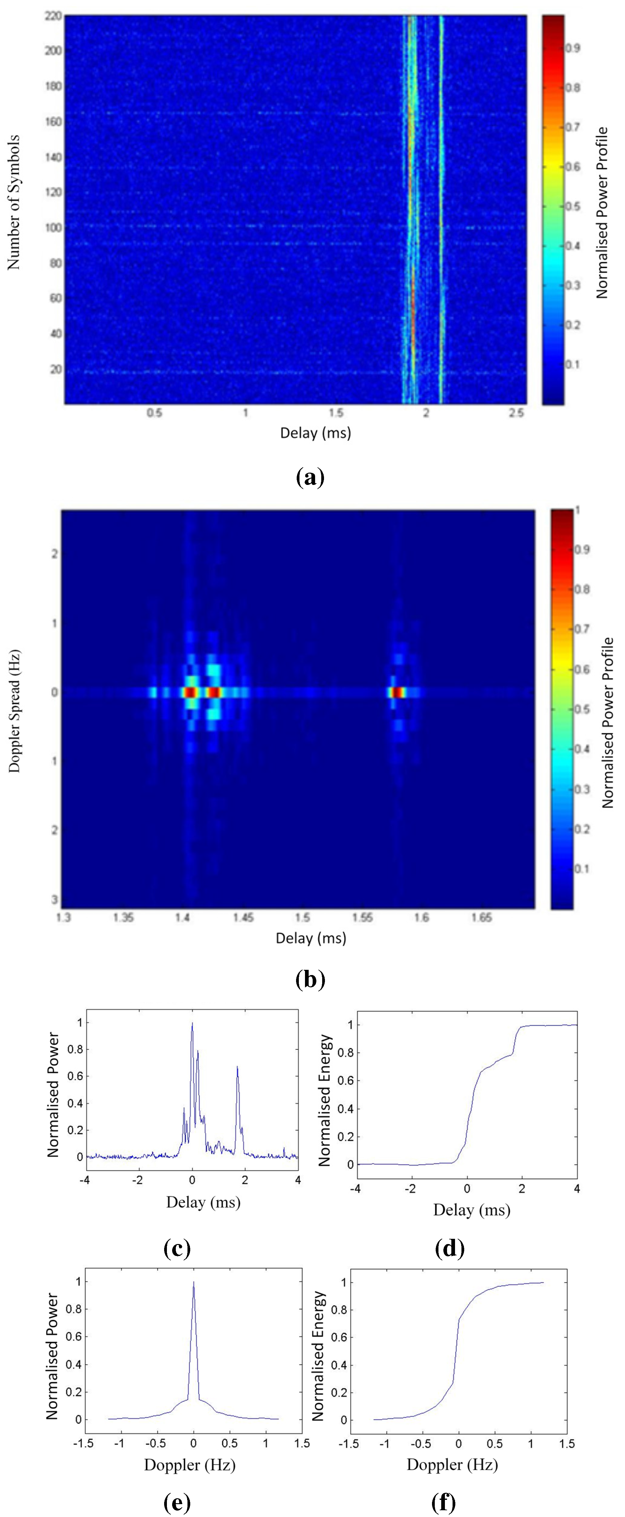
5.2. Wideband Results

The results of wideband analysis are shown in Figure 17, containing the delay spread, the Doppler spread and the number of paths.

Figure 17a,c present the mean delay spread and the mean Doppler spread, from which one can distinguish four different performance zones also: day, night, sunrise and sunset [17]. Figure 17b,d show the standard deviation for the delay spread and the Doppler spread, respectively. During the day interval, from 08 UTC to 17 UTC, high frequencies ranging from 20 MHz to 30 MHz show the higher delay spread and Doppler spread for all measures. This means that the channel is available for a wide range of frequencies, but its channel response is varying and unstable; additionally, the intersymbol interference caused by a long channel response is an important parameter for the modulation design. Sunset time, around 18 UTC, presents an irregular performance when comparing high frequencies and low ones, but low frequencies start performing better, while high frequencies decrease its availability. Furthermore, sunrise, around 07 UTC, shows unstable performance in terms of wideband availability. Nighttime, shown both on the right and on the left of Figure 17, ranging from 19 UTC to 06 UTC, presents the best measurements in terms of channel availability and parameters. The best frequencies are around 10 MHz, despite the channel being available until 20 MHz. Delay spread mean values are around 2 or 3 ms, with low deviation, and maximum Doppler spread values are around 0.7 Hz. All of this information is compared to Figure 17e,f, which shows the number of paths calculated in the channel response. The number of paths is a difficult parameter to evaluate, depending on the energy level threshold to consider a new path. The number of paths in this study is calculated by evaluating the number of countable paths in both 70% of the maximum and in 45% of the maximum, saving the highest value. During the day hours, from 08 UTC to 17 UTC, the lower number of paths is shown. Both for sunrise and for sunset, it shows unstable performance in terms of the number of paths. Finally, the number of paths during the night reaches its highest levels, showing good propagation through several different channel lengths.

Figure 17. Wideband channel measurements during the campaign of 2014: (a) mean of delay spread (in ms); (b) standard deviation of delay spread (in ms); (c) mean of Doppler spread (in Hz); (d) standard deviation of Doppler spread (in Hz); (e) mean of the number of paths; and (f) standard deviation of the number of paths.

Figure 17. Wideband channel measurements during the campaign of 2014: (a) mean of delay spread (in ms); (b) standard deviation of delay spread (in ms); (c) mean of Doppler spread (in Hz); (d) standard deviation of Doppler spread (in Hz); (e) mean of the number of paths; and (f) standard deviation of the number of paths.

5.3. Discussion

The narrowband and wideband analyses conducted show similar results in terms of availability depending on the hour of the day. Nighttime is the best reception time, using frequencies from 8 MHz to 20 MHz. Narrowband presents its best SNR results, while wideband shows its smaller delay spread and Doppler spread measurements.

The results obtained show similar performance as found in [4], but our analyses with the 2014 campaign can be done in a more precise way thanks to the change of the transmitter and the receiver system [5], as well as the higher number of sounding frequencies and hours of the day. Therefore, our previous soundings, performed with less detail, have been confirmed by the results of the analysis of the 2014 campaign.

These parameter results, together with our previous modulation studies [6,7], allow us to conclude that for the best hours and frequencies, high throughput modulations, like OFDM, should be used, in order to increase the bit rate of the communication. Delay spread and Doppler spread will not worsen the results in a severe way, according to the measured values. Despite that, the OFDM modulation should be designed taking into account the coherence time and coherence bandwidth calculated using the measured parameters of the Doppler spread and the delay spread. Finally, for sunrise, sunset and daytime, a more robust modulation should be used. The direct-sequence spread spectrum (already analyzed in [7,8]) could be a good option, assuming lower throughput, but ensuring a more robust communication against channel variations or fadings.

6. Conclusions

This paper presents the main results of the oblique sounding measurement recorded during the campaign of 2014 with a transmitter placed at the Remote Geophysical Observatory of the ASJI and the receiver located in Cambrils (Spain). The sounding has been carried out for both narrowband and wideband to characterize the channel in terms of SNR, availability, multipath delay spread, Doppler spread and number of paths. These measurements of the long haul link improve the knowledge of the performance of the ionospheric channel that is 12,760 km long, together with previous work [4,5]. They also allow us, taking into account previous works on modulations [6,7,8], to complete the full definition of the physical layer to send the data of the remote sensors deployed across the island from Antarctica to Spain.

The values measured for narrowband and wideband confirm that both soundings show similar results in terms of availability depending on the hour of the day and of the frequency used. Furthermore, the wideband analysis presents the results of the period of the day that is more suitable for data transmission, because the channel shows a good performance (with low Doppler spread and low delay spread). It also describes the hours of the day when the channel measurements, despite showing some availability, present worst results. This leads us to design a proper robust modulation for those hours, while the best transmission hours and frequencies use high throughput modulation techniques.

Future work is focused on two main goals. The first one is the study of the historical series of Doppler spread, delay spread, number of paths and SNR for the entire solar cycle (around 11 years), using part of the data that we have already measured. The second goal is to complete the design of the HF modem; the channel characteristics shown in this paper are crucial for a proper design of the modulation, coding and interleaving of the physical layer of the modem.

References

1. Liu, Y.; Weisberg, R.H.; Merz, C.R.; Lichtenwalner, S.; Kirkpatrick, G.J. HF radar performance in a low-energy environment: CODAR SeaSonde experience on the West Florida Shelf. J. Atmos. Ocean. Technol. 2010, 27, 1689–1710. [Google Scholar] [CrossRef]
2. Merz, C.R.; Liu, Y.; Gurgel, K.-W.; Peterson, L.; Weisberg, R.H. Effect of radio frequency interference (RFI) noise energy on WERA performance using the "listen before talk" adaptive noise procedure. 2015, pp. 229–247. Available online: http://dx.doi.org/10.1016/B978-0-12-802022-7.00013-4 (accessed on 30 July 2015).
3. Torta, J.M.; Gaya-Piqué, L.R.; Riddick, J.C.; Turbitt, C.W. A partly manned geomagnetic observatory in Antarctica provides a reliable data set. Contrib. Geophys. Geod. Geophys. Inst. Slov. Acad. Sci. 2001, 31, 225–230. [Google Scholar]
4. Vilella, C.; Miralles, D.; Pijoan, J.L. An Antarctica-to-Spain HF ionospheric radio link: Sounding results. Radio Sci. 2008. [Google Scholar] [CrossRef]
5. Ads, A.G.; Bergadà, P.; Vilella, C.; Regué, J.R.; Pijoan, J.L.; Bardají, R.; Mauricio, J. A comprehensive sounding of the ionospheric HF radio link from Antarctica to Spain. Radio Sci. 2012. [Google Scholar] [CrossRef]
6. Hervás, M.; Pijoan, J.L.; Alsina-Pagès, R.M.; Salvador, M.; Badia, D. Single-carrier frequency domain equalization proposal for very long haul HF radio links. Electron. Lett. 2014, 17, 1252–1254. [Google Scholar] [CrossRef]
7. Bergadà, P.; Alsina-Pagès, R.M.; Pijoan, J.L.; Salvador, M.; Regué, J.R.; Badia, D.; Graells, S. Digital transmission techniques for a long haul HF link: DS-SS vs. OFDM. Radio Sci. 2014. [Google Scholar] [CrossRef]
8. Alsina-Pagès, R.M.; Salvador, M.; Hervás, M.; Bergadà, P.; Pijoan, J.L.; Badia, D. Spread spectrum high performance techniques for a long haul high frequency link. IET Com. 2015, 9, 1048–1053. [Google Scholar] [CrossRef]
9. Marsal, S.; Torta, J.M.; Solé, J.G.; Segarra, A.; Cid, O.; Ibáñez, M.; Altadill, D. Livingston Island Geomagnetic Observations 2012 and 2012–2013 Survey. Available online: http://www.obsebre.es/images/oeb/pdfs/es/BoletinesMagnetismo/livingston_2012.pdf (accessed on 2 September 2015).
10. Marsal, S.; Torta, J.M. An evaluation of the uncertainty associated with the measurement of the geomagnetic field with a D/I fluxgate theodolite. Measur. Sci. Technol. 2007, 18. [Google Scholar] [CrossRef]
11. Marsal, S.; Torta, J.M.; Riddick, J.C. An assessment of the BGS δDδI vector magnetometer. Publs. Inst. Geophys. Pol. Acad. Sci. 2007, 99, 158–165. [Google Scholar]
12. Zuccheretti, E.; Bianchi, C.; Sciacca, U.; Tutone, G.; Arokiasamy, J. The new AIS-INGV digital ionosonde. Ann. Geophys. 2003, 46, 647–659. [Google Scholar]
13. Bergadà, P.; Deumal, M.; Vilella, C.; Regué, J.R.; Altadill, D.; Marsal, S. Remote sensing and skywave digital communication from Antarctica. Sensors 2009. [Google Scholar] [CrossRef] [PubMed]
14. Golomb, S. Shift Register Sequences; Holden-Day: San Francisco, CA, USA, 1967. [Google Scholar]
15. Goodman, J.; Ballard, J.; Sharp, E. A long-term investigation of the HF communication channel over middle- and high-latitudes paths. Radio Sci. 1997, 32, 1705–1715. [Google Scholar] [CrossRef]
16. Proakis, J. Digital Communications, 4th ed.; McGraw Hill: Boston, MA, USA, 2000. [Google Scholar]
17. Angling, M.J.; Davies, N.C. An assessment of a new ionospheric channel model driven by measurements of multipath and Doppler spread. In Proceedings of the 1999 IEEE Colloquium on Frequency Selection and Management Techniques for HF Communications, London, UK, 29–30 March 1999.
18. Warrington, E.M.; Jones, T.B.; Rogers, N.C.; Rizzo, C. Directional characteristics of ionospherically propagated HF radio signals and their effect on HF DF systems. In Proceedings of the IEE Colloquium on Propagation Characteristics and Related System Techniques for Beyond Line-of-Sight Radio, London, UK, 24 November 1997.
19. Strangeways, H.J.; Zatman, M.A. Experimental observations using superresolution d-f and propagation path determination of additional great circle HF paths due to the terminator. In Proceedings of the 9th Conference on Antennas and Propagation, Eindhoven, the Netherlands, 4–7 April 1995.
20. Warrington, E.M.; Stocker, A.J. Measurements of the Doppler and multipath spread of the HF signals received over a path oriented along the midlatitude trough. Radio Sci. 2003, 38. [Google Scholar] [CrossRef]