
A Voucher Flora of Diatoms from Fens in the Tanana River Floodplain, Alaska
by
 , and
, and
Veronica A. Hamilton
1,*,
Sylvia S. Lee
2,
Allison R. Rober
1,
Paula C. Furey
3,
Kalina M. Manoylov
4 and
Kevin H. Wyatt
1 1
Department of Biology, Ball State University, Muncie, IN 47306, USA
2
Office of Research and Development, U.S. Environmental Protection Agency, Washington, DC 20460, USA
3
Department of Biology, St. Catherine University, St. Paul, MN 55105, USA
4
Department of Biological & Environmental Sciences, Georgia College & State University, Milledgeville, GA 31061, USA
*
Author to whom correspondence should be addressed.
Water 2023, 15(15), 2803; https://doi.org/10.3390/w15152803
Submission received: 14 June 2023
/
Revised: 30 July 2023
/
Accepted: 31 July 2023
/
Published: 2 August 2023
(This article belongs to the Special Issue Freshwater and/or Brackish Diatoms: Ecology and Bioindication)
Abstract
:Climate change and human activities may alter the structure and function of boreal peatlands by warming waters and changing their hydrology. Diatoms can be used to assess or track these changes. However, effective biomonitoring requires consistent, reliable identification. To address this need, this study developed a diatom voucher flora of species found across a boreal fen gradient (e.g., vegetation) in interior Alaskan peatlands. Composite diatom samples were collected bi-weekly from three peatland complexes over the 2017 summer. The morphological range of each taxon was imaged. The fens contained 184 taxa across 38 genera. Eunotia (45), Gomphonema (23), and Pinnularia (20) commonly occurred in each peatland. Tabellaria was common in the rich and moderate fen but sparse in the poor fen. Eunotia showed the opposite trend. Approximately 11% of species are potentially novel and 25% percent matched those at risk or declining in status on the diatom Red List (developed in Germany), highlighting the conservation value of boreal wetlands. This voucher flora expands knowledge of regional diatom biodiversity and provides updated, verifiable taxonomic information for inland Alaskan diatoms, building on Foged’s 1981 treatment. This flora strengthens the potential to effectively track changes in boreal waterways sensitive to climate change and anthropogenic stressors.
1. Introduction
A number of diatom (Bacillariophyceae) taxa respond quickly to environmental change and have been used as effective indicators of climate in the circumpolar Arctic [1]. Their specific range preferences, along with the morphologically distinct features of their frustules, allow for taxonomic differentiation to the species level. The durability of their silica cell wall is valuable for the examination of present as well as past environments [2,3]. However, to successfully investigate diatom ecology, determine patterns in biogeography, and use species identity as indicators of environmental condition, their identification must be as unambiguous as possible and verifiable (i.e., documented with images and traceable back to archived material and references) [4]. The lack of complete and accessible taxonomic guides for species-level identification makes this particularly challenging [5].
An accepted technique for verifying taxonomic identity in biological surveys is to create and maintain permanent archives of voucher specimens for use as reference guides [6]. For diatoms, permanent microscope slides are deposited in public herbaria and maintained for federal and state programs at entities such as the Diatom Herbarium at the Academy of Natural Sciences of Drexel University (ANS—Philadelphia, Pennsylvania, USA) or other museum collections. However, the labor-demanding and cost-prohibitive efforts to document individual specimens often prevent research teams from comprehensively designating representatives on slides (via circling individual diatom specimens) of all observed taxa in their samples [7]. When made accessible, documentation of project-specific morphological species boundaries (through digital images) can aid in taxonomic harmonization with current and future monitoring data, maximize data use, and maintain informative long-term records [8].
A voucher flora is a document that records specimens through images and their nomenclatural designations. It creates a visual record for a given project. Taxonomic voucher floras are tied to specimens made publicly available in herbaria. They help align taxonomists’ morphological species concepts during analysis in large studies involving multiple taxonomists. This allows for taxonomic verification of specimens through representative images, grants reinterpretation of names applied to specimens in future investigations, and facilitates taxonomic continuity in identification over time, especially in long-term ecological studies [9,10]. Voucher floras are collaborative documents that facilitate taxonomic discussions and interpretations within and between labs. Long-term diatom studies often require multiple taxonomists; voucher floras provide complete documentation for taxonomists to overcome hurdles to directly communicate with each other to align their concepts of morphological species boundaries used in a project. Without documentation of taxa in a voucher flora, extensive post hoc harmonization may be required to reduce data errors, usually at the cost of losing species information [11,12]. Voucher floras provide a series of digital images that document the full morphological range of voucher specimens as well as complete reference information. This is not only more information than a list of taxa, but is also more practical than a set of circled specimens (though, when available, archives of permanent slides remain important resources) [9]. Given the expeditious development of freshwater diatom taxonomy, coupled with high degrees of endemism and species diversity, no single taxonomic reference adequately supports species-level identification of all taxa in a given project [13]. Thus, developing taxonomic reference voucher floras for localized regions becomes vital for supporting long-term records, promoting efficient verification of species richness and the assessment of diatom assemblage structure.
Information on diatom taxonomy is not ubiquitous across all areas, with some regions better represented in the literature than others. Floristic studies of freshwater diatom taxa in North America remain sparse relative to the size and diversity of habitats [14] compared to floristic studies of Europe, for example. Boreal regions in North America are especially underrepresented despite the amount of open water areas present at northern latitudes [15]. In Alaska alone, open water environments comprise more than half of the state’s total surface area [15]. Thus, an increased demand for regional voucher floras is emerging as taxonomists attempt to harmonize identification across broader spatial scales [4,9,11]. Diatomists often rely on taxonomic information from European references despite this information being applied to European waters. This further highlights the need for region-specific floras in other areas of the world, especially with the growing descriptions of species new to science [16,17,18], documentation of endemic taxa [19,20,21], and establishment of new species records [22,23] within North America. Furthermore, there is no diatom “Red List” of threatened species currently available for Alaska or the United States as a whole; thus, referencing the diatom Red List developed in Germany [24,25] can help further the conversation around imperiled diatom taxa and the urgent need to conserve their habitats.
Approximately 85% of the open water areas of Alaska are classified as wetlands [15]. Peatlands are a common type of wetland habitat in Alaska. Peat forms and accumulates through a complex biogeochemical process, driven by the slow decomposition of dead plant matter due to cold, nutrient-poor, anaerobic conditions related to water saturation [26]. Traditionally, diagnostic tools based on plants distinguish wetland types in Alaska where sharp vegetative boundaries between bogs and fens emerge from contrasting hydrologic properties [27]. Recent studies in boreal peatlands reveal that diatoms and other microalgae can be abundant [28,29,30] and can regulate many aspects of biogeochemical cycling [31,32]. Floras of microalgae complement these ecological studies, especially to inform future studies in boreal peatlands about biological changes in response to climate change and other anthropogenic stressors.
This study aims to document the species richness of diatom assemblages across a gradient of boreal peatlands to build an image-rich voucher flora for use as a diagnostic tool in future studies. We investigated diatom species composition in three peatland complexes just outside the Bonanza Creek Experimental Forest in interior Alaska. We expected to find diatom assemblages containing characteristic minerotrophic, acidophilous, and epiphytic taxa, based on recent studies in other high-latitude wetlands [33]. We aimed to capture the full morphological size range of each species encountered, known as their operational taxonomic unit (OTU), when arranged on voucher plates [11]. This size diminution series documents how species’ morphological characteristics change across their life cycle, providing valuable information about the morphological variation expected during identification and enumeration. This localized voucher flora of boreal peatlands in interior Alaska is hereafter referred to as the Alaskan Peatland Project (APP). It answers the recent call to action for more region-specific diatom floras and aligns with modern taxonomic efforts to communicate taxonomic practice and to provide accessible identification resources for taxonomic consistency at federal, state, and local levels [4]. This study provides a focused, image-rich look at diatom species assemblages in an area of the world that is changing owing to anthropogenic activities.
2. Materials and Methods
2.1. Study Sites
This study was conducted in three peatlands (a rich, moderate, and poor fen) located within a wetland complex in the Tanana River floodplain just outside the 12,486-acre Bonanza Creek Experimental Forest (35 km southeast of Fairbanks) in interior Alaska, USA (64°42′ N, 148°18′ W). This area is part of the circumpolar range of boreal forest, with the Tanana River valley positioned 150–250 km south of the Arctic Circle. Minerotrophic peatlands with distinctive vegetation communities and water chemistry are referred to as fens [34]. Rich fens, the most common boreal peatland type in North America [34], have a pH that ranges from 6.8–8 and high concentrations of dissolved minerals to support a diversity of vegetation types, including sedges, shrubs, and brown mosses. Moderate fens have a pH range of 5–7 and are moderately rich in dissolved minerals and vegetation diversity, including sedges and brown mosses with sparsely distributed Sphagnum moss. Poor fens, with a pH range of 4–5.5 and low concentrations of dissolved minerals, are dominated by Sphagnum moss, a species capable of acidifying the surrounding environment and thereby inhibiting many vascular plants [34].
Each fen site selected for this study was classified prior to this study using natural transitions in vegetation community structure and water chemistry [35,36]. A full description of fen characteristics is presented in Ferguson et al. [30], but briefly, the rich fen was approximately 200 m2 in size and comprised of brown moss species (families Amblystegiaceae and Brachytheciaceae) and emergent vascular plants (Carex atherodes, Equisetum fluviatile, and Potentilla palustris). The moderate fen was approximately 100 m2 in size and contained both brown moss and Sphagnum species with vegetation comprised of C. atherodes, E. fluviatile, and P. palustris. The poor fen was 30 m2 in size and was primarily composed of Sphagnum species with E. fluviatile, P. palustris, and Eriophorum vaginatum. The fens in our study were not directly connected but were located within ~1 km distance from one another. Each fen site was completely saturated with standing water for the entirety of the growing season [30], which is reflected in fen physical and chemical characteristics present at the time of sampling (Table 1).
2.2. Experimental Design and Sample Processing
Diatom samples were collected during the growing season of 2017 (29 May–1 August 2017) from each of the three fen sites every 10–14 days at four locations (1 m2 plots). The one-meter-squared plots each consisted of four 25 cm2 areas. Samples from each of the four areas were composited into a single vial. Each sample consisted of loosely attached algae and periphyton collected with a syringe from the peat surface (when present), and the submersed portions of four stems of the dominant emergent macrophyte were scraped with a toothbrush then combined to form a total of 72 composite samples (24 per fen). The samples were preserved in a 2% formalin solution, transported back to the laboratory, and stored for processing and analysis.
Prior to identification, samples for diatom identification were acid-cleaned by adding hydrochloric acid and boiling to remove organic matter from within the diatom valves and rinsing the samples with distilled water until the acid was neutralized [7]. Cleaned, concentrated siliceous material was then dripped onto three separate 18 × 18 mm coverslips per sample and allowed to air dry. Each coverslip was visually inspected for the appropriate density of cells (15–30 visible valves per field of view at 400× magnification following NAWQA protocol) prior to permanent fixation to microscope slides with NaphraxTM (Brunel Microscopes Ltd., Chippenham, UK) mounting medium [7]. All slides were visually scanned transect after transect to completion (to include each of the triplicate slides for each sample) with adjustments to see entire specimens (if part of it was in the transect) and digitally photomicrographed using a 100× oil immersion objective on a Leica DM6B light microscope with 19-mm sCMOS camera (Leica Microsystems, Wetzlar, Germany). Diatom measurements (length, width, and stria density) were taken with ImageJ 1.53e (NIH, Bethesda, MD, USA) software [37] and diatom size diminution series were organized into morphological operational taxonomic units (OTU). No valve counts or enumeration were conducted during the construction of the voucher flora. Efforts were made to image all suitable valves encountered for future research.
Initial species identification and nomenclature followed Kramer and Lange-Bertalot [38,39,40,41], Patrick and Reimer [42,43], Krammer [44], Lange-Bertalot and Kramer [45], Lange-Bertalot et al. [46], Lange-Bertalot et al. [47], and Diatoms of North America [4]. Literature specific to Western North America and Alaska: Bahls [16], Bahls et al. [48], Bahls and Luna, [49] and Foged [50] allowed for critical evaluation of taxonomy and refinement of species complexes to sensu stricto taxa (see Supplementary Materials, File S1: taxonomic authority references). Images for publication of the regional voucher flora were produced using Leica LAS X 5.1.0 imaging software and Adobe Photoshop v 24.7. Images of specimens were imported as layers and arranged by OTU onto plates but were not manipulated or altered in Photoshop.
2.3. Data Analysis
We calculated similarity in assemblage composition between all site pair combinations (e.g., rich fen vs. moderate fen) using the Sørensen coefficient on presence–absence data (see Supplementary Material, Table S1: species information). This coefficient ranges from 0 to 1, with high values indicating closely similar species composition between two sites. A recent study comparing the performance of several similarity indices recommended the use of the Sørensen index for analyzing binary community data [51], common in community ecology.
3. Results
A total of 184 taxa from 38 genera were identified to the lowest taxonomic level possible (Table 2; Plate 1, Plate 2, Plate 3, Plate 4, Plate 5, Plate 6, Plate 7, Plate 8, Plate 9, Plate 10, Plate 11, Plate 12, Plate 13, Plate 14, Plate 15, Plate 16, Plate 17, Plate 18, Plate 19, Plate 20, Plate 21, Plate 22, Plate 23, Plate 24 and Plate 25). Of the diatom taxa, 129 were formally described species known in the published literature, 34 were listed with confer/conferatur (cf.) and 21 were presented at genus level with a provisional name assigned for this project (e.g., Tabellaria sp.1 APP). Some of the more infrequent species remain undescribed but contain size ranges (Table 2) and images (see plates). Approximately 11% of the documented species across all fens were potentially new to science; therefore, a provisional name, over a formal name, was assigned to assist in future enumeration efforts.
In the Class Coscinodiscophyceae (4), the genera recorded comprised of Aulacoseira, Lindavia, Melosira, and Stephanocyclus. In the Class Fragilariophyceae (5), representatives of Diatoma, Fragilaria, Staurosira, Staurosirella, and Tabellaria were documented. The highest species richness was recorded in the Class Bacillariophyceae (26), (which is to be expected for substrate-attached benthic habitats) and included the monoraphid, asymmetric biraphid, symmetric biraphid, nitzschioid, surirelloid, and eunotioid taxa. Within this Class, the most speciose genera were Eunotia, Gomphonema, Pinnularia, Navicula, and Nitzschia.
3.1. Distribution of Common Taxa
Tabellaria, including undescribed species (T. sp.1 APP and T. sp.2 APP), was frequently encountered in the rich and moderate fens (Plate 2, Figs. 1–37). Tabellaria flocculosa (Roth) Kützing 1844 (p. 127) was encountered in each fen on every sampling date. Though T. flocculosa was the most common species in the rich fen, populations of Eunotia pseudoflexuosa Hustedt 1949 (p. 71) and Tabellaria fenestrata (Lyngbye) Kützing 1844 (p. 127) also frequently occurred. Navicula (pl. 8) and Nitzschia (pl. 17), both encountered infrequently in all fens, were more speciose where present, particularly within the rich fen. The rich fen also contained infrequent populations of Cocconeis Ehrenberg 1838 (p. 194), of which C. pediculus Ehrenberg 1838 (p. 194) was the most common. Encyonema neogracile Krammer 1997 (p. 177) and E. paucistriatum (Cleve-Euler) D.G. Mann 1990 (p. 667) were the most commonly encountered species of the nine representative species of Encyonema Kützing 1834 (p. 583) (Plate 5, Figs. 1–45). For a few of these taxa (Pl. 5, Figure 15. E. sp.1 APP; Pl. 5, Figure 46. E. sp.2 APP; Pl. 24, Figure 12. Eunotia sp.1 APP), teratological form is suspected owing to morphological abnormalities and infrequency of detection (discussed below).
Pinnularia pulchra Østrup 1897 (p. 253), along with Eunotia pseudoparallela Cleve-Euler 1934 (p. 24), were common in the moderate fen. Of the 20 represented species of the genus Pinnularia (Plate 12, Figs. 14–20) a number remain undescribed (P. sp.1 APP and P. sp.2 APP). The moderate fen also supported 23 distinct OTUs of Gomphonema. Initial scans for the voucher flora frequently detected Gomphonema hebridense Gregory 1854 (p. 607), Gomphonema brebissonii Kützing 1849 (p. 66), and Gomphonema cf. raraense Jüttner and S. Gurung 2018 (p. 301) in the moderate and rich fens, but not in the poor fen. The genus Stauroneis Ehrenberg 1843 (p. 311) was rarely detected; however, the majority of species within the genus occurred in the moderate fen. Though centric taxa were infrequently observed during scanning, the genus Lindavia occurred in the greatest quantity. Lindavia ocellata (Pantocsek) Nakov et al. 2015 (p. 256) had the narrowest spatial and temporal distribution but was only detected in the moderate fen on one sampling date.
The most speciose genus found, Eunotia, had the greatest number of distinct morphological forms across all peatlands, with the greatest concentration occurring in the poor fen. For example, Plate 19, Plate 20, Plate 21, Plate 22, Plate 23, Plate 24 and Plate 25 show 45 OTUs. Of these morphological groupings, 11 were assigned cf. designations and 4 remained at a genus-level designation. The species most frequently encountered in the poor fen survey were Eunotia naegelii Migula 1905 (p. 205) and Eunotia mucophila (Lange-Bertalot, Nörpel-Schempp, and Alles) Lange-Bertalot 2007 (p. 111).
The Sørensen coefficient was used based on presence–absence data across fen types revealing 41% of species were similar between the rich and moderate fen, 37% were similar between the moderate and poor fen, and only 27% were similar between the rich and poor fens. Comparison of the taxa encountered in this study (Table 2) with other recently published taxa lists revealed 78% dissimilarity with recently recorded diatom species from floras developed for selected southeast rivers in the United States [9], 60% dissimilarity with species from the continental United States checklist [14], and 53% dissimilarity with the species checklist of diatoms from the northwest United States [52]. When compared to the conservation status of taxa in Germany [25], 47 of the 183 fen species encountered in this study (Table 2) matched those considered near threatened (V) or more imperiled status (R, G, 3, 2, or 1).
3.2. Red List and Rare Taxa
For selected taxa identified as rare, we provide references used for identification, morphological features within the bounds of the specimens encountered in this study, ecological information, and known distribution records. The taxa detailed below were chosen based on their status in the diatom Red Lists (discussed below) for Germany [24,25] and/or lack of listing in the checklist of diatoms from the continental U.S. [14] and/or the checklist of diatoms from the northwest U.S. [52]. For 44% of the species encountered in our study of these three Alaskan fens, the German Red List had not evaluated their status.
Encyonema neogracile Krammer 1997 (pp. 177–178). Synonym: Encyonema gracile Rabenhorst 1853 (p. 25, pl. 10, Figure 1). Reported as Cymbella lunata Patrick and Reimer 1975 (p. 46, Plate 7, Figs. 11–14); Reported as Cymbella gracilis Krammer and Lange-Bertalot 1986 (p. 308, Figure 120: 3–5).
Observations: (Plate 5, Figs. 16–29) The valves are 31.5–44.7 μm long and 4.7–6.3 μm wide, and stria density is 11–15 in 10 µm. Valves are asymmetric about the longitudinal axis, being narrowly cymbelloid, with a moderately arched dorsal margin and weakly convex to flat ventral margin. The apices are narrowly rounded, the raphe is positioned laterally, with proximal raphe ends deflecting dorsally terminating into central pores, and the distal raphe ends curve ventrally. Striae are parallel to slightly radiate, being slightly less dense on the dorsal side and the shorter ventral stria become slightly convergent near the apices.
Distribution: In the United States, Bahls [52] reported 169 prior records (CA, ID, MT, OR, WA, WY) in the Montana Diatom Database and Bahls [53] reports it as widespread (in waters low in nutrients, electrical conductance, and having circumneutral pH) and common in lakes, fens, and mossy seeps in the mountains of the northwest United States. This taxon is reported as presumed endangered [24] and reported as threatened [25] but was not uncommon in our samples from the fens of Alaska.
Encyonema paucistriatum (Cleve-Euler) D. G. Mann 1990 (p. 667). Reported as Cymbella paucistriata Krammer and Lange-Bertalot 1986 (p. 305, pl. 119, Figures 14–16); Cleve-Euler 1934 (p. 77: pl. 5, Figure 127).
Observations: (Plate 5, Figs. 1–14) The valves are 22.1–42.8 μm long and 5.4–6.5 μm wide, and stria density is 8–11 in 10 µm. The valve outline is lunate with a flat to slightly tumid ventral margin, moderately arched dorsal margin, and rounded apices. Striae are slightly radiate to parallel, and density is variable with some specimens having irregularly spaced striae (Plate 5, Figure 12).
Distribution: In the US, this taxon was not listed in recent checklists [14,52]. It was described from Finnish Lapland [54] and has been reported from northern Sweden and the European Alps in oligotrophic waters [38] and wetland habitats (pH: circumneutral; conductivity: low; nutrients: low) on the tundra in Nunavut, Canada [53]. This taxon is reported as highly threatened and rare [25]; however, it was not uncommon in our samples from the fens of Alaska.
Encyonema procerum Krammer 1997 (p. 169, pl. 32: Figures 9–19) Reported as Encyonema droseraphilum Bahls et al. 2013 (p. 36, Figures 3–10).
Observation: (Plate 5, Figure 34) The valve is 31.4 µm long and 6.8 µm wide, with a stria density of 8–11 in 10 µm dorsally and 12–13 in 10 µm ventrally. The valve is cymbelloid, with a weakly convex to flat ventral margin and a moderately arched dorsal margin. Striae of the dorsal side are slightly radiate to parallel, being slightly less dense than ventral striae, which are short and parallel to convergent nearing the apices. The proximal raphe ends are inflated slightly and deflected dorsally, and distal raphe ends are curved towards the ventral margin.
Distribution: In the United States, Bahls et al. [55] reported it (as E. droseraphilum) from a floating mat fen (pH: 6.7; conductance: 257 µS/cm) and a shallow lake in the forested mountains of northwestern Montana. It was originally described from the freshwaters of Heinersreuth in Upper Franconia in Bavaria, Germany [56]. This taxon was not reported in Lange-Bertalot [24], reported as extremely rare, threatened with extinction in the German Red List [25], and in our initial screening for this voucher production, it was only encountered once.
Eunotia naegelii Migula 1905 (p. 203). Available in Lange-Bertalot et al. 2011 (p. 167: pl. 21, Figures 1–23; pl. 22, Figures 1–13); Furey [57].
Observations: (Plate 22, Figs. 1–5) The valves are 103.8–123.1 μm long and 2.7–3.1 μm wide, with a stria density of 15–17 in 10 µm near the center and 17–20 in 10 µm in the apices. Valves are moderately arched with dorsal and ventral margins nearly parallel in the center and narrowing to slightly dorsally deflected, barely inflated apices. The distal raphe fissures curve onto the valve face, bending 180° and continuing a short distance toward the proximal raphe ends.
Distribution: In the United States it was reported in the Laurentian Great Lakes [58], in the Northwest checklist from California, Oregon, and Montana [52], and detected in the South Saluda River, Cleveland, South Carolina [9]. It was reported in a checklist for the British Isles and adjoining coastal waters [59], a checklist of the Gulf of Mexico and coastal waters [60], and as infrequent in the Holarctic, Eurasia, and North America being abundant in few places [46] (see discussion for autecology). This taxon is reported as at risk [24], reported as rare and threatened [25], but was not uncommon in our samples from the fens of Alaska.
Gomphonema lagerheimii A. Cleve 1895 (p. 22, pl. 1: Figure 15). Specimens with similar morphology were reported as Gomphonema hebridense Gregory 1854 in Cantonati et al. 2017, Bahls [52], and Bahls et al. [55], but none of the specimens bear a resemblance to Gregory’s (1854) original drawings of G. hebridense. The specimens do match the original description and drawing of G. largerheimii A. Cleve 1895.
Observations: (Plate 6, Figs. 28–46) The valves are 33–55 µm long and 4.3–7 µm wide, and stria density is 12–18 in 10 µm. The valve outline is nearly symmetrical about the longitudinal axis with a slightly tumid center and a linear-lanceolate shape, having one stigma lying at the end of a short median stria in the central area, appearing slightly cymbelloid in partial valve view.
Distribution: In the United States, Bahls [52] (as G. hebridense) reported low numbers in nine streams (pH: 6.8; mean conductance: 247 µS/cm) in western Montana and western Oregon and Bahls et al. [55] (as G. hebridense) detected populations in the floating mat fens of the Indian Meadows Research Natural Area, 90 km northwest of Helena, Montana. In Austria, Germany, and Finland it has been reported as a northern-alpine species [61,62]. This taxon is reported as declining [24], reported as near threatened [25], but was not uncommon in our samples from the fens of Alaska.
Kobayasiella parasubtilissima (Kobayasi and Nagumo) Lange-Bertalot 1999 (p. 268). Synonym: Navicula parasubtilissima Kobayasi and Nagumo 1988 (pp. 245, 247, Figures 19–37).
Observations: (Plate 9, Figs. 1–10) The valves are 29.8–34.6 µm long and 4.1–4.8 µm wide. Stria density was not resolvable in LM but has been reported as 40–42 in 10 µm [55]. The valve outline is linear-lanceolate with slightly convex margins, apices are capitate, and the axial area is narrow.
Distribution: In the United States, it has been reported in low alkalinity lakes in the Northeast [63], 19 lakes and streams (mean pH: 7.5; mean conductance: 116 µS/cm) in Montana and Washington [52] (as Kobayasiella subtilissima), and detected populations in floating mat fens near Helena, Montana [55]. This taxon has also been reported from Lake Imandra, Russian Lapland, Cleve [64] (p. 37); high moors in the Alps and Scandinavia, in association with Sphagnum species [38]; and lakes in northern Québec and Labrador [65] (as Navicula parasubtilissima). This taxon is reported as declining [24], rare, and near threatened [25], but was not uncommon in our samples of the fens of Alaska.
Stauroneis heinii Lange-Bertalot and Krammer 1999 (p. 91, pl. 27, Figures 1–4).
Observations: (Plate 16, Figure 1) The valve is 157.6 µm long and 30.2 µm wide, with a striae density of 15–16 in 10 µm and areolae number 16–17 in 10 µm. The valve outline is elliptic lanceolate with protracted ends and external proximal raphe fissures are strongly inflated and strongly curved.
Distribution: In the United States, it has been reported from Alaska [66] and western Montana, where it prefers slightly acidic to circumneutral waters with low concentrations of electrolytes [52] and in the floating mat fens of the Indian Meadows Research Natural Area, 90 km northwest of Helena, Montana [16,55]. It has been reported as bipolar, being detected from Siberia [67], Greenland [68], the Andes Mountains from Venezuela to Patagonia [69], South Georgia Island [70], and the Canadian Arctic [71]. It was not encountered in the Kociolek [14] contiguous United States checklist; therefore, it was first reported for the contiguous United States in Bahls [16,54]. This taxon was not reported in the German diatom Red Lists [24,25] and in our initial screening for this voucher production, it was only encountered once.
Stauroneis indianopsis Bahls 2010 (pp. 85–86).
Observations: (Plate 16, Figure 3) The valve is 124 µm long and 24.8 µm wide, with a stria density of 16–17 in 10 µm, and 16–18 areolae in 10 µm. The valve is linear-lanceolate, the apices are slightly protracted, the axial area narrow, the striae radiate, the stauros narrow (linear or slightly expanded toward the valve margins), the raphe fissures lateral, the proximal ends strongly curved and weakly inflated, and the terminal raphe fissures are hooked.
Distribution: In the United States, Bahls [16] described it from floating mat fens from the Indian Meadows Research Natural Area, 90 km northwest of Helena, Montana [55], and from a small lake (pH: 7.5; conductance: 10 µS/cm) in Missoula County, Montana [16]. It was not encountered in the Kociolek [14] contiguous United States checklist; therefore, it was first reported for the contiguous United States in Bahls [16], and this may be the first report for Alaskan fens. This taxon was not reported in the German diatom Red Lists [24,25] and in our initial screening for this voucher production, it was only encountered once.
Stauroneis subborealis Bahls 2010 (pp. 151–152).
Observations: (Plate 16, Figure 5) The valve is 106.6 µm long and 16.8 µm wide, with a stria density of 18–19 in 10 µm and 19–21 areolae in 10 µm. The valves are linear-lanceolate, the apices are protracted and broadly rounded, the axial area is narrow (slightly widening near the central area), the striae radiate, the stauros narrow (slightly expanded toward the valve margins), the raphe fissures lateral, the proximal ends curved and inflated, and the terminal raphe fissures are hooked.
Distribution: In the United States, Bahls [16] described it from material collected at Indian Meadows Research Natural Area and encountered it in a few ponds, fens, and small lakes (appearing tolerant of a wide range of pH and low to moderate concentrations of electrolytes) in western Montana [55]. It was not encountered in the Kociolek [14] contiguous United States checklist; therefore, it was first reported for the contiguous United States in Bahls [16] and this may be the first report for the Alaskan fens. This taxon was not reported in the German Red Lists [24,25] and in our initial screening for this voucher production, it was only encountered once.
Stenopterobia delicatissima (F. W. Lewis) Brébisson ex van Heurck, 1896 (p. 374; pl. 1, Figures 19–51). Synonym: Surirella delicatissima f. delicatissima Lewis 1864. Available in Krammer and Lange-Bertalot 1988 (2/2, p. 210, pl. 170: 5, 6; pl. 173: 1–8; pl. 174: 1–12).
Observations: (Plate 7, Figs. 3–12) The valves are 53.2–76.0 μm long and 4.0–4.6 μm wide, stria density is 18–28 in 10 µm, and fibulae is 4–7 in 10 µm. Valves are lightly silicified and linear-lanceolate, parallel to slightly convex towards the center, then tapering into attenuate apices. Striae are parallel throughout, slightly off-set from one another at the central sternum which may be difficult to discern in light microscopy (LM). The raphe is circumferential, raised onto a clearly discernable keel.
Distribution: In the United States, it has been reported in Kociolek [14] referencing its detection in southern Alabama swamps (pH: ~5.0) colonizing the mucilage of Ophrydium where it was found to be abundant [72]. Siver et al. [73] examined materials from the type locality, Saco Pond (an acidic spring-fed waterbody), New Hampshire, and it has been reported from Montana [52]. It has been reported as widespread and cosmopolitan in humic acidic waters but rare in grassy plains [39]. This taxon is reported as threatened [24], rare, and highly threatened [25], but was not uncommon in our samples from the fens of Alaska.
4. Discussion
4.1. Assemblage Analysis
As anticipated, we found diatom assemblages consistent with recent studies [22,49,55] in other high-latitude wetlands containing characteristic minerotrophic, acidophilous, and epiphytic taxa such as Eunotia, Gomphonema, and Pinnularia. Bahls [55] found intact relict assemblages comprised of 49 taxa that included arctic, sub-arctic, and boreal diatom species in two undisturbed floating-mat fens in Montana. Of those, 27 are considered at risk or declining according to the diatom Red List developed in Germany [25] which they inferred to be appropriate designations for the cold-loving, rare, northern fen diatoms within the United States. Here, we found similar results, with 46 of our 184 species matching those listed as near threatened, extremely rare, threatened, at risk or declining, highly threatened, or threatened with extinction in the Red List developed in Germany [25]. Many diatom floristic studies of peatlands in North America have frequently documented rare or new species [74,75], yet information on the biodiversity of peatland diatoms remains sparse compared with other aquatic environments [76]. The northern boreal region has been shown to possess a unique diatom flora, with characteristic taxa and high species richness in the rivers, lakes, and streams across Alaska [48,49]. The present study also updates and expands regional knowledge building on Foged’s 1981 treatment of Alaskan diatom flora to include a gradient of peatlands that are home to many rare, threatened, and potentially new species of diatoms [50].
Tabellaria flocculosa, which was common in all peatlands in our study, is cosmopolitan, often found in a wide range of water types (ranging from acidic to alkaline), frequently occurring in northern latitudes, and is commonly found in lakes, running water, and peat bogs [4]. Over time, authors distinguished T. flocculosa in several ways owing to its high variability in morphological forms [77]. For example, Knudson [78] described four varieties based primarily on colony morphology, and Koppen [79] described three “strains” based on size range and autecology. Our understanding of the species concept follows the variability noted in the United States, which includes strains III, IIIp, and IV together when defining T. flocculosa [78,79]. Reported as abundant only in low-nutrient, soft waters [47], T. flocculosa is considered “not threatened” and is moderately common [25].
In the rich fen, populations of Eunotia pseudoflexuosa and Tabellaria fenestrata frequently occurred in addition to the high density of T. flocculosa. Foged [50] reported E. pseudoflexuosa as halophobic and acidophilic in three samples from Alaska. Additional distribution records detected E. pseudoflexuosa in Central Africa, South Africa, Europe, Canada, and a Sphagnum bog complex in Russia [46]. As a known associate of T. flocculosa, T. fenestrata often occurs in lower relative abundance [80]. T. fenestrata’s described ecological range varies in the literature; however, detection in circumneutral waters, especially mesotrophic-eutrophic ponds and lakes, occurs often [81]. T. fenestrata can be planktonic [40] but is often found growing attached to hard substrates and vegetation such as Sphagnum [78,79,80]. T. fenestrata is distinguished by colonies that form long straight chains, two to four septa in girdle view, and approximately equal width inflations [78,79,80], and is rarely observed in stellate formations or zig-zag colonies.
The most frequently encountered species in the moderate fen, Pinnularia pulchra and Eunotia pseudoparallela, are described as epipelic in oligotrophic waters with low electrolyte content in East Greenland and northern Finland and are reported as absent from Europe [44]. Han et al. [82] found P. pulchra as one dominant diatom species in herbaceous peatlands in the northern Greater Khingan Mountains, China, tolerant of neutral-alkaline habitats. Likewise, the moderate fen conditions align as suitable to support P. pulchra. Similarly, E. pseudoparallela rarely occurs in the Holarctic, central Europe, or southern Europe, yet appears abundant in Scandinavian minerotrophic peatlands or comparable moderately acidic, electrolyte-poor habitats [46].
As expected, species of Eunotia, including E. naegelii and E. mucophila, were common in the acidic waters of the poor fen. Similar to the majority of Eunotioid taxa, the autecological preferences of E. naegelii are dystrophic, nutrient-poor, moderately acidic fens, lakes, and springs with low specific conductivity [46]. E. mucophila, reported as highly abundant in Sphagnum peat bogs and dystrophic lakes, remains infrequently reported in the Holarctic flora, Eurasia, and North America [46]. In the United States, E. mucophila has been observed in the Adirondack Mountains of New York [63]; South Carolina [83]; Cape Cod, Massachusetts [84]; and in the acidic lakes of Acadia National Park, Maine [85]. The German Red List reported E. mucophila as rare and under ‘Threat of Unknown Extent’ because the available information is not sufficient to allow a precise assignment to categories one to three [25].
We encountered a few diatom valves we consider to be teratological forms (i.e., abnormal physiological development) (Pl. 5, Figure 15. E. sp.1 APP; Pl. 5, Figure 46. E. sp.2 APP; Pl. 24, Figure 12. E. sp.1 APP). Deformities are observed in natural diatom assemblages, but their prevalence is relatively low (<0.5%) [86]. Taxa disposed to teratological forms (e.g., Fragilaria, Eunotia) under natural conditions may falsely indicate contamination; thus, abnormalities in these genera alone within an assemblage should be interpreted accordingly [87]. The minimal anthropogenic impacts on the studied peatland complex suggest these teratological forms do not indicate contamination. Just as we included the few valves of rare taxa, we chose to include the few teratological forms (rather than exclude them, which is typical) to reflect the full diatom assemblage composition.
4.2. Ecology Inferred
Historically, diatoms were underexplored in ecological monitoring studies of peatlands despite being a commonly employed tool in other environments [88]. Diatoms occur in abundance in surveyed peatlands, including those reported from the early work of Reimer [74] and Stoermer [75]. Later, Kingston [89] subsequently identified characteristic peatland diatom assemblages concluding diatoms are sensitive to microhabitat conditions (e.g., water table position, macro-vegetation type, and trophic status) and good indicators of environmental gradients in peatlands. More recently, diatoms have been identified as one of the most widely represented algal groups in peat bogs and fens [29,90] and were found to alter their assemblage composition significantly, in kind with subtle shifts in moss species assemblage composition [91]. Diatoms readily respond to changes in pH and moisture content [92]. We report differences in diatom assemblage composition among our peatlands to further emphasize their potential biomonitoring power applied within these wetland environments. Furthermore, our findings of approximately 10% of the documented species across all fens being potentially new to science highlight the uniqueness of peatland diatom communities.
The distinctiveness of peatland habitats (i.e., rarity, stability, and extreme conditions) explain the unique vascular plant flora, as well as the high concentrations of rare species restricted there [34]. Similarly, these unique conditions support new species and rare diatoms found in peatland floristic studies [22,55,74,75]. Some diatom species capitalize on the changing environment in boreal wetlands [93] and are sensitive enough to use as a proxy to assess the magnitude of past hydrological changes [94]. Diatom species that are often rare and strictly bound to fens have adapted to withstand selection pressures such as extended periods of desiccation, thermal fluctuations, low nutrient concentrations (particularly nitrogen), and low pH [55]. For example, genera such as Eunotia and Pinnularia, commonly observed in this study, exhibit higher species diversity in wetland environments [95]. The minimal number of species from the order Centrales was expected owing to the shallow fen waters which prevent suspension of planktonic taxa [4]. The unique conditions typical of peat bogs and fens [22,55] likely supported a number of the rare taxa observed in this study. This diatom voucher flora, produced as a practice in taxonomic transparency, will support the use of diatoms as bioindicators in these distinctive wetlands.
5. Conclusions
Renewing commitment to the development of region-specific voucher floras is imperative to better understand the biodiversity of diatoms, the ecosystem services they provide (e.g., oxygen production, foundation of the food web), and their application in solving ecological problems [14]. The way in which diatoms will be employed as bioindicators in Alaska peatlands will depend on several factors, such as the questions being asked, along with the need to balance precision, speed, and fiscal responsibility. For example, studies interested in exploring biodiversity may consider different counting methods to capture more taxa [96], and ongoing work will use this diatom flora to build a predictive model. Rare diatom taxa can be perceived as noise during data analysis for ecological bioassessments. This perception can lead to the exclusion of as many as 70% of diatoms in a data set (1028 out of 1461 taxa) prepped for analysis [97]. Therefore, voucher floras that include rare species should be strongly considered during ecological assessment. The data presented here could be used to expand species concepts, distribution records, and autecological information relating certain taxa of diatoms with environmental parameters of fens. Despite diatoms being acknowledged as important for biodiversity/species richness assessments, there is still a need for further investigation into their role as bioindicators e.g., [98] in these unique wetland ecosystems. This voucher flora of the boreal peatlands of interior Alaska is part of a collective effort to provide accessible taxonomic identification resources for localized areas to support wetland conservation.
Supplementary Materials
The following supporting information can be downloaded at: https://www.mdpi.com/article/10.3390/w15152803/s1, File S1: taxonomic authority references; Table S1: species information.
Author Contributions
Conceptualization, K.H.W. and A.R.R.; methodology, V.A.H.; software, V.A.H. and S.S.L.; validation, S.S.L., P.C.F. and K.M.M.; formal analysis, V.A.H. and K.M.M.; investigation, V.A.H.; resources, K.H.W., A.R.R., S.S.L., P.C.F. and K.M.M.; data curation, V.A.H.; writing—original draft preparation, V.A.H.; writing—review and editing, K.H.W., A.R.R., S.S.L., P.C.F. and K.M.M.; visualization, V.A.H. and K.H; supervision, K.H.W.; project administration, K.H.W.; funding acquisition, K.H and A.R.R. All authors have read and agreed to the published version of the manuscript.
Funding
This research was supported by the National Science Foundation (DEB-2141285) and the Bonanza Creek Long-Term Ecological Research Program (USDA Forest Service, Pacific Northwest Research Station grant number RJVA-PNW-01-JV-11261952-231 and National Science Foundation grant number DEB-1636476).
Data Availability Statement
No new data were created for this project.
Acknowledgments
We would like to thank the Lakeside Laboratory, University of Iowa, and Iowa State University for providing access to literature and specialized training. We would also like to thank Betsy Kemp, Ann Ashleigh McCann, and Jeremy Walls for assistance with sample collection. Disclaimer: The views expressed in this article are those of the authors and do not necessarily represent the views or the policies of the U.S. Environmental Protection Agency. Any mention of trade names, manufacturers, or products does not imply an endorsement by the United States Government or the U.S. Environmental Protection Agency.
Conflicts of Interest
The authors declare no conflict of interest. The funders had no role in the design of the study; in the collection, analyses, or interpretation of data; in the writing of the manuscript; or in the decision to publish the results.
References
- Smol, J.P.; Wolfe, A.P.; Birks, H.J.B.; Douglas, M.S.V.; Jones, V.J.; Korhola, A.; Pienitz, R.; Rühland, K.; Sorvari, S.; Antoniades, D.; et al. Climate-driven regime shifts in the biological communities of arctic lakes. Proc. Natl. Acad. Sci. USA 2005, 102, 4397–4402. [Google Scholar] [CrossRef] [PubMed]
- Dimitrovski, I.; Kocev, D.; Loskovska, S.; Džeroski, S. Hierarchical classification of diatom images using ensembles of predictive clustering trees. Ecol. Inform. 2012, 7, 19–29. [Google Scholar] [CrossRef]
- Kopalová, K.; Nedbalová, L.; Nývlt, D.; Elster, J.; Van de Vijver, B. Diversity, ecology and biogeography of the freshwater diatom communities from Ulu Peninsula (James Ross Island, NE Antarctic Peninsula). Polar. Biol. 2013, 36, 933–948. [Google Scholar] [CrossRef]
- Spaulding, S.A.; Potapova, M.G.; Bishop, I.W.; Lee, S.S.; Gasperak, T.S.; Jovanoska, E.; Furey, P.C.; Edlund, M.B. Diatoms. org: Supporting taxonomists, connecting communities. Diatom. Res. 2021, 36, 291–304. [Google Scholar] [CrossRef]
- Stoermer, E.F. Diatom taxonomy for paleolimnologists. J. Paleolimnol. 2001, 25, 393–398. [Google Scholar] [CrossRef] [Green Version]
- Huber, J.T. The importance of voucher specimens, with practical guidelines for preserving specimens of the major invertebrate phyla for identification. J. Nat. Hist. 1998, 32, 367–385. [Google Scholar] [CrossRef]
- Charles, D.F.; Knowles, C.; Davis, R.S. Protocols for the analysis of algal samples collected as part of the US Geological Survey National Water-Quality Assessment Program, Report No. 02–06. In Patrick Center for Environmental Research Report; The Academy of Natural Sciences: Philadelphia, PA, USA, 2002; pp. 1–124. Available online: http://diatom.ansp.org/nawqa/pdfs/ProtocolPublication.pdf (accessed on 15 May 2023).
- Potapova, M.G.; Lee, S.S.; Spaulding, S.A.; Schulte, N.O. A harmonized dataset of sediment diatoms from hundreds of lakes in the northeastern United States. Sci. Data 2022, 9, 540. [Google Scholar] [CrossRef]
- Bishop, I.W.; Esposito, R.M.; Tyree, M.; Spaulding, S.A. A diatom voucher flora from selected southeast rivers (USA). Phytotaxa 2017, 332, 101–140. [Google Scholar] [CrossRef] [Green Version]
- Alers-García, J.; Lee, S.S.; Spaulding, S.A. Resources and practices to improve diatom data quality. LO Bull. 2021, 30, 48–53. [Google Scholar] [CrossRef]
- Lee, S.S.; Bishop, I.W.; Spaulding, S.A.; Mitchell, R.M.; Yuan, L.L. Taxonomic harmonization may reveal a stronger association between diatom assemblages and total phosphorus in large datasets. Ecol. Indic. 2019, 102, 166–174. [Google Scholar] [CrossRef]
- Tyree, M.A.; Bishop, I.W.; Hawkins, C.P.; Mitchell, R.; Spaulding, S.A. Reduction of taxonomic bias in diatom species data. LO Methods 2020, 18, 271–279. [Google Scholar] [CrossRef] [Green Version]
- Noble, P.J.; Seitz, C.; Lee, S.S.; Manoylov, K.M.; Chandra, S. Characterization of algal community composition and structure from the nearshore environment, Lake Tahoe (United States). Front. Ecol. Evol. 2023, 10, 34–99. [Google Scholar] [CrossRef]
- Kociolek, J.P. A checklist and preliminary bibliography of the recent, freshwater diatoms of inland environments of the continental United States. Proc. Calif. Acad. Sci. 2005, 56, 395–525. [Google Scholar]
- Hall, J.V.; Frayer, W.E.; Wilen, B.O. Status of Alaska Wetlands; US Fish and Wildlife Service: Washington, DC, USA, 1994; pp. 1–32. [Google Scholar]
- Bahls, L.L. Northwest Diatoms, Volume 4: Stauroneis in the Northern Rockies; Montana Diatom Collection: Helena, MT, USA, 2010; pp. 1–172. [Google Scholar]
- Potapova, M.G.; Ciugulea, I. The novel species Navicula eileeniae (Bacillariophyta, Naviculaceae) and its recent expansion in the Central Appalachian region of North America. Plant Ecol. Evol. 2019, 152, 368–377. [Google Scholar] [CrossRef]
- Stone, J.R.; Edlund, M.B.; Streib, L.; Ha Quang, H.; McGlue, M.M. Stephanodiscus coruscus sp. nov., a new species of diatom (Bacillariophyta) from June Lake, California (USA) with close affiliation to Stephanodiscus klamathensis. Diatom Res. 2020, 35, 339–351. [Google Scholar] [CrossRef]
- Bixby, R.J.; Edlund, M.B.; Stoermer, E.F. Hannaea superiorensis sp. nov., an endemic diatom from the Laurentian Great Lakes. Diatom Res. 2005, 20, 227–240. [Google Scholar] [CrossRef]
- Theriot, E.C.; Fritz, S.C.; Whitlock, C.; Conley, D.J. Late Quaternary rapid morphological evolution of an endemic diatom in Yellowstone Lake, Wyoming. Paleobiology 2006, 32, 38–54. [Google Scholar] [CrossRef]
- Bahls, L.L. Diatoms from Western North America. 3. Signature Diatoms of the Cascadia Bioregion; Montana Diatom Collection: Helena, MT, USA, 2019; pp. 1–170. [Google Scholar]
- Bahls, L.; Luna, T. Cymbopleura laszlorum spec. nov. (Cymbellaceae, Bacillariophyceae), a glacial relic from a calcium-rich floodplain fen in southwestern Montana, USA. Phytotaxa 2018, 349, 47–53. [Google Scholar] [CrossRef]
- Potapova, M.G.; Aycock, L.; Bogan, D. Discostella lacuskarluki (Manguin ex Kociolek & Reviers) comb. nov.: A common nanoplanktonic diatom of Arctic and boreal lakes. Diatom Res. 2020, 35, 55–62. [Google Scholar] [CrossRef]
- Lange-Bertalot, H. Rote Liste der limnischen Kieselalgen (Bacillariophyceae) Deutschlands. Schr. Reihe. Veg. K. 1996, 28, 633–677. [Google Scholar]
- Hofmann, G.; Lange-Bertalot, H.; Werum, M.; Klee, R.; Kusber, W.H.; Metzeltin, D.; Hofbauer, N.L.; Hajek, G.M. Rote liste und gesamtartenliste der limnischen kieselalgen (Bacillariophyta) Deutschlands. Rote List. Gefährdeter. Tiere Pflanz. Und. Pilze Dtschl. 2018, 7, 601–708. Available online: https://www.rote-liste-zentrum.de/en/Limnische-KieselalgeOn-Bacillariophyta-1772.html (accessed on 15 May 2023).
- Mäkilä, M.; Saarnisto, M. Carbon accumulation in boreal peatlands during the Holocene–Impacts of climate variations. In Peatlands and Climate Change; Strack, M., Ed.; International Peat Society: Jyväskylä, Finland, 2008; pp. 24–43. [Google Scholar]
- Tande, G.F.; Lipkin, R. Wetland Sedges of Alaska; Alaska Natural Heritage Program, Environment and Natural Resources Institute, University of Alaska Anchorage: Anchorage, AK, USA, 2003; pp. 1–138. [Google Scholar]
- Rober, A.R.; Wyatt, K.H.; Turetsky, M.R.; Stevenson, R.J. Algal community response to experimental and interannual variation in hydrology in an Alaskan boreal fen. Freshw. Sci. 2013, 32, 1–11. [Google Scholar] [CrossRef]
- Rober, A.R.; Wyatt, K.H.; Stevenson, R.J.; Turetsky, M.R. Spatial and temporal variability of algal community dynamics and productivity in floodplain wetlands along the Tanana River, Alaska. Freshw. Sci. 2014, 33, 765–777. [Google Scholar] [CrossRef]
- Ferguson, H.M.; Slagle, E.J.; McCann, A.A.; Walls, J.T.; Wyatt, K.H.; Rober, A.R. Greening of the boreal peatland food web: Periphyton supports secondary production in northern peatlands. Limnol. Oceanogr. 2021, 66, 1743–1758. [Google Scholar] [CrossRef]
- Wyatt, K.H.; McCann, K.S.; Rober, A.R.; Turetsky, M.R. Trophic interactions regulate peatland carbon cycling. Ecol. Lett. 2021, 24, 781–790. [Google Scholar] [CrossRef] [PubMed]
- Rober, A.R.; Lankford, A.J.; Kane, E.S.; Turetsky, M.R.; Wyatt, K.H. Structuring life after death: Plant leachates promote CO2 uptake by regulating microbial biofilm interactions in a northern peatland ecosystem. Ecosystems 2023. [Google Scholar] [CrossRef]
- Hargan, K.E.; Rühland, K.M.; Paterson, A.M.; Finkelstein, S.A.; Holmquist, J.R.; MacDonald, G.M.; Keller, W.; Smol, J.P. The influence of water-table depth and pH on the spatial distribution of diatom species in peatlands of the Boreal Shield and Hudson Plains, Canada. Botany 2015, 93, 57–74. [Google Scholar] [CrossRef]
- Rydin, H.; Jeglum, J.K.; Bennett, K.D. The Biology of Peatlands, 2nd ed.; Oxford University Press: Oxford, UK, 2013; pp. 1–343. [Google Scholar]
- Churchill, A.C.; Turetsky, M.R.; McGuire, A.D.; Hollingsworth, T.N. Response of plant community structure and primary productivity to experimental drought and flooding in an Alaskan fen1. Can. J. For. Res. 2014, 45, 185–193. [Google Scholar] [CrossRef]
- McPartland, M.Y.; Kane, E.S.; Falkowski, M.J.; Kolka, R.; Turetsky, M.R.; Palik, B.; Montgomery, R.A. The response of boreal peatland community composition and NDVI to hydrologic change, warming, and elevated carbon dioxide. Glob. Chang. Biol. 2019, 25, 93–107. [Google Scholar] [CrossRef] [Green Version]
- Bixby, R.J.; Zeek, E.C. A simple method for calculating valve curvature. Proc. Acad. Nat. Sci. USA 2010, 160, 73–81. [Google Scholar] [CrossRef]
- Krammer, K.; Lange-Bertalot, H. Bacillariophyceae, 1. Teil: Naviculaceae. In Süßwasserflora Von Mitteleuropa, Band 2/1; Ettl, H., Gerloff, J., Heynig, H., Mollenhauer, D., Eds.; Gustav Fischer Verlag: Stuttgart, Germany, 1986; pp. 1–876. [Google Scholar]
- Krammer, K.; Lange-Bertalot, H. Bacillariophyceae, Teil 2. Epithemiaceae, Bacillariophyceae, Surirellaceae; Spektrum Akademischer Verlag: Heidelberg, Germany, 1988; pp. 1–612. [Google Scholar]
- Krammer, K.; Lange-Bertalot, H. Bacillariophyceae, Teil 3. Centrales, Fragilariaceae, Eunotiaceae, Achnanthaceae; Spektrum Akademischer Verlag: Heidelberg, Germany, 1991; pp. 1–576. [Google Scholar]
- Krammer, K.; Lange-Bertalot, H. Bacillariophyceae, Teil 4. Achnanthaceae, Kritische Erganzungen zu Navicula (Lineolate) Und Gomphonema; Spektrum Akademischer Verlag: Heidelberg, Germany, 1991; pp. 1–437. [Google Scholar]
- Patrick, R.; Reimer, C.W. The Diatoms of the United States Exclusive of Alaska and Hawaii, Vol. 1: Fragilariaceae, Eunotiaceae, Acahnanthaceae, Naviculaceae; The Academy of Natural Sciences of Philadelphia: Philadelphia, PA, USA, 1966; pp. 1–688. [Google Scholar]
- Patrick, R.; Reimer, C.W. The Diatoms of the United States Exclusive of Alaska and Hawaii, Vol. 2, Part 1: Entomoneidaceae, Cymbellaceae, Gomphonemancae, Epithemiaceae; The Academy of Natural Sciences of Philadelphia: Philadelphia, PA, USA, 1975; pp. 1–213. [Google Scholar]
- Krammer, K. Diatoms of Europe: The Genus Pinnularia, Vol. 1; ARG Gantner Verlag KG: Ruggell, Liechtenstein, 2000; pp. 1–703. [Google Scholar]
- Lange-Bertalot, H.; Krammer, K. Diatoms of Europe: Navicula Sensu Stricto, 10 Genera Separated from Navicula Sensu Lato. Frustulia Vol. 2; ARG Gantner Verlag KG: Ruggell, Liechtenstein, 2001; pp. 1–526. [Google Scholar]
- Lange-Bertalot, H.; Bak, M.; Witkowski, A.; Tagliaventi, N. Diatoms of Europe: Eunotia and Some Related Genera Vol. 6; Gantner Verlag KG: Ruggell, Liechtenstein, 2011; pp. 1–747. [Google Scholar]
- Lange-Bertalot, H.; Hofmann, G.; Werum, M.; Cantonati, M.; Kelly, M.G. Freshwater Benthic Diatoms of Central Europe: Over 800 Common Species Used in Ecological Assessment; Koeltz Botanical Books: Hessen, Germany, 2017; Volume 942, pp. 1–908. [Google Scholar]
- Bahls, L.; Boynton, B.; Johnston, B. Atlas of diatoms (Bacillariophyta) from diverse habitats in remote regions of western Canada. PhytoKeys 2018, 105, 1–186. [Google Scholar] [CrossRef] [Green Version]
- Bahls, L.; Luna, T. Diatoms from Wrangell-St. Elias National Park, Alaska, USA. PhytoKeys 2018, 113, 33–57. [Google Scholar] [CrossRef]
- Foged, N. Diatoms in Alaska. In Biliotheca Phycologica, Band 53; Cramer Publishing Co.: Vaduz, Liechtenstein, 1981; pp. 1–317. [Google Scholar]
- Cao, Y.; Epifanio, J. Quantifying the responses of macroinvertebrate assemblages to simulated stress: Are more accurate similarity indices less useful? Methods Ecol. Evol. 2010, 1, 380–388. [Google Scholar] [CrossRef]
- Bahls, L.L. A checklist of diatoms from inland waters of the northwestern United States. Proc. Acad. Nat. Sci. USA 2009, 158, 1–35. [Google Scholar] [CrossRef]
- Bahls, L. Encyonema neogracile. In Diatoms of North America; Mad River Press: Humboldt County, CA, USA, 2012; Available online: https://diatoms.org/species/encyonema_neogracile1 (accessed on 15 October 2022).
- Cleve-Euler, A. The Diatoms of Finnish Lapland. Soc. Sci. Fennica. Comment. Biologicae. 1934, 4, 1–154. [Google Scholar]
- Bahls, L.; Pierce, J.; Apfelbeck, R.; Olsen, L. Encyonema droseraphilum sp. nov. (Bacillariophyta) and other rare diatoms from undisturbed floating-mat fens in the northern Rocky Mountains, USA. Phytotaxa 2013, 127, 32–48. [Google Scholar] [CrossRef] [Green Version]
- Krammer, K. Die cymbelloiden Diatomeen: Eine Monographie der weltweit bekannten Taxa. Teil 1. Allgemeines und Encyonema Part. Band 36. In Bibliotheca Diatomologica; Lange-Bertalot, H., Kociolek, P., Eds.; J. Cramer: Berlin, Germany, 1997; pp. 1–382. [Google Scholar]
- Furey, P. Eunotia naegelii. In Diatoms of North America; Mad River Press: Humboldt County, CA, USA, 2012; Available online: https://diatoms.org/species/eunotia_naegelii (accessed on 19 October 2022).
- Stoermer, E.F.; Kreis, R.G., Jr. Preliminary checklist of diatoms (Bacillariophyta) from the Laurentian Great Lakes. J. Great Lakes Res. 1978, 4, 149–169. [Google Scholar] [CrossRef]
- Hartley, B.; Ross, R.; Williams, D.M. A check-list of the freshwater, brackish and marine diatoms of the British Isles and adjoining coastal waters. J. Mar. Biol. Assoc. UK 1986, 66, 531–610. [Google Scholar] [CrossRef]
- Krayesky, D.M.; Meave del Castillo, E.; Zamudio, E.; Norris, J.N.; Fredericq, S.; Tunnell, J., Jr.; Earle, S. Diatoms (Bacillariophyta) of the Gulf of Mexico. In Gulf of Mexico Origin, Waters, and Biota; Felder, D.L., Camp, D.K., Eds.; T.A.M.U. Press: College station, TX, USA, 2009; Volume 1, pp. 155–186. [Google Scholar]
- Cleve-Euler, A. Die Diatomeen von Schweden und Finnland. Teil IV. Biraphideae 2. In Kongliga Svenska Vetenskaps-Akademiens Handligar, Fjärde Serien, Band 5, Nr. 4.; Almqvist & Wiksells Boktryckeri: Stockholm, Sweden, 1955; pp. 1–232. [Google Scholar]
- Lange-Bertalot, H.; Metzeltin, D. ndicators of Oligotrophy: 800 Taxa Representative of Three Ecologically Distinct Lake Types: Carbonate Buffered, Oligotrophic, Weakly Buffered Soft Water. In Iconographia Diatomologica, Annotated Diatom Micrographs; Lange-Bertalot, H., Ed.; Koeltz Scientific Books: Königstein, Germany, 1996; Volume 2, pp. 1–390. [Google Scholar]
- Camburn, K.E.; Charles, D.F. Diatoms of Low-Alkalinity Lakes in the Northeastern United States; Academy of Natural Sciences: Philadelphia, PA, USA, 2000; Volume 18, pp. 1–152. [Google Scholar]
- Cleve, P.T. The Diatoms of Finland. Acta Soc. Fauna Flora Fenn. 1891, 8, 1–68. [Google Scholar] [CrossRef] [Green Version]
- Fallu, M.-A.; Allaire, N.; Pienitz, R. Freshwater Diatoms from Northern Québec and Labrador (Canada). In Bibliotheca Diatomologica, Band 45; Lange-Bertalot, H., Kociolek, P., Eds.; J. Cramer: Berlin, Germany, 2000; pp. 1–200. [Google Scholar]
- Hein, M.K. Flora of Adak Island, Alaska: Bacillariophyceae (Diatoms). In Bibliotheca Diatomologica, Band 21; Lange-Bertalot, H., Ed.; J Cramer: Berlin, Germany, 2000; pp. 1–133, + 53 plates. [Google Scholar]
- Lange-Bertalot, H.; Genkal, S.I. Diatoms from Siberia I: Islands in the Arctic Ocean (Yugorsky–Shar Strait). Vol. 6. In Iconographia Diatomologica, Annotated Diatom Micrographs; Lange-Bertalot, H., Ed.; A.R.G. Gantner Verlag, K.G.: Vaduz, Liechtenstein, 1999; pp. 1–271. [Google Scholar]
- Van Kerckvoorde, A.; Trappeniers, K.; Nijs, I.; Beyens, L. The epiphytic diatom assemblages from terrestrial mosses in Zackenberg (Northeast Greenland). Syst. Geo. Plants 2000, 70, 301–314. [Google Scholar] [CrossRef]
- Rumrich, U.; Lange-Bertalot, H.; Rumrich, M. Diatoms of the Andes from Venezuela to Patagonia/Tierra del Fuego. In Iconographia Diatomologica: Annotated Diatom Micrographs; Lange-Bertalot, H., Ed.; A.R.G. Gantner Verlag, K.G.: Ruggell, Liechtenstein, 2000; Volume 9, pp. 1–673. [Google Scholar]
- Van de Vijver, B.; Beyens, L.; Lange-Bertalot, H. The Genus Stauroneis in the Arctic and (Sub-) Antarctic Regions. In Bibliotheca Diatomologica, Band 51; Lange-Bertalot, H., Kociolek, P., Eds.; J. Cramer: Berlin, Germany, 2004; pp. 1–317. [Google Scholar]
- Antoniades, D.; Hamilton, P.B.; Douglas, M.S.V.; Smol, J. Diatoms of North America: The freshwater floras of Prince Patrick, Ellef Ringnes and northern Ellesmere Islands from the Canadian Arctic Archipelago. In Iconographia Diatomologica: Annotated Diatom Micrographs; Lange-Bertalot, H., Ed.; A.R.G. Gantner Verlag, K.G.: Ruggell, Liechtenstein, 2008; Volume 17, pp. 1–649. [Google Scholar]
- Dute, R.R.; Sullivan, M.J.; Shunnarah, L.E. The diatom assemblages of Ophrydium colonies from South Alabama. Diatom. Res. 2000, 15, 31–42. [Google Scholar] [CrossRef]
- Siver, P.A.; Camfield, L. Studies on the diatom genus Stenopterobia (Bacillariophyceae) including descriptions of two new species. Botany 2007, 85, 822–849. [Google Scholar] [CrossRef] [Green Version]
- Reimer, C.W. Some aspects of the diatom flora of Cabin Creek raised bog, Randolph County, Indiana. Proc. Indiana Acad. Sci. 1961, 71, 305–319. [Google Scholar]
- Stoermer, E.F. The diatoms in a northwest Iowa fen. Proc. Iowa Acad. Sci. 1963, 70, 71–74. [Google Scholar]
- Gaiser, E.; Rühland, K. Diatoms as indicators of environmental change in wetlands and peatlands. In The Diatoms: Applications for the Environmental and Earth Sciences, 2nd ed.; Smol, J.P., Stoermer, E.F., Eds.; Cambridge University Press: Cambridge, UK, 2010; pp. 473–496. [Google Scholar] [CrossRef]
- DeColibus, D. Tabellaria flocculosa. In Diatoms of North America. 2013. Available online: https://diatoms.org/species/tabellaria_flocculosa (accessed on 24 October 2022).
- Knudson, B.M. The Diatom Genus Tabellaria: I. Taxonomy and Morphology. Ann. Bot. 1952, 16, 421–440. [Google Scholar] [CrossRef]
- Koppen, J.D. A morphological and taxonomic consideration of Tabellaria (Bacillariophyceae) from the northcentral United States. J. Phycol. 1975, 11, 236–244. [Google Scholar] [CrossRef]
- Heudre, D.; Wetzel, C.E.; Lange-Bertalot, H.; Van de Vijver, B.; Moreau, L.; Ector, L. A review of Tabellaria species from freshwater environments in Europe. Fottea 2021, 21, 180–205. [Google Scholar] [CrossRef]
- DeColibus, D. Tabellaria fenestrata. In Diatoms of North America. 2013. Available online: https://diatoms.org/species/tabellaria_fenestrata (accessed on 18 January 2023).
- Han, D.; Sun, Y.; Cong, J.; Gao, C.; Wang, G. Ecological distribution of modern diatom in peatlands in the northern Greater Khingan Mountains and its environmental implications. Environ. Sci. Pollut. Res. 2022, 30, 36607–36618. [Google Scholar] [CrossRef]
- Gaiser, E.E.; Johansen, J. Freshwater diatoms from Carolina bays and other isolated wetlands on the Atlantic Coastal Plain of South Carolina, USA, with descriptions of seven taxa new to science. Diatom Res. 2000, 15, 75–130. [Google Scholar] [CrossRef]
- Siver, P.A.; Hamilton, P.B.; Stachura-Suchoples, K.; Kociolek, J.P. Diatoms of North America. The Freshwater Flora of Cape Cod. In Iconographia Diatomologica; Lange-Bertalot, H., Ed.; A.R.G. Gantner Verlag, K.G.: Ruggell, Liechtenstein, 2005; Volume 14, pp. 1–463. [Google Scholar]
- Veselá, J. Eunotia mucophila. In Diatoms of North America. 2017. Available online: https://diatoms.org/species/eunotia_mucophila (accessed on 16 January 2023).
- Morin, S.; Duong, T.; Dabrin, A.; Coynel, A.; Herlory, O.; Baudrimont, M.; Delmas, F.; Durrieu, G.; Schäfer, J.; Winterton, P.; et al. Long-term survey of heavy-metal pollution, biofilm contamination and diatom community structure in the Riou Mort watershed, South-West France. Environ. Pollut. 2008, 151, 532–542. [Google Scholar] [CrossRef]
- Lavoie, I.; Hamilton, P.B.; Morin, S.; Tiam, S.K.; Kahlert, M.; Gonçalves, S.; Falasco, E.; Fortin, C.; Gontero, B.; Heudre, D.; et al. Diatom teratologies as biomarkers of contamination: Are all deformities ecologically meaningful? Ecol. Indic. 2017, 82, 539–550. [Google Scholar] [CrossRef]
- Smol, J.P.; Stoermer, E.F. The Diatoms: Applications for the Environmental and Earth Sciences, 2nd ed.; Smol, J.P., Stoermer, E.F., Eds.; Cambridge University Press: Cambridge, UK, 2010; pp. 1–667. [Google Scholar]
- Kingston, J.C. Association and distribution of common diatoms in surface samples from northern Minnesota peatlands. Nova. Hedwigia. 1982, 73, 333–346. [Google Scholar]
- DeColibus, D.T.; Rober, A.R.; Sampson, A.M.; Shurzinske, A.C.; Walls, J.T.; Turetsky, M.R.; Wyatt, K.H. Legacy effects of drought alters the aquatic food web of a northern boreal peatland. Freshw. Biol. 2017, 62, 1377–1388. [Google Scholar] [CrossRef]
- Kulikovskiy, M.S. The species composition and distribution of diatom algae in Sphagnum bogs in European Russia: The Polistovo-Lovatskii land tract. Inland Water Biol. 2009, 2, 135–143. [Google Scholar] [CrossRef]
- Poulícková, A.; Hájková, P.; Krenková, P.; Hájek, M. Distribution of diatoms and bryophytes on linear transects through spring fens. Nova. Hedwig. 2004, 78, 411–424. [Google Scholar] [CrossRef]
- Kokfelt, U.; Struyf, E.; Randsalu, L. Diatoms in peat–dominant producers in a changing environment? Soil Biol. Biochem. 2009, 41, 1764–1766. [Google Scholar] [CrossRef]
- Yang, Q.; Li, H.; Zhao, H.; Chambers, F.M.; Bu, Z.; Bai, E.; Xu, G. Plant assemblages-based quantitative reconstruction of past mire surface wetness: A case study in the Changbai Mountains region, Northeast China. Catena 2022, 216, 106–412. [Google Scholar] [CrossRef]
- Buczkó, K.; Wojtal, A. Moss inhabiting siliceous algae from Hungarian peat bogs. Stud. Bot. Hung. 2005, 36, 21–42. [Google Scholar]
- Tyree, M.A.; Carlisle, D.M.; Spaulding, S.A. Diatom enumeration method influences biological assessments of southeastern USA streams. Freshw. Sci. 2020, 39, 183–195. [Google Scholar] [CrossRef]
- Potapova, M.G.; Charles, D.F. Benthic diatoms in USA rivers: Distributions along spatial and environmental gradients. J. Biogeogr. 2002, 29, 167–187. [Google Scholar] [CrossRef] [Green Version]
- Gillett, N.D.; Pan, Y.; Manoylov, K.M.; Stancheva, R.; Weilhoefer, C.L. The potential indicator value of rare taxa richness in diatom-based stream bioassessment. J. Phycol. 2011, 47, 471–482. [Google Scholar] [CrossRef] [PubMed]
Plate 1.
Light micrographs of centric taxa. Figs. 1–4. Melosira varians, valve and girdle views. Figure 5. Stephanocyclus meneghinianus, valve view. Figs. 6–7. Aulacoseira ambigua, mantle views. Figs. 8–19. Lindavia ocellata, valve views. Scale bars: 10 μm.
Plate 1.
Light micrographs of centric taxa. Figs. 1–4. Melosira varians, valve and girdle views. Figure 5. Stephanocyclus meneghinianus, valve view. Figs. 6–7. Aulacoseira ambigua, mantle views. Figs. 8–19. Lindavia ocellata, valve views. Scale bars: 10 μm.

Plate 2.
Light micrographs of araphid taxa. Figs. 1–15: Tabellaria fenestrata. Figs. 16–18: T. sp.1 APP. Figs. 19–28: T. flocculosa. Figs. 29–37: T. sp.2 APP. Figs. 38–39: Diatoma vulgaris. Figure 40: D. ehrenbergii. Figs. 41–42: D. moniliformis. Figure 43: Odontidium hyemale. Figure 44, Girdle view: Denticula cf. kuetzingii? Figure 45: Fragilaria rumpens. Figs. 46–47: Staurosirella leptostauron. Figs. 48–50: S. pinnata. Figure 51: Staurosira construens var. venter. Figure 52: Staurosira cf. construens. Scale bars: 10 μm.

Plate 3.
Light micrographs of monoraphid taxa. Figs. 1–11: Cocconeis pediculus. Figs. 11–19: C. placentula sensu lato. Figs. 20–21: Skabitschewskia oestrupii. Figure 22–24: Planothidium frequentissimum. Figure 25: P. rostratoholarcticum. Figs. 26–27: Achnanthidium alpstre. Figs. 28–31: A. cf. gracillimum. Fig. 32: A. minutissimum var. jackii. Figure 33: A. sp.1 APP. Figure 34: Rossithidium petersenii. Fig. 35: Psammothidium cf. microscopicum. Scale bars: 10 μm.

Plate 4.
Light micrographs of asymmetric biraphid taxa. Figs. 1–3: Amphora ovalis. Figure 4: A. copulata. Figs. 5–9: A. pediculus. Scale bars: 10 μm.
Plate 4.
Light micrographs of asymmetric biraphid taxa. Figs. 1–3: Amphora ovalis. Figure 4: A. copulata. Figs. 5–9: A. pediculus. Scale bars: 10 μm.

Plate 5.
Light micrographs of asymmetric biraphid taxa. Figs. 1–14: Encyonema paucistriatum. Figure 15: E. sp.1 APP. Figs. 16–29: E. neogracile. Figs. 30–32: E. lunatum var. alaskaense. Figs. 33: E. silesiacum. Figure 34: E. procerum. Figs. 35–37: E. groenlanica. Figs. 38–39: E. cf. groenlandica. Figs. 40–42: E. schimanskii. Figs. 43–45: E. montana. Figure 46: E. sp.2 APP (Asymmetric teratological form). Figure 47: Rhoicosphenia cf. stoermeri. Figs. 48–52: R. abbreviata. Figure 53: Reimeria sinuata. Figure 54: Gomphonema cf. clavatulum. Figs. 55–58: G. cf. frigidum. Figs. 59–60: G. cf. parapygmaeum. Figs. 61–62: G. montanum var. minutum. Figs. 63–64: G. cf. consector. Figure 65: G. barrowiana. Figure 66: G. parvulum f. saprophilum. Figure 67: G. cf. himalayaense. Fig. 68: G. olivaceum var. densestriatum. Figure 69: G. italicum. Scale bars: 10 μm.

Plate 6.
Light micrographs of asymmetric biraphid taxa. Figure 1: Gomphoneis herculeana. Figure 2–4: Gomphonema sp.1 APP. Figure 5: G. sp.2 APP. Figs. 6–8: G. sp.3 APP. Figs. 9–11: G. sp.4 APP. Figure 12–13: G. cf. parvulum. Figure 14: G. laterpunctatum. Figs. 15–27: G. cf. raraense. Figs. 28–46: G. lagerheimii. Figure 47: G. sp.5 APP. Figure 48–50: G. parvulum. Figure 51: G. sp.6 APP. Figure 52: G. sp.7 APP. Figure 53: G. sp.8 APP. Figs. 54–63: G. brebissonii. Figure 64: Encyonopsis montana. Figure 65: E. cf. microcephala. Figure 66: E. thumensis. Figure 67: E. cf. minuta. Scale bars: 10 μm.

Plate 7.
Light micrographs of surirelloid taxa. Figs. 1–2: Stenopterobia anceps. Figs. 3–12: S. delicatissima. Scale bars: 10 μm.
Plate 7.
Light micrographs of surirelloid taxa. Figs. 1–2: Stenopterobia anceps. Figs. 3–12: S. delicatissima. Scale bars: 10 μm.

Plate 8.
Light micrographs of symmetric biraphid taxa. Figure 1, 12: Navicula tripunctata. Figure 2: N. germanii. Figs. 3–5: N. gregaria. Figs. 6–7: Diadesmis sp.1 APP. Figure 8: Navicula cryptotenella. Figure 9: N. metareichardtiana. Figure 10: N. cf. catalanogermanica. Figure 11: N. caterva. Figure 13: N. cf. streckerae. Figure 14: N. erifuga. Figure 15–16: N. antonii. Figure 17: N. tenelloides. Scale bars: 10 μm.

Plate 9.
Light micrographs of symmetric biraphid taxa. Figs. 1–10: Kobayasiella parasubtilissima. Figure 11: Hippodonta pseudopinnularia. Figure 12: Navicula cf. cincta (see Plate 8 for Navicula). Figure 13: Microcostatus sp. 1 APP. Figs. 14–23: Neidium bisulcatum. Figure 24: N. bisulcatum var. subampliatum. Scale bars: 10 μm.

Plate 10.
Light micrographs of symmetric biraphid taxa. Figs. 1–6: Pinnularia neomajor. Scale bars: 10 μm.
Plate 10.
Light micrographs of symmetric biraphid taxa. Figs. 1–6: Pinnularia neomajor. Scale bars: 10 μm.

Plate 11.
Light micrographs of symmetric biraphid taxa. Figs. 1–3: Pinnularia genkalii. Figs. 4–5: P. ilkaschoenfelderae. Scale bars: 10 μm.
Plate 11.
Light micrographs of symmetric biraphid taxa. Figs. 1–3: Pinnularia genkalii. Figs. 4–5: P. ilkaschoenfelderae. Scale bars: 10 μm.

Plate 12.
Light micrographs of symmetric biraphid taxa. Figs. 1–7: Pinnularia moelderi. Figs. 8–10: P. abaujensis var. subundulata. Figure 11: P. sp.1 APP. Figure 12: P. cruxarea. Figure 13: P. spitsbergensis. Figs. 14–19: P. sp.2 APP. Scale bars: 10 μm.
Plate 12.
Light micrographs of symmetric biraphid taxa. Figs. 1–7: Pinnularia moelderi. Figs. 8–10: P. abaujensis var. subundulata. Figure 11: P. sp.1 APP. Figure 12: P. cruxarea. Figure 13: P. spitsbergensis. Figs. 14–19: P. sp.2 APP. Scale bars: 10 μm.

Plate 13.
Light micrographs of symmetric biraphid taxa. Figs. 1–17: Pinnularia aestaurii var. interrupta. Figs. 18–19: P. aequilateralis. Scale bars: 10 μm.
Plate 13.
Light micrographs of symmetric biraphid taxa. Figs. 1–17: Pinnularia aestaurii var. interrupta. Figs. 18–19: P. aequilateralis. Scale bars: 10 μm.

Plate 14.
Light micrographs of symmetric biraphid taxa. Figs. 1–10: Pinnularia crucifera. Figs. 11–12: P. obscura. Figs. 13–18: P. subcapitata var. subrostrata. Figure 19: P. subcapitata var. elongata. Figs. 20–31: P. pulchra. Figs. 32–34: P. cf. pulchra. Figure 35: P. submicrostauron. Scale bars: 10 μm.

Plate 15.
Light micrographs of symmetric biraphid taxa. Figs. 1–7: Pinnularia viridiformis. Figure 8: P. borealis. Figs. 9–11: P. ivaloensis. Figs. 12–14: Caloneis schroederioides. Scale bars: 10 μm.
Plate 15.
Light micrographs of symmetric biraphid taxa. Figs. 1–7: Pinnularia viridiformis. Figure 8: P. borealis. Figs. 9–11: P. ivaloensis. Figs. 12–14: Caloneis schroederioides. Scale bars: 10 μm.

Plate 16.
Light micrographs of symmetric biraphid taxa. Figure 1: Stauroneis heinii. Figure 2: S. superkuelbsii. Figure 3: S. indianopsis. Figure 4: S. sonyae. Figure 5: S. subborealis. Figure 6: S. borrichii f. subcapitata. Figure 7: S. sp.1 APP. Scale bars: 10 μm.
Plate 16.
Light micrographs of symmetric biraphid taxa. Figure 1: Stauroneis heinii. Figure 2: S. superkuelbsii. Figure 3: S. indianopsis. Figure 4: S. sonyae. Figure 5: S. subborealis. Figure 6: S. borrichii f. subcapitata. Figure 7: S. sp.1 APP. Scale bars: 10 μm.

Plate 17.
Light micrographs of nitzschioid taxa. Figs. 1–5: Nitzschia dissipata. Figure 6: N. amphibia. Figure 7: N. alpina. Figs. 8–12: N. palea var. debilis. Figure 13: N. cf. lacuum. Figure 14: N. soratensis. Figs. 15–16: N. inconspicua. Figure 17: N. cf. columbiana. Figs. 18–21: N. paleacea. Figure 22: Tryblionella apiculata. Scale bars: 10 μm.

Plate 18.
Light micrographs of hantzschioid taxa. Figs. 1–3: Hantzschia spectabilis. Figure 4: H. vivacior. Figure 5: H. calcifuga. Figure 6: H. cf. bardii. Figure 7: H. sp.1 APP. Figure 8: H. elongata. Scale bars: 10 μm.
Plate 18.
Light micrographs of hantzschioid taxa. Figs. 1–3: Hantzschia spectabilis. Figure 4: H. vivacior. Figure 5: H. calcifuga. Figure 6: H. cf. bardii. Figure 7: H. sp.1 APP. Figure 8: H. elongata. Scale bars: 10 μm.

Plate 19.
Light micrographs of eunotioid taxa. Figs. 1–13: Eunotia pseudoparallela. Scale bars: 10 μm.
Plate 19.
Light micrographs of eunotioid taxa. Figs. 1–13: Eunotia pseudoparallela. Scale bars: 10 μm.

Plate 20.
Light micrographs of eunotioid taxa. Figs. 1–6: Eunotia flexuosa. Figs. 7–9: E. pseudoflexuosa. Figs. 10–11: E. valida. Figs. 12–13: E. cf. mucophila. Figs. 14–22: E. mucophila. Scale bars: 10 μm.
Plate 20.
Light micrographs of eunotioid taxa. Figs. 1–6: Eunotia flexuosa. Figs. 7–9: E. pseudoflexuosa. Figs. 10–11: E. valida. Figs. 12–13: E. cf. mucophila. Figs. 14–22: E. mucophila. Scale bars: 10 μm.

Plate 21.
Light micrographs of eunotioid taxa. Figs. 1–7: Eunotia julma (Figs. 1–2: Apices may be slightly inflated at upper size limit—LB 2011, pg. 130), Figure 8: E. cf. julma. Figs. 9–11: E. ambivalens. Figs. 12–23: E. ursamaioris. Scale bars: 10 μm.
Plate 21.
Light micrographs of eunotioid taxa. Figs. 1–7: Eunotia julma (Figs. 1–2: Apices may be slightly inflated at upper size limit—LB 2011, pg. 130), Figure 8: E. cf. julma. Figs. 9–11: E. ambivalens. Figs. 12–23: E. ursamaioris. Scale bars: 10 μm.

Plate 22.
Light micrographs of eunotioid taxa. Figs. 1–5: Eunotia naegelii. Figs. 6–10: E. subcapitata. Figs. 11–27: E. scandiorussica. Figs. 28–36: E. cf. bertrandii. Figs. 37–44: E. pseudogroenlandica. Figs. 45–46: E. cf. paludosa (compare with E. pauldosa; see Plate 25). Scale bars: 10 μm.
Plate 22.
Light micrographs of eunotioid taxa. Figs. 1–5: Eunotia naegelii. Figs. 6–10: E. subcapitata. Figs. 11–27: E. scandiorussica. Figs. 28–36: E. cf. bertrandii. Figs. 37–44: E. pseudogroenlandica. Figs. 45–46: E. cf. paludosa (compare with E. pauldosa; see Plate 25). Scale bars: 10 μm.

Plate 23.
Light micrographs of eunotioid taxa. Fig 1: Eunotia juettnerae. Figs. 2–3: E. krammeri. Figs. 4–6: E. panda. Figs. 7–11: E. bilunaris. Figs. 12–16: E. ferefalcata. Figs. 17–19: E. cf. glacialispinosa. Figure 20: E. cf. groenlandica. Figure 21: E. cf. silesioscandica. Figure 22: E. cf. scandiorussica. Figure 23: E. sp.2 APP. Scale bars: 10 μm.

Plate 24.
Light micrographs of eunotioid taxa. Figs. 1–6: Eunotia praerupta. Figs. 7–10: E. praerupta var. inflata. Figure 11: E. dorofeyukae. Figure 12: E. sp.1 APP. Figs. 13–18: E. curtagrunowii. Figs. 19–20: E. arcus. Figure 21: E. superbidens. Figure 22: E. bidens. Figure 23–24: E. septentrionalis. Scale bars: 10 μm.

Plate 25.
Light micrographs of eunotioid taxa. Figs. 1–13: Eunotia neocompacta. Figs. 14–17: E. neocompacta. var. vixcompacta. Figure 18: E. superpaludosa. Figs. 19–27: E. sedina. Figure 28: E. cf. maior. Figs. 29–36: E. paludosa. Figure 37: E. cf. trinacria. Figure 38: E. cf. intermedia. Figs. 39–42: E. cf. rushforthii. Figure 43: E. sp.3 APP. Figs. 44–45: E. sp.4 APP. Scale bars: 10 μm.


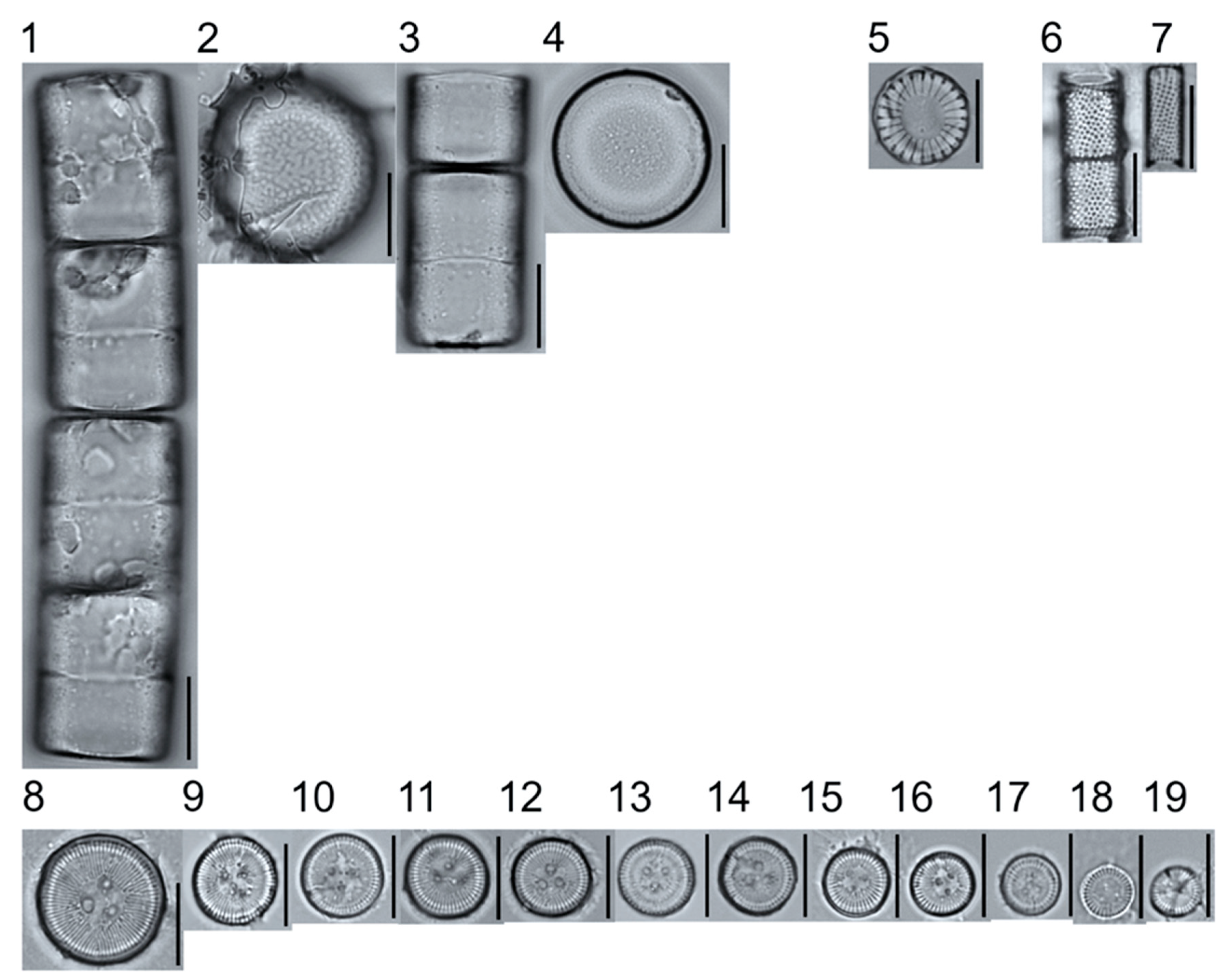
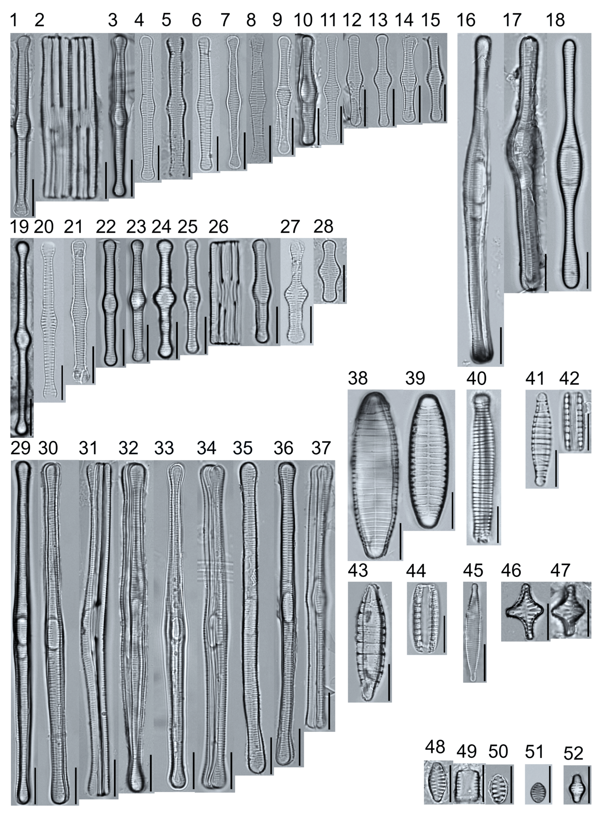
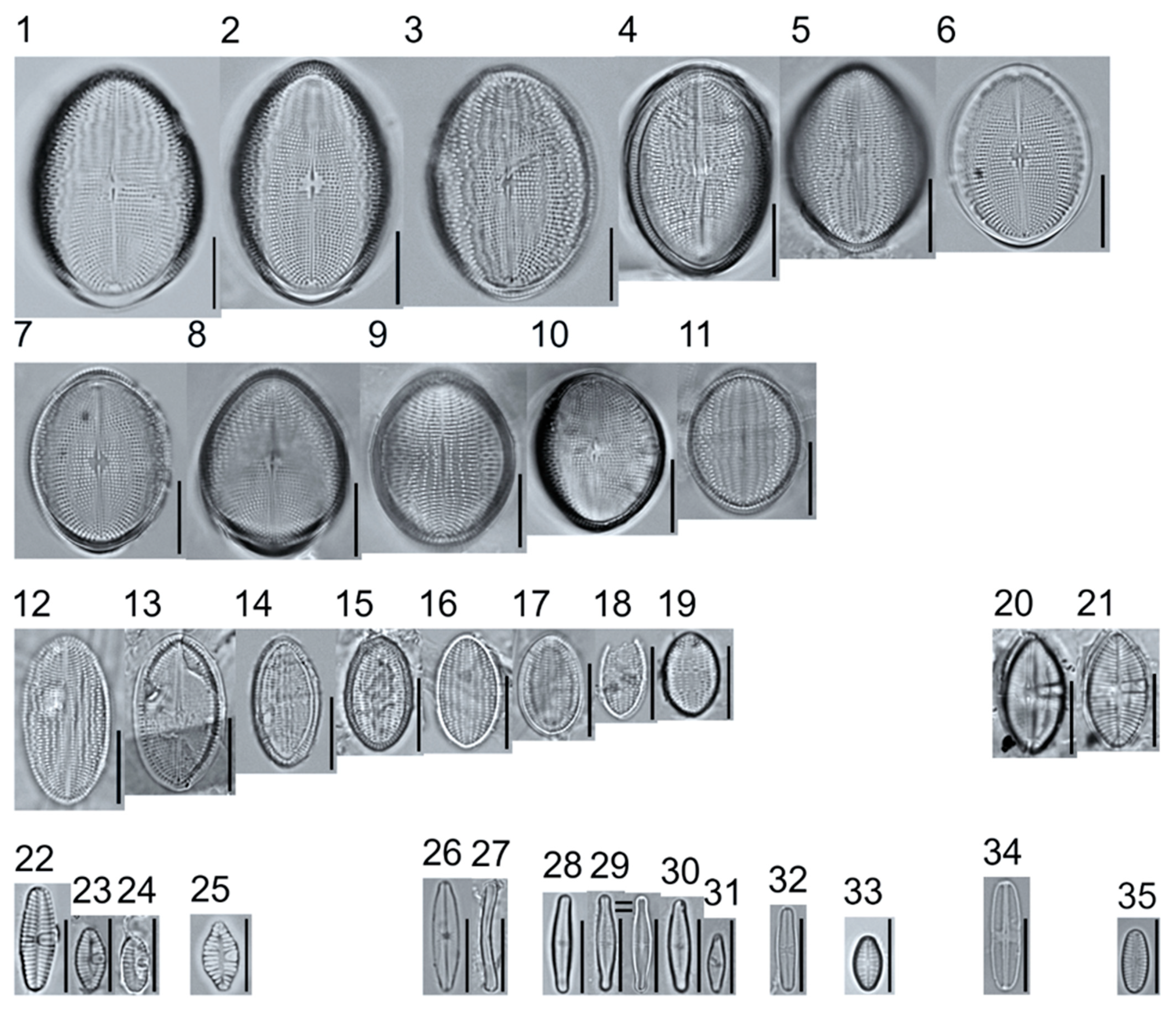
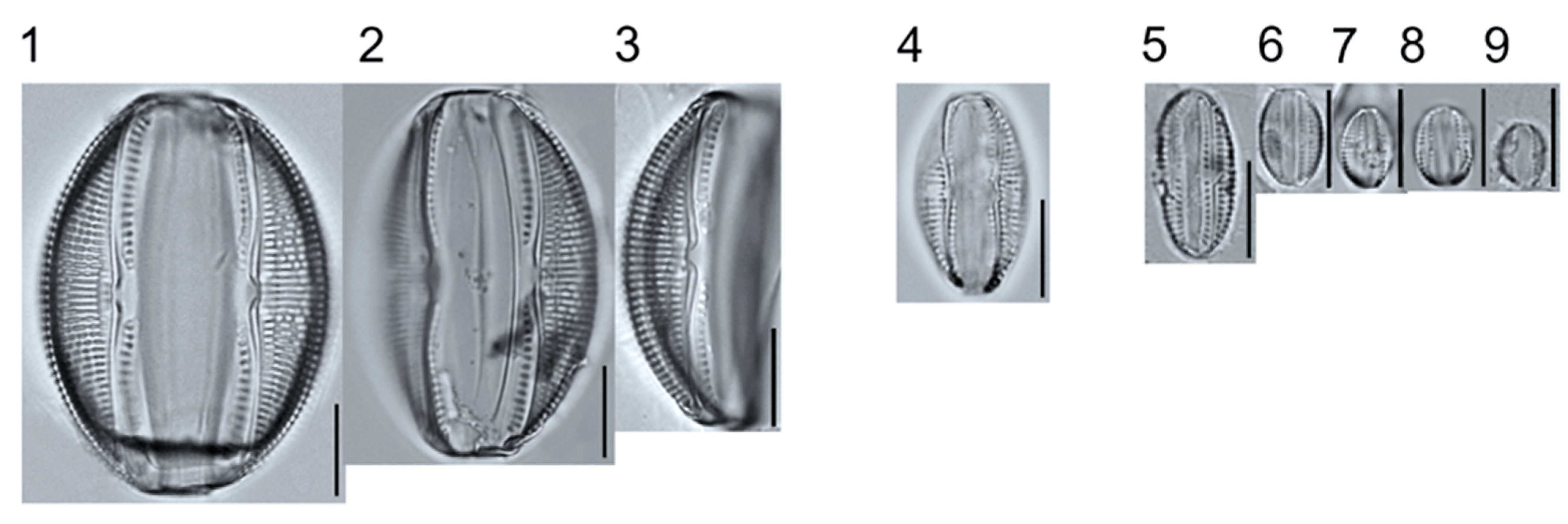
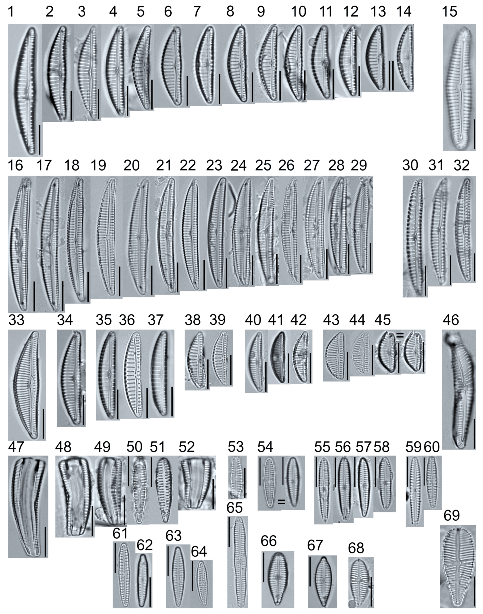
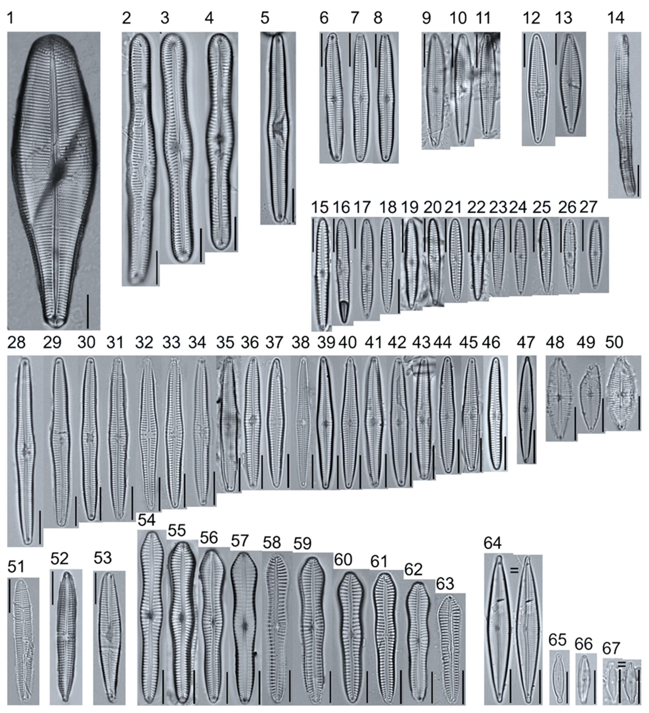
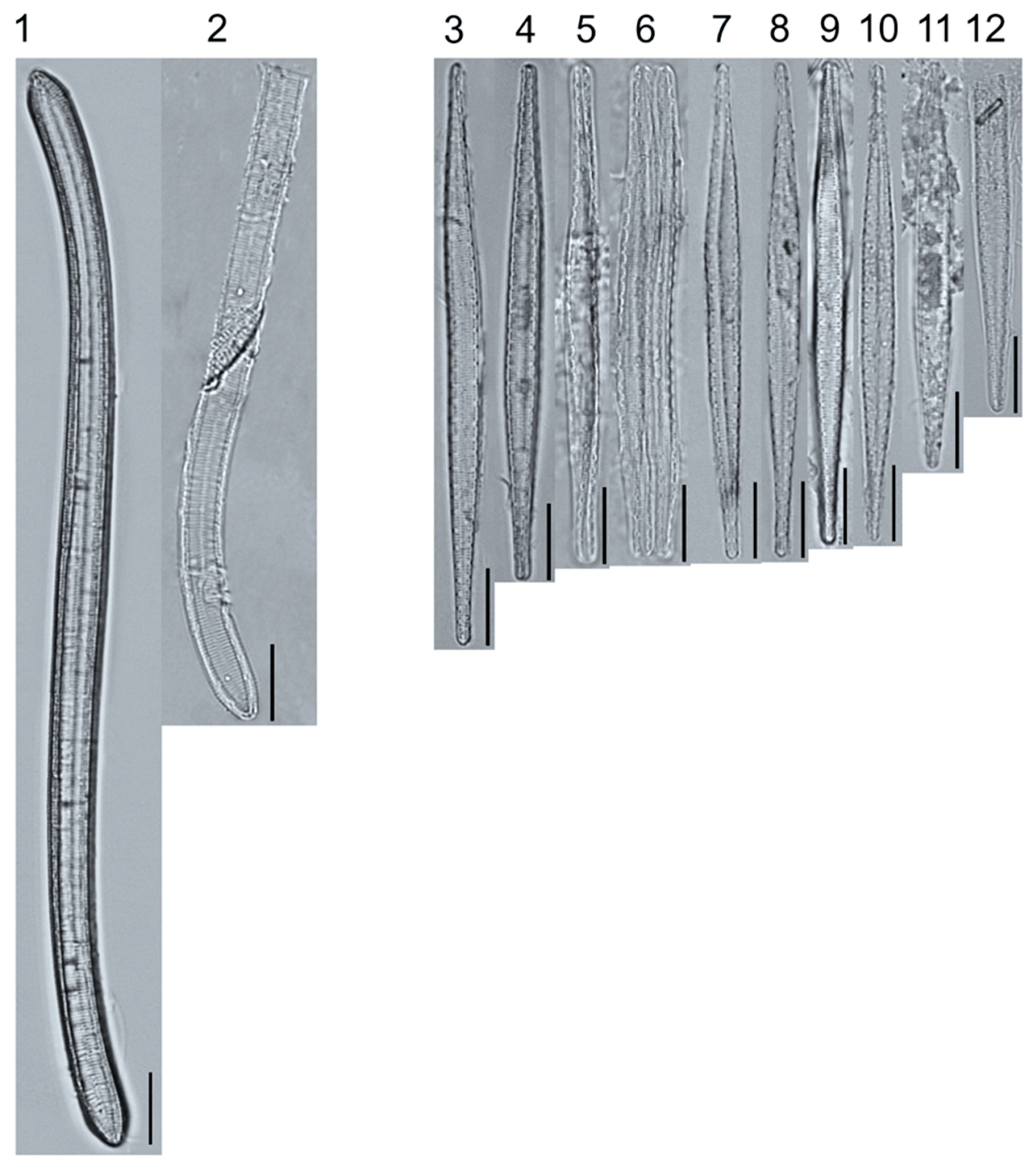
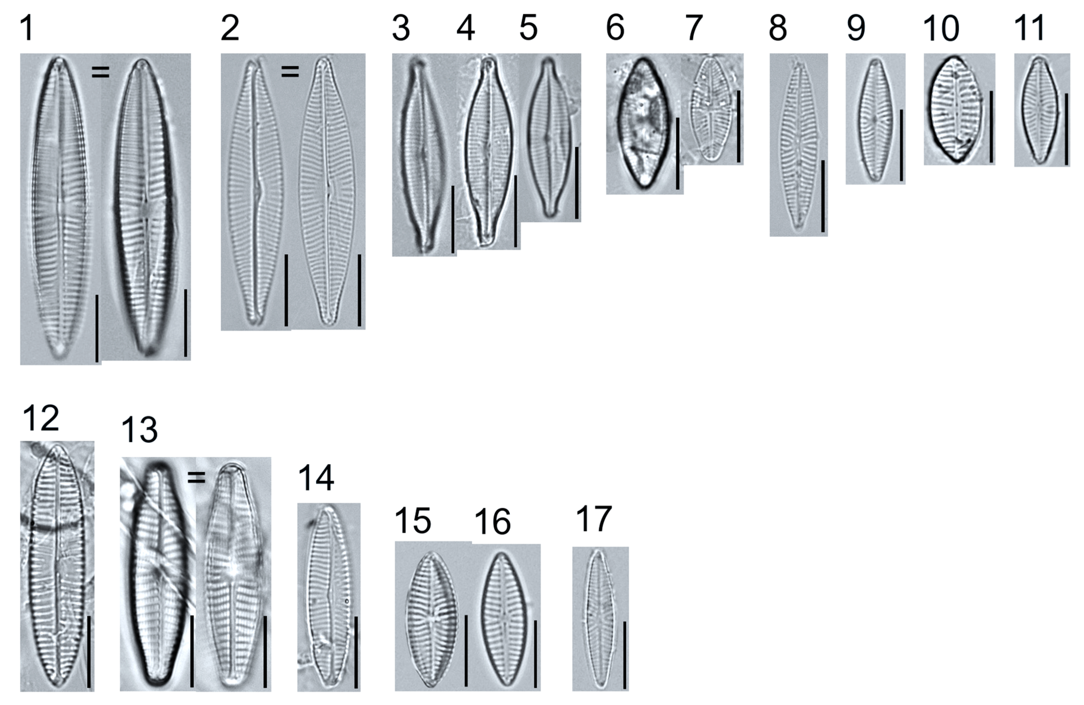
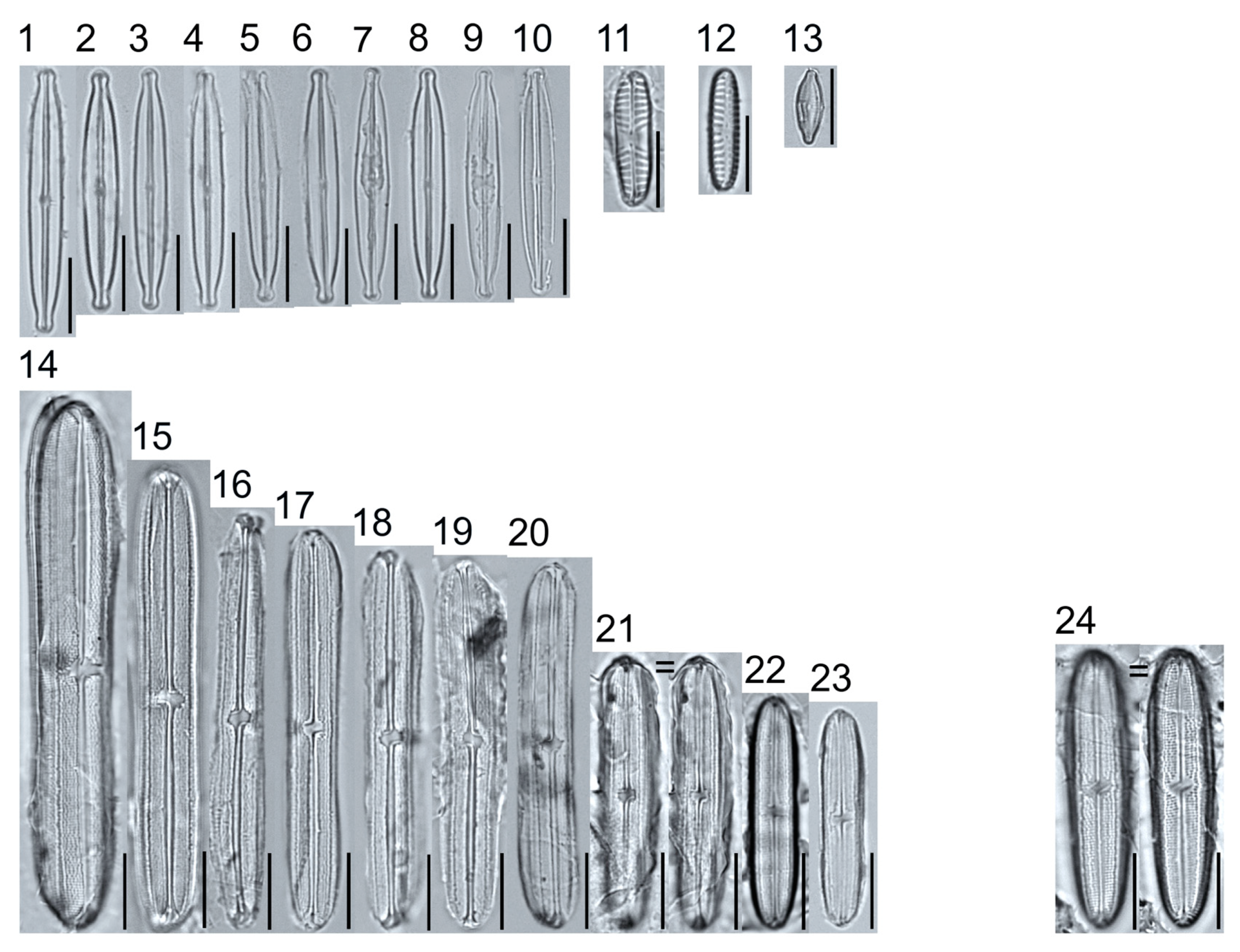
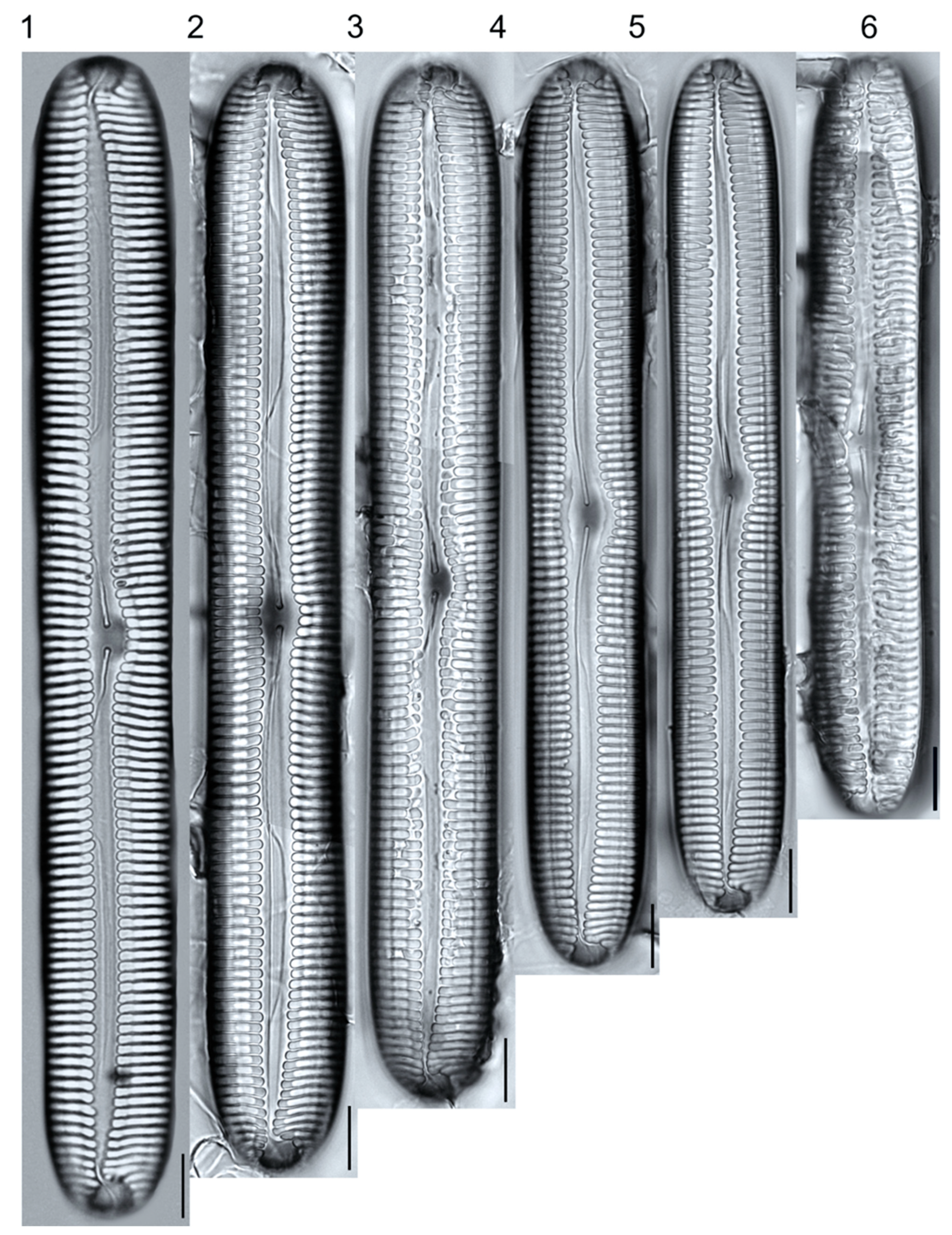
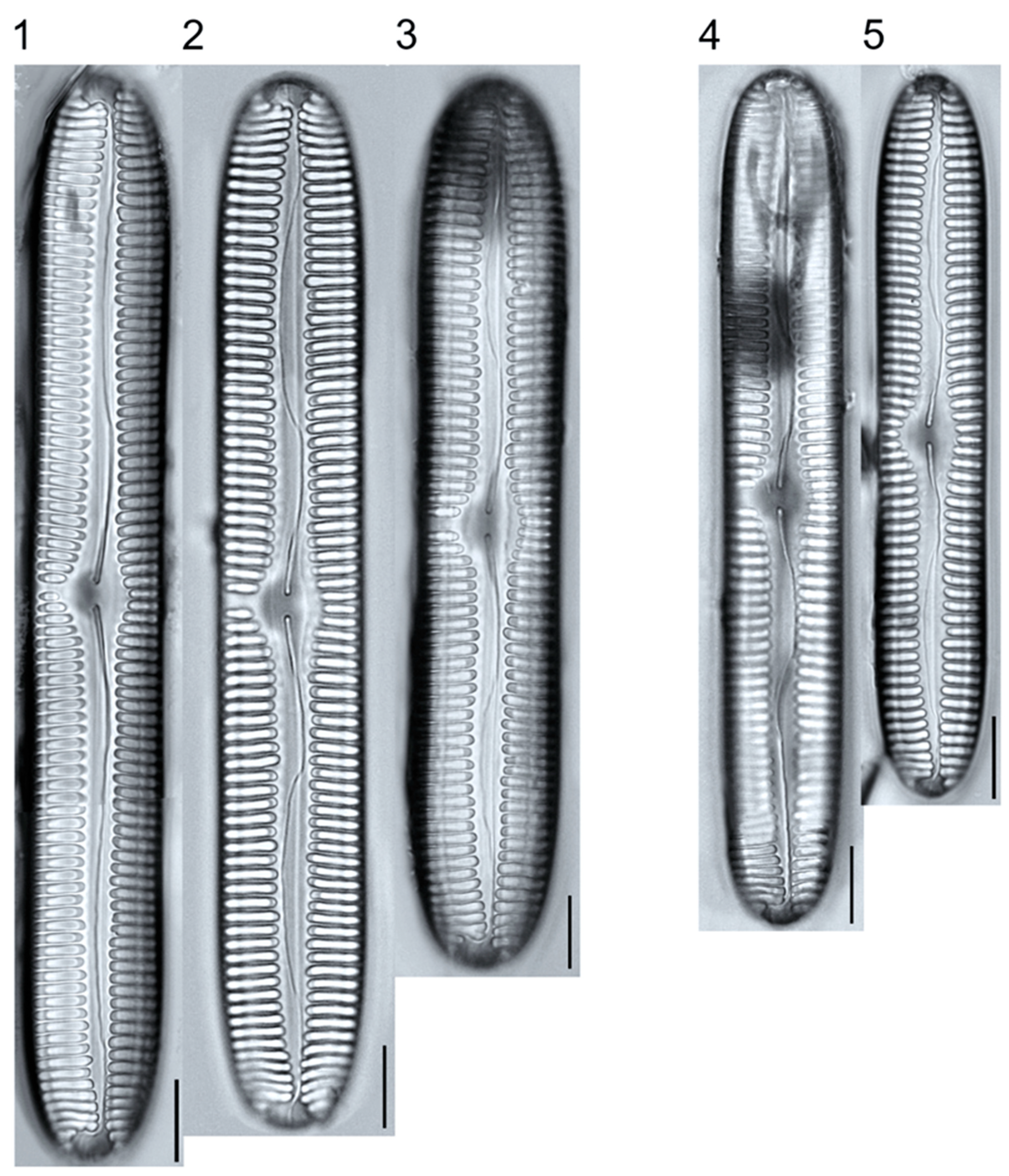
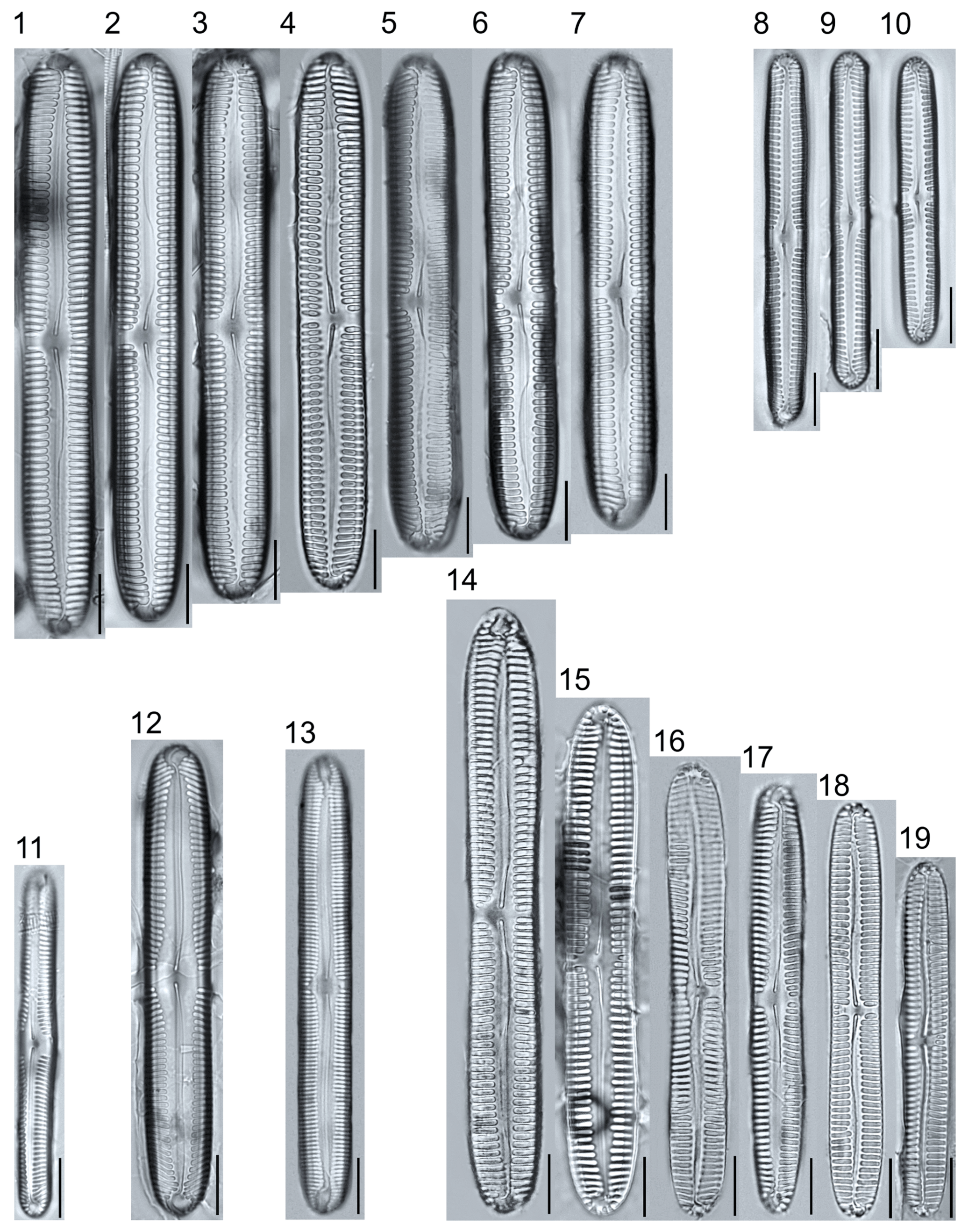
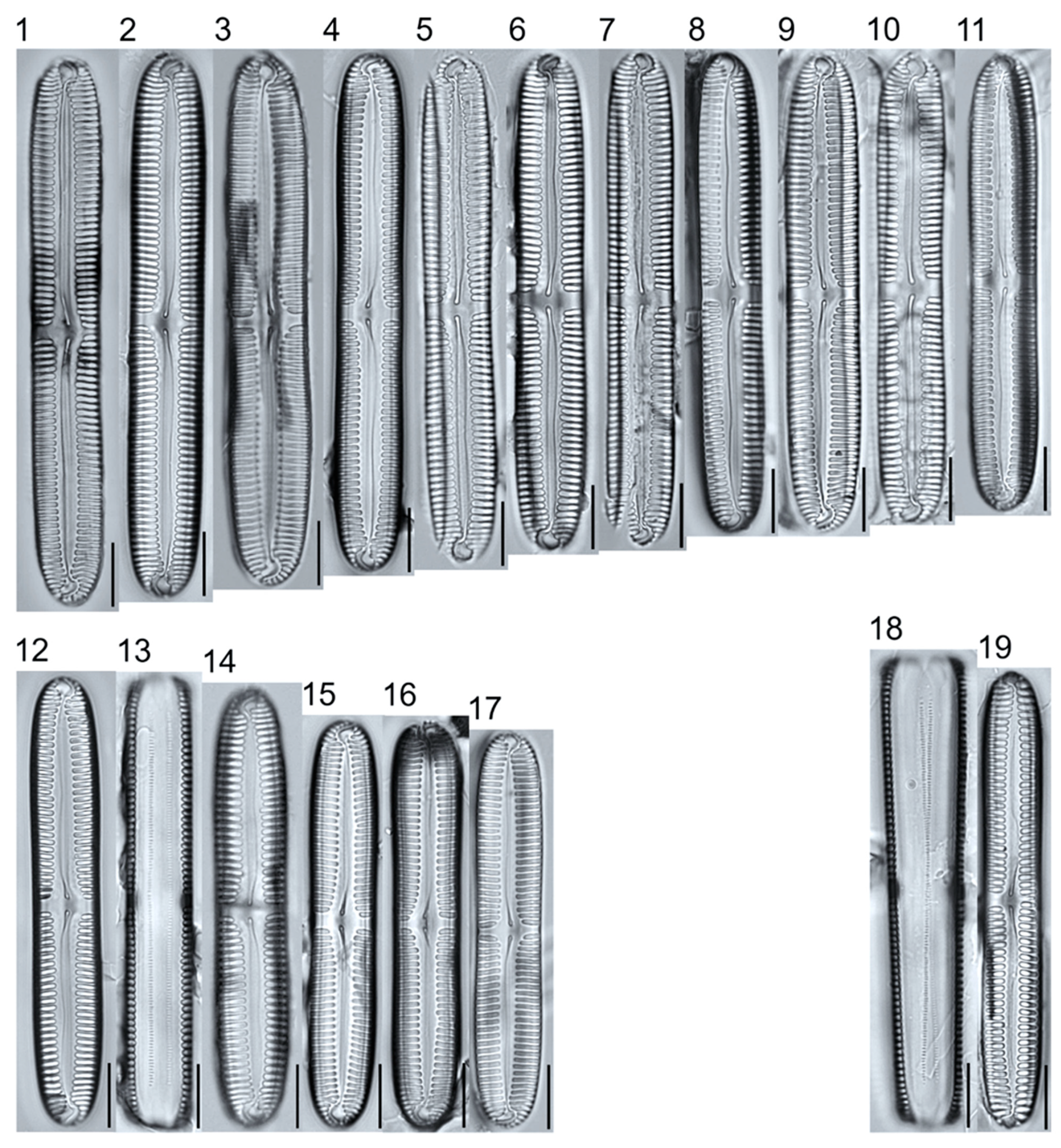
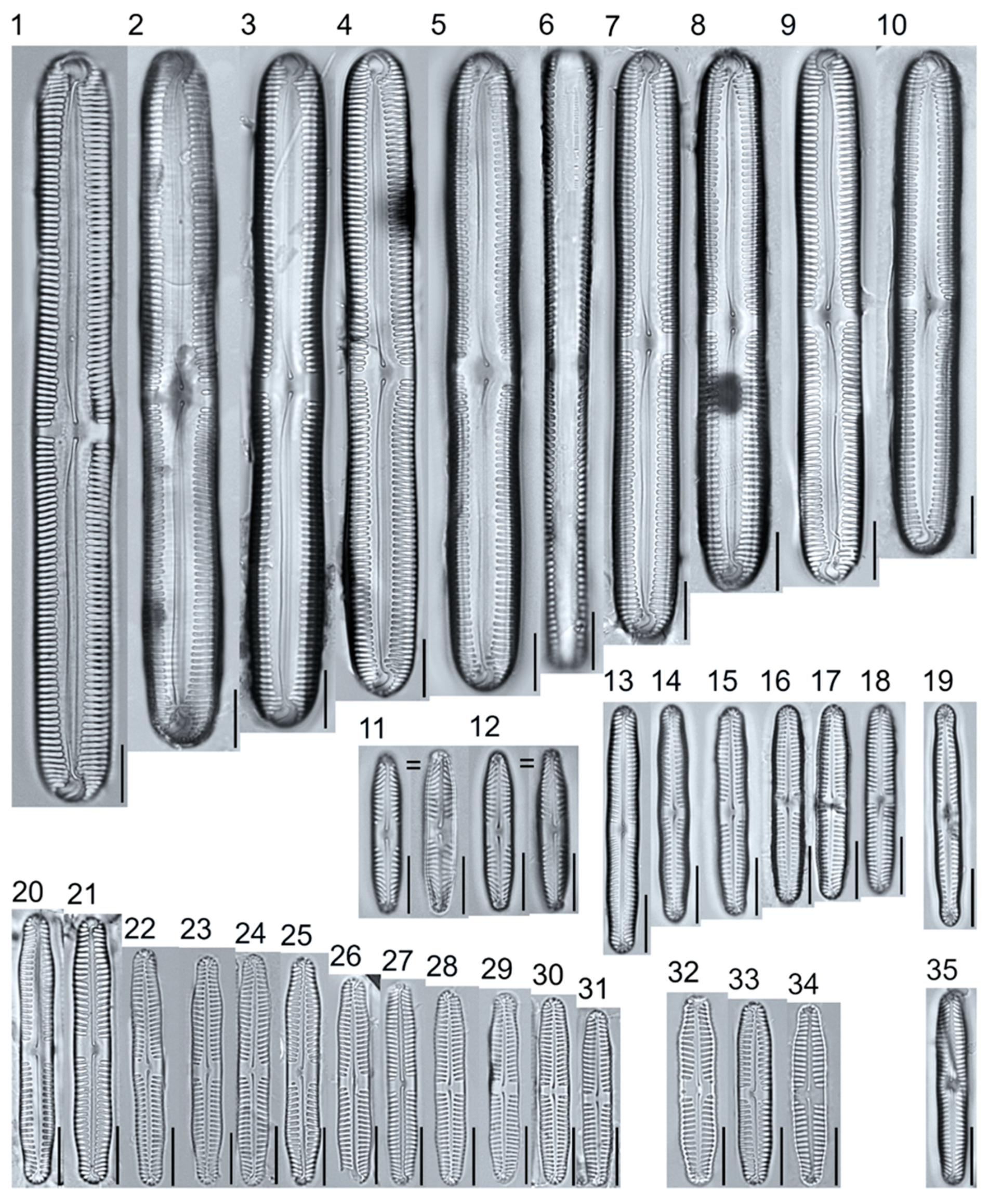
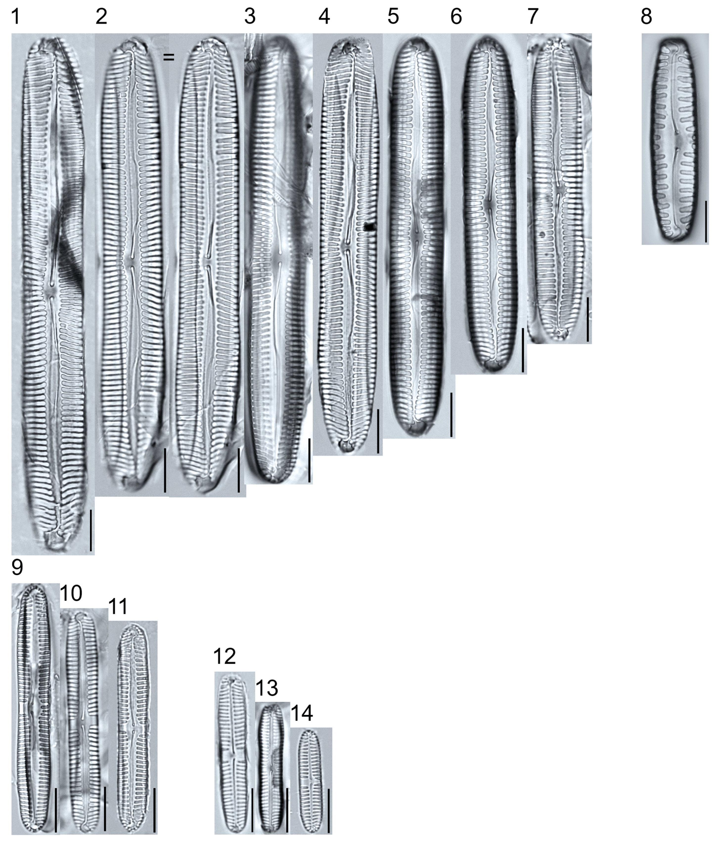
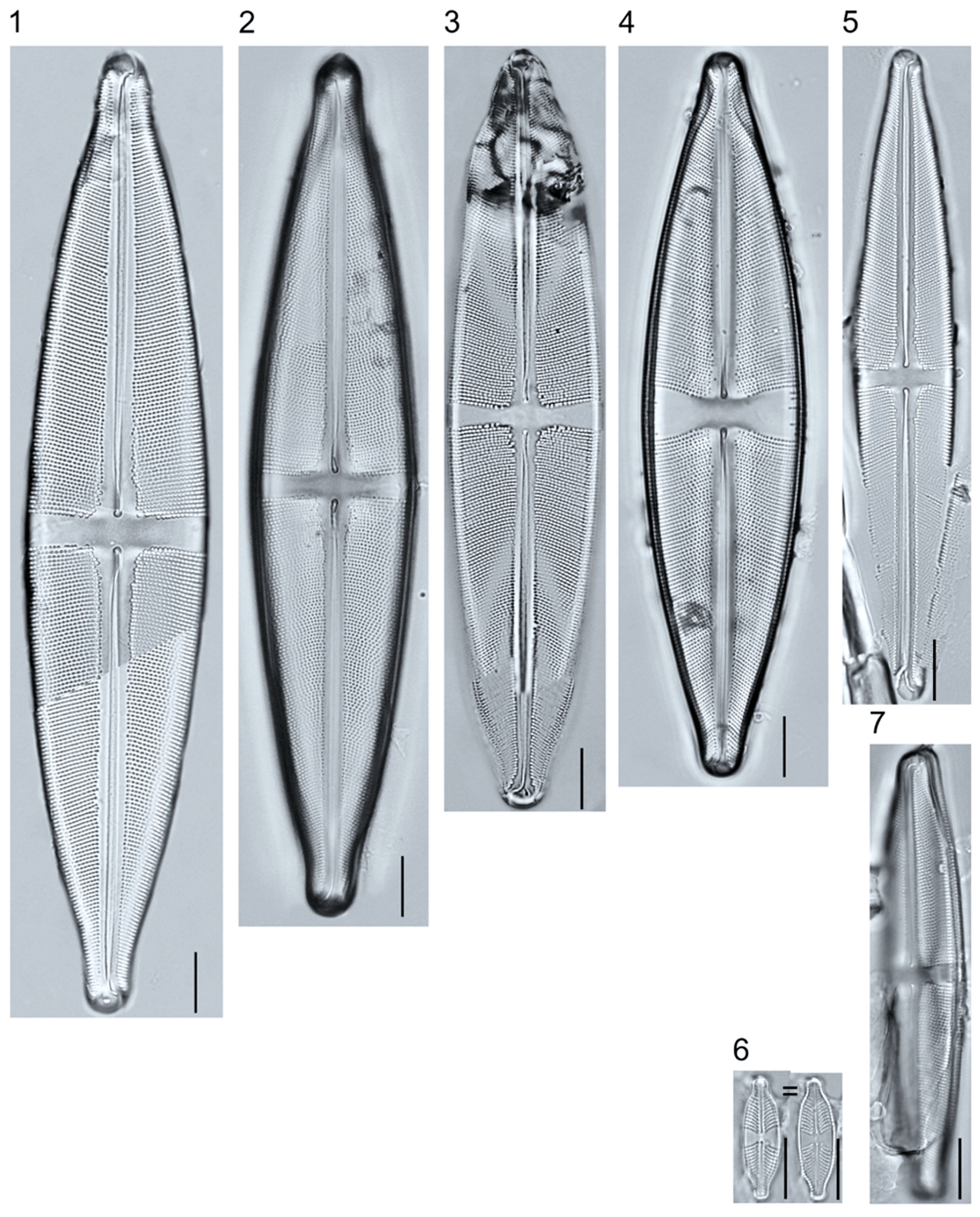
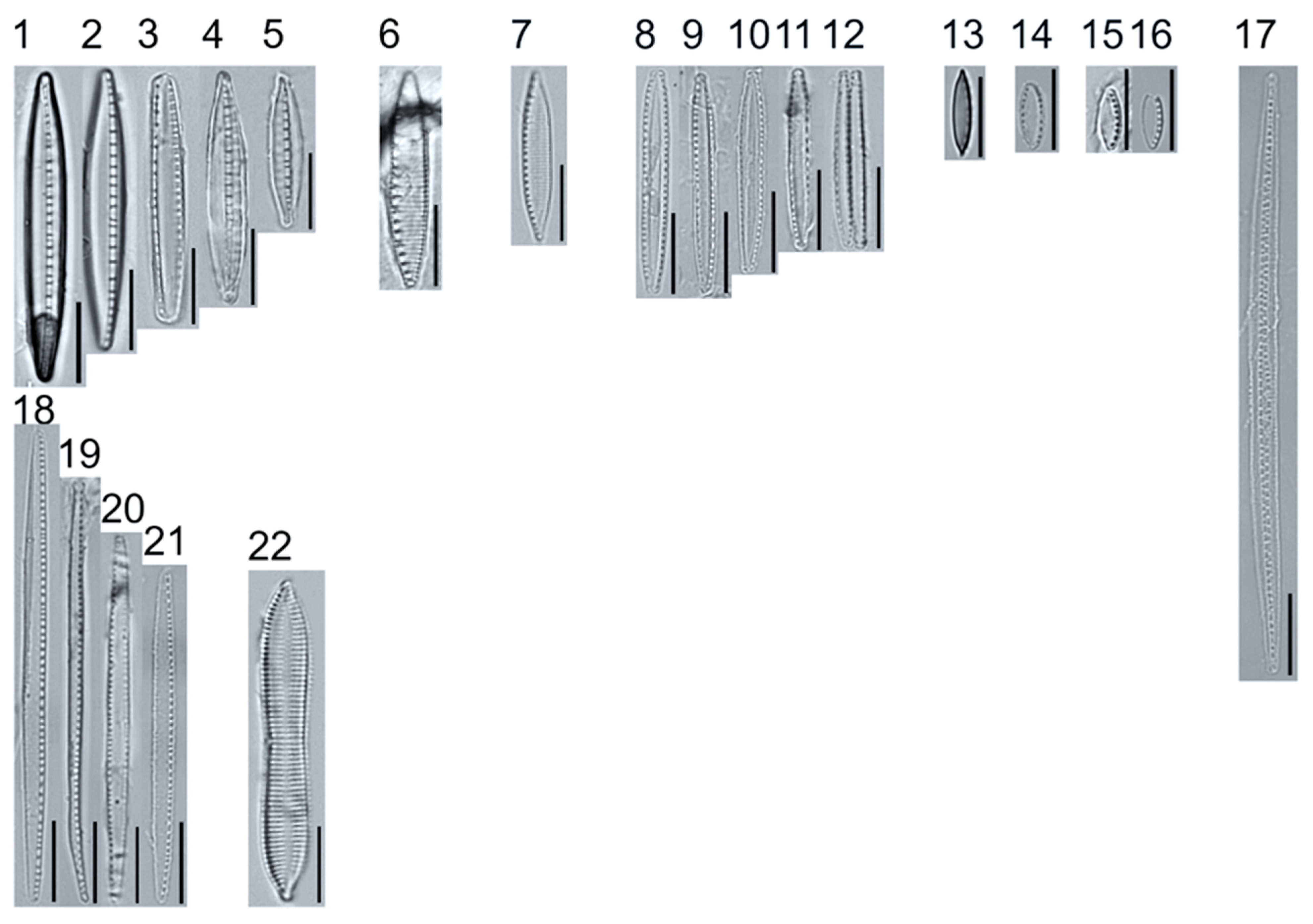
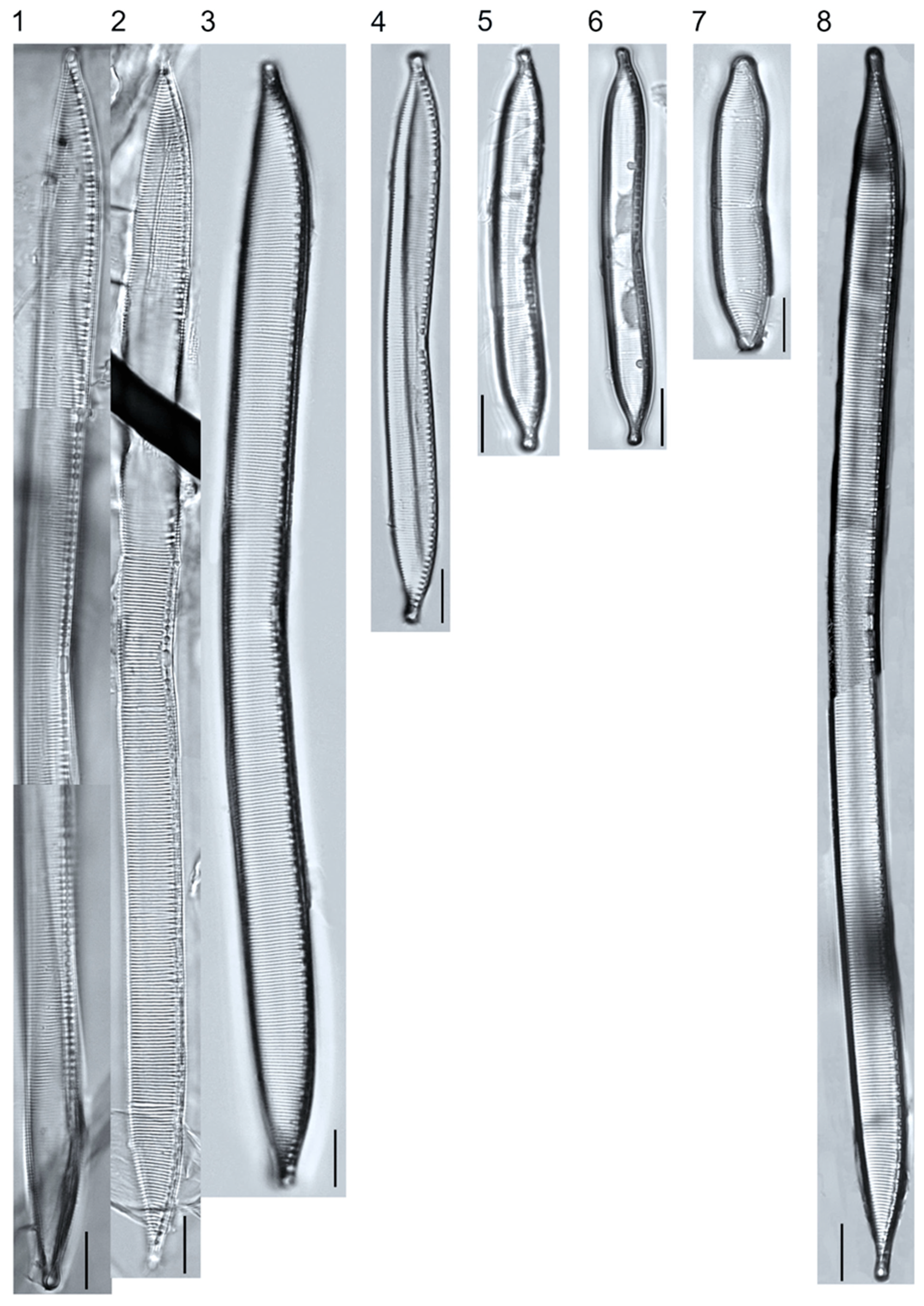
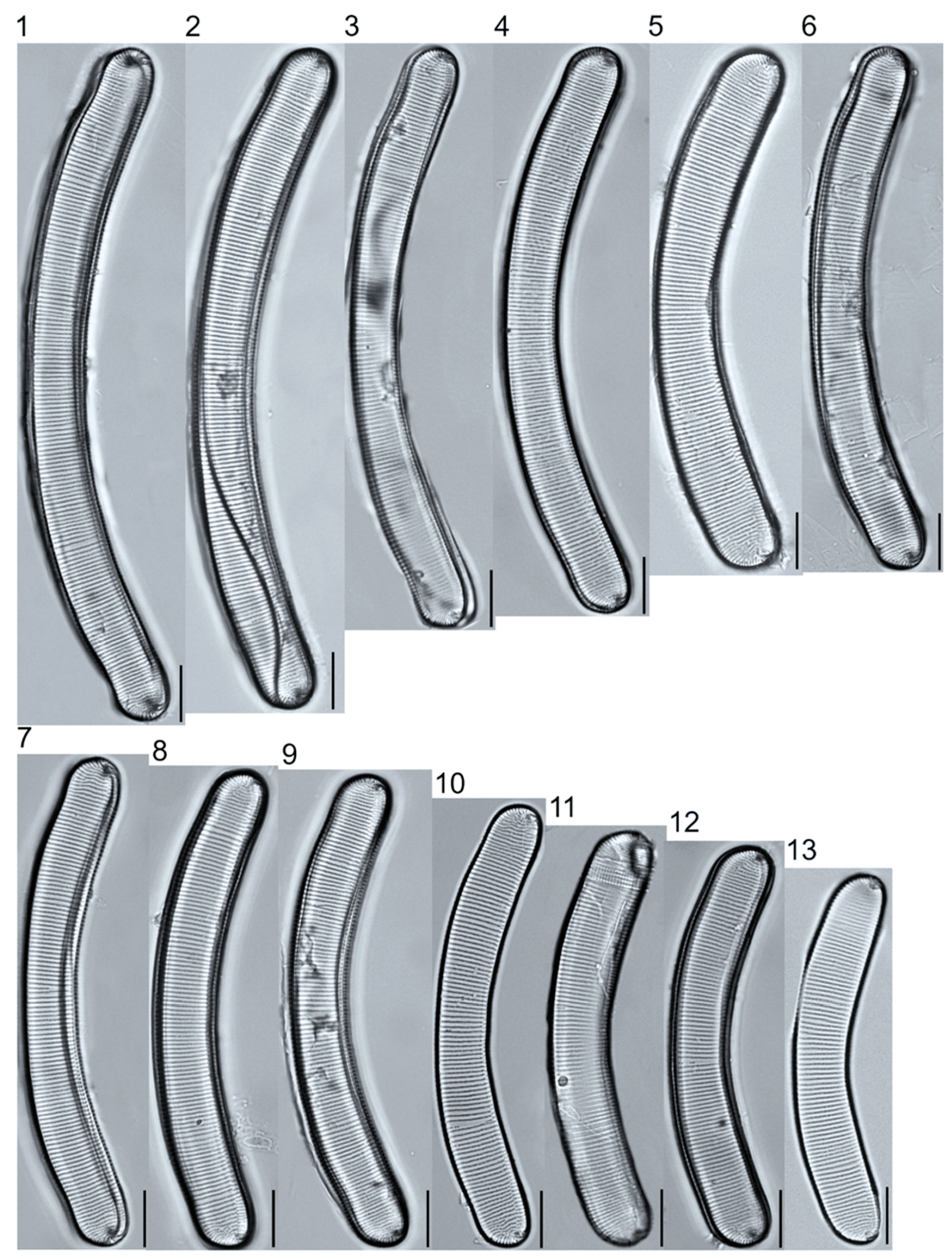
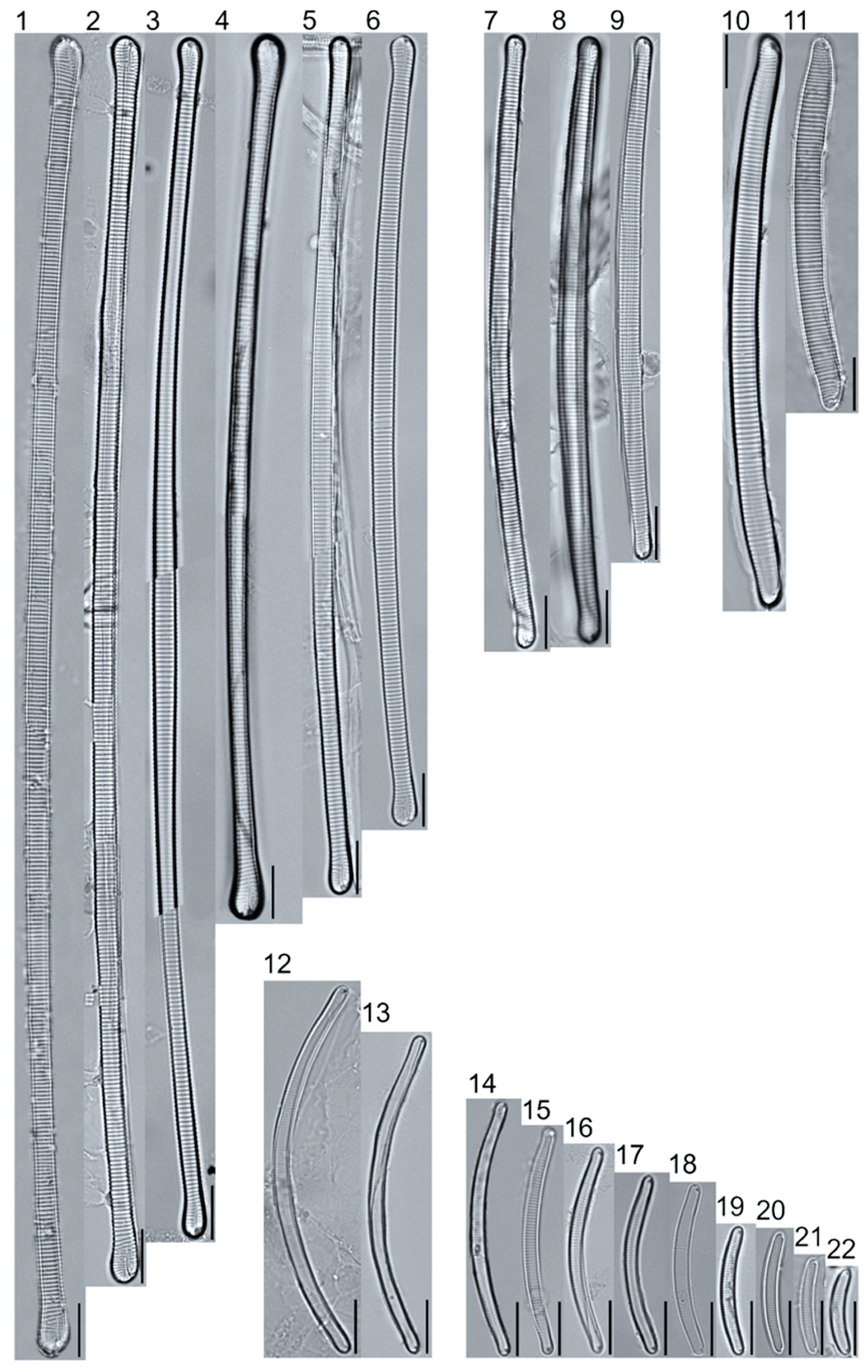
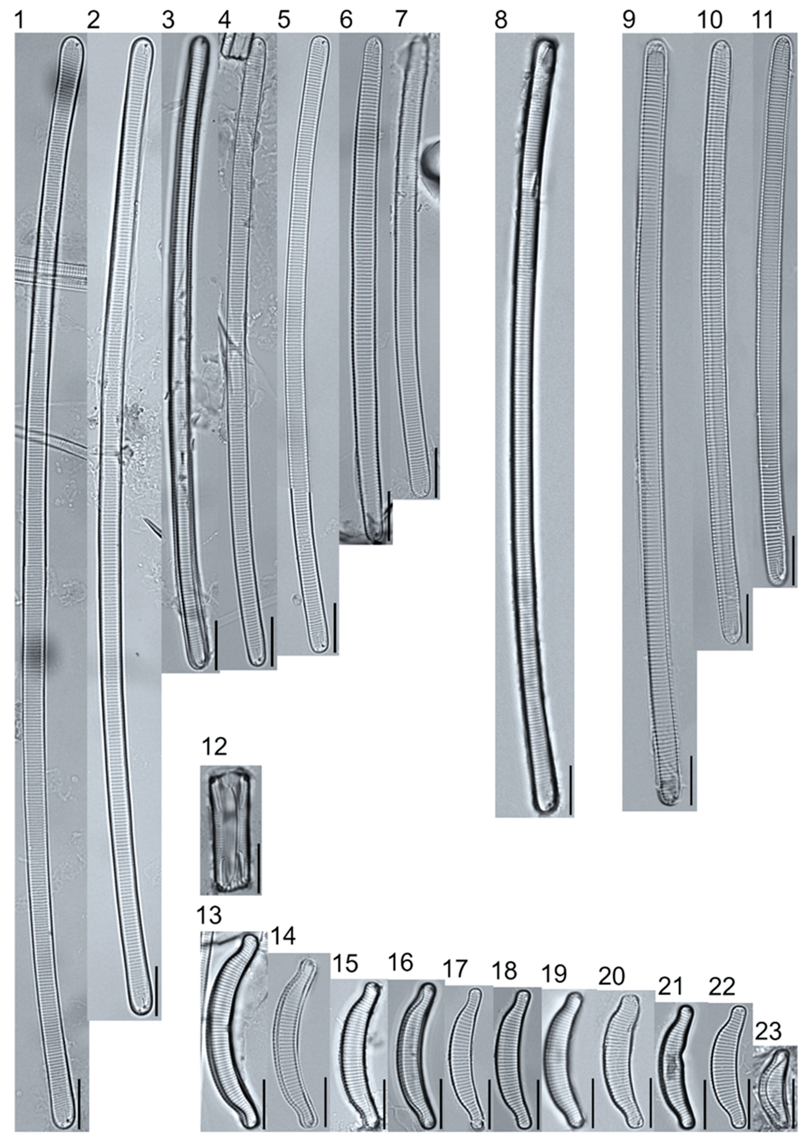
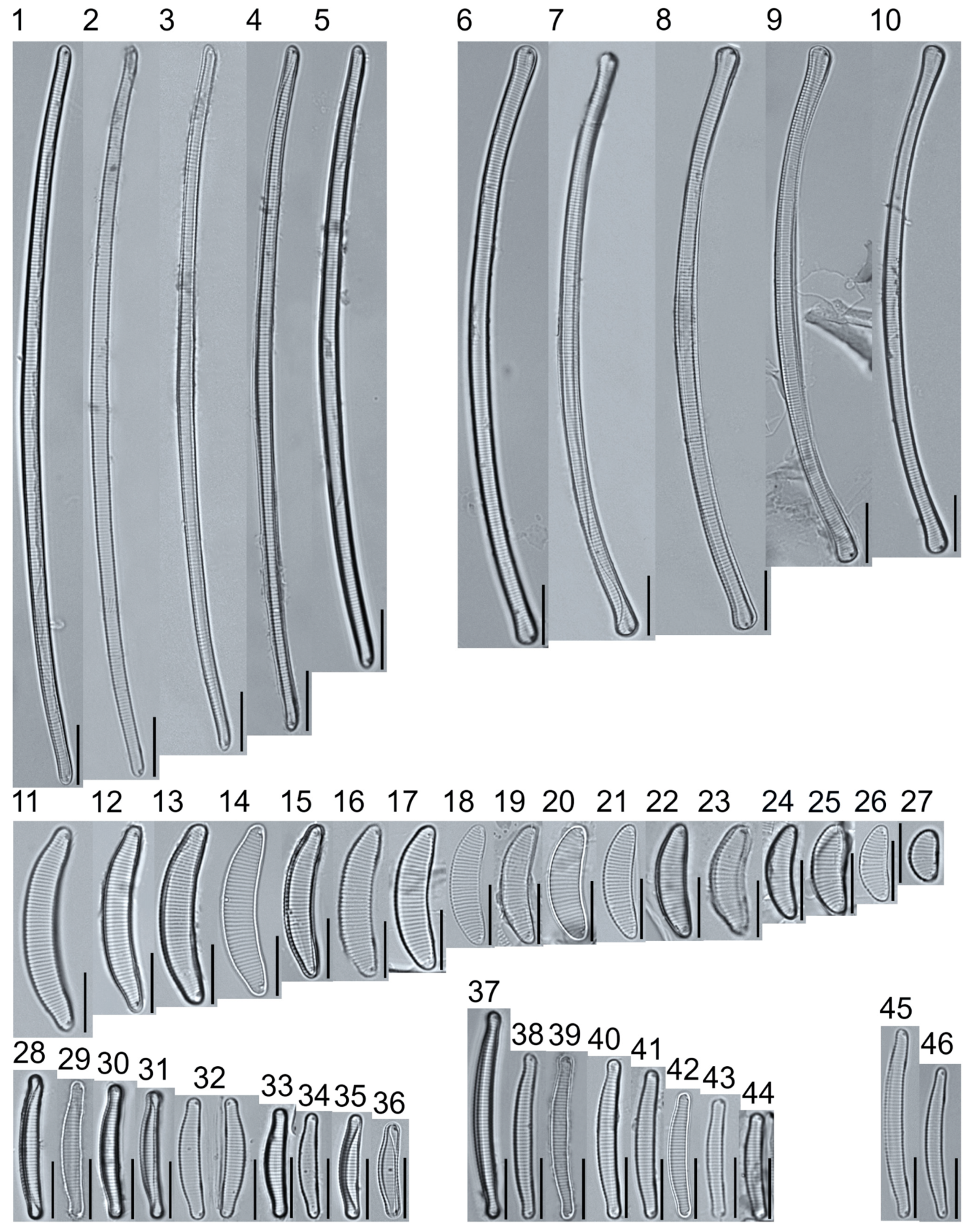
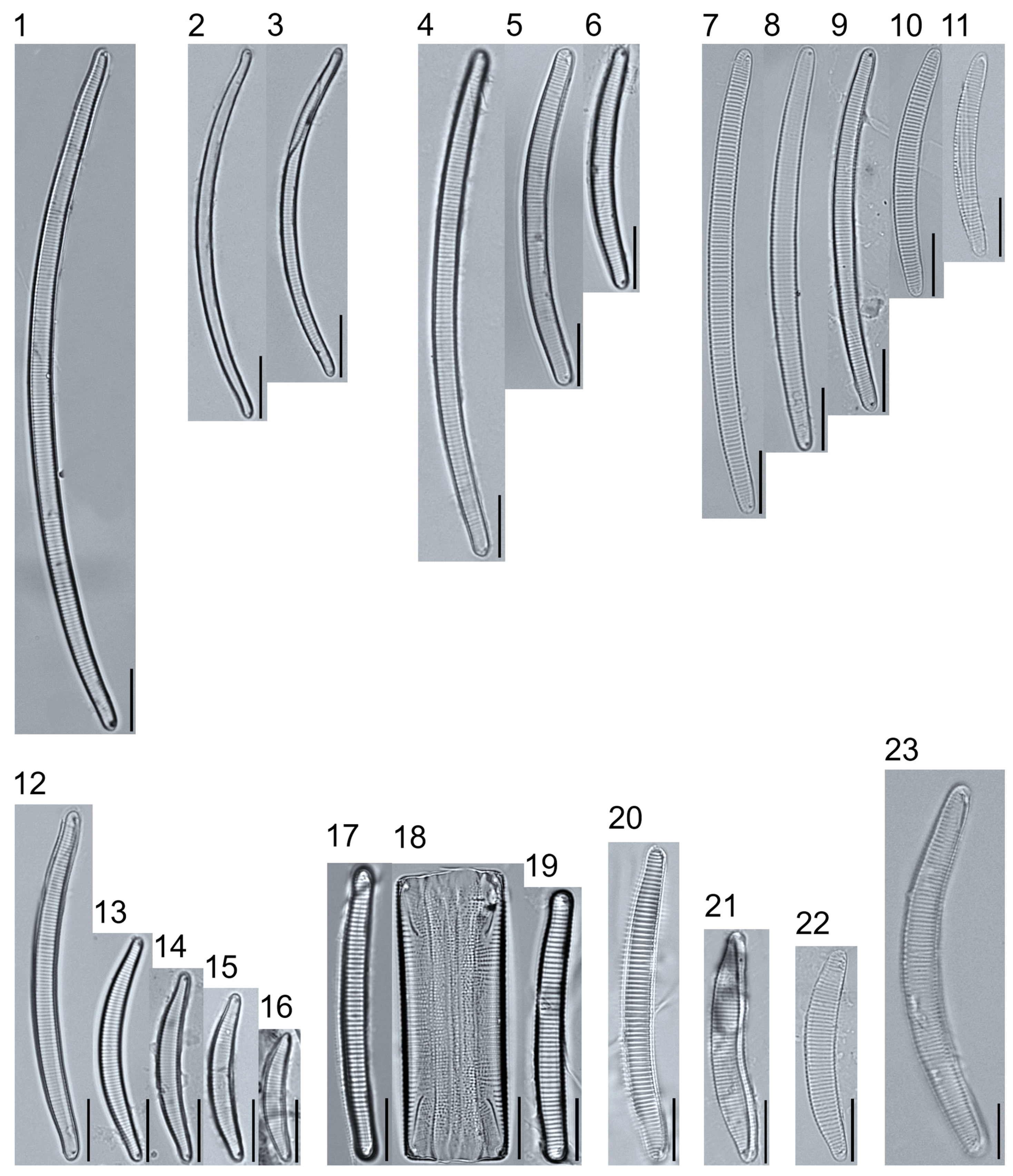
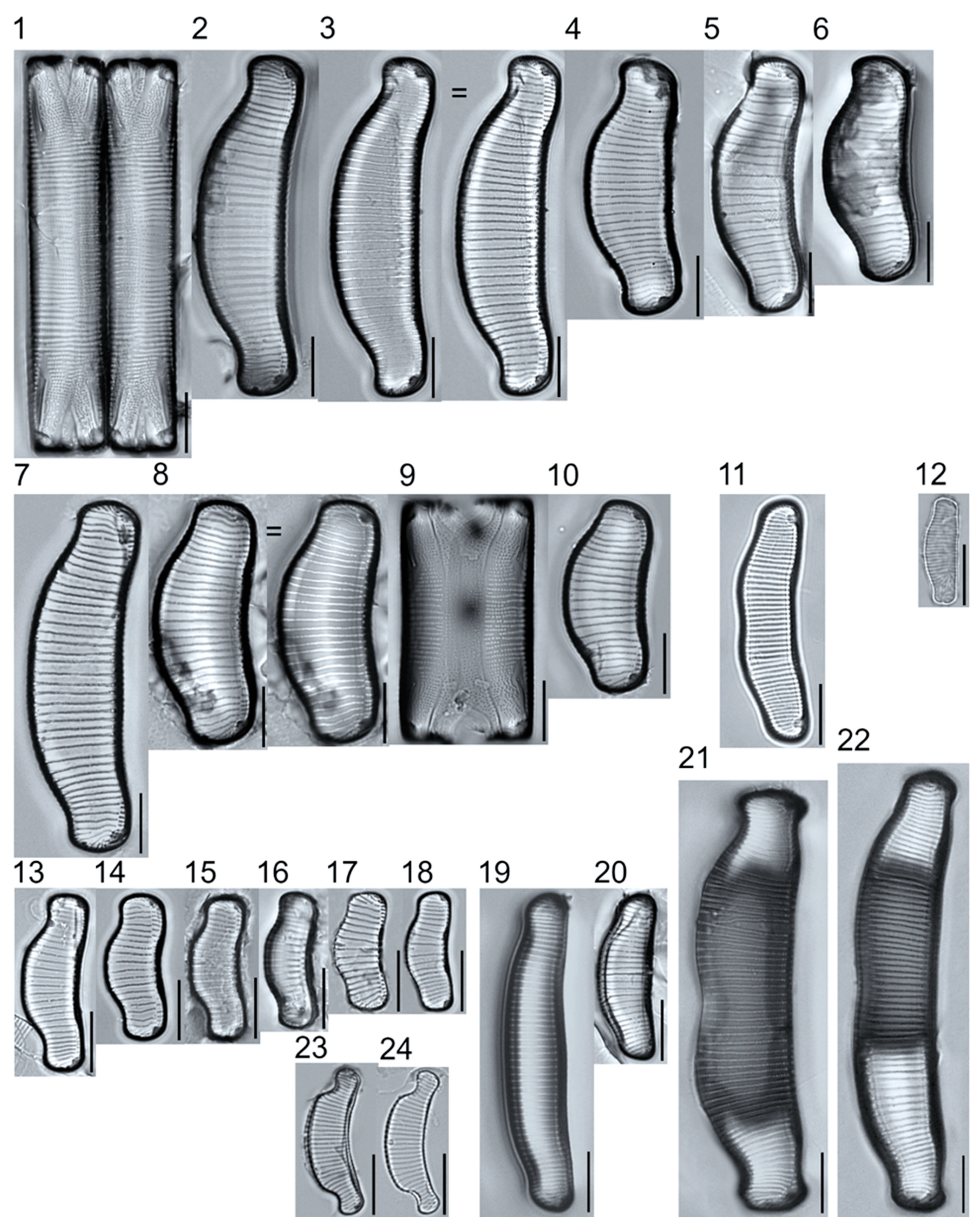
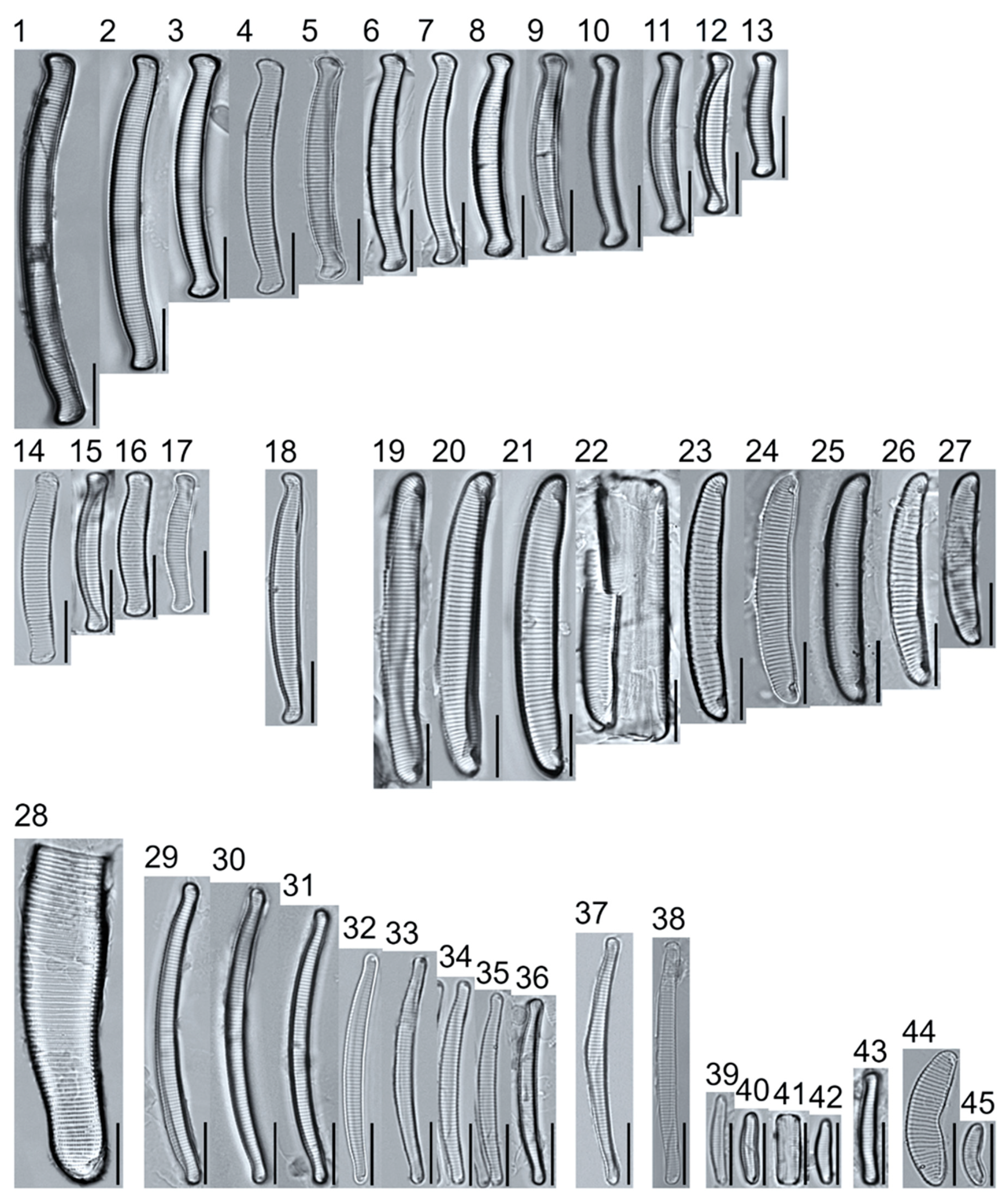
Table 1.
The overall sampling season (5 sampling dates × 4 replicate plots per fen = 20) mean and ±1 standard deviation (SD) for physiochemical characteristics of the rich, moderate, and poor fen sites. Ranges represent the minimum and maximum of measurements taken across the growing season (May–August 2017).
| Rich | Moderate | Poor | |||||||
|---|---|---|---|---|---|---|---|---|---|
| Characteristic | Mean | SD | Range | Mean | SD | Range | Mean | SD | Range |
| Water depth (cm) | 27.5 | 7.95 | 20–35 | 34.0 | 11.4 | 20–46 | 26.6 | 8.86 | 16–34 |
| Water temperature (°C) | 18.5 | 2.29 | 15–21 | 18.0 | 2.88 | 14–21 | 15.2 | 3.53 | 11–20 |
| Water column pH | 6.46 | 1.29 | 5.4–8.9 | 6.42 | 1.32 | 5.3–8.5 | 5.77 | 1.03 | 4.8–7.6 |
| DO (mg L−1) | 3.92 | 1.95 | 2.0–7.0 | 5.71 | 1.49 | 4.3–7.8 | 3.81 | 2.42 | 1.0–7.1 |
| Conductivity (µS) | 39.0 | 5.53 | 31–45 | 25.4 | 2.69 | 24–28 | 40.8 | 5.75 | 34–48 |
| TDN (mg L−1) | 1.51 | 0.19 | 1.3–1.8 | 1.35 | 0.26 | 1.0–1.6 | 1.65 | 0.29 | 1.2–2.0 |
| NO3− (µg L−1) | 7.66 | 2.14 | 6.2–8.9 | 13.2 | 7.39 | 7.2–26.0 | 15.8 | 9.59 | 7.4–27 |
| PO4− (µg L−1) | 8.56 | 3.40 | 6.4–14 | 7.54 | 2.95 | 4.3–10.7 | 20.9 | 6.21 | 15–28 |
| DOC (mg L−1) | 32.6 | 4.32 | 26–37 | 29.7 | 3.14 | 27–35 | 62.4 | 9.41 | 51–77 |
| PAR (µmol cm2 s−1) | 254.4 | 246.6 | 38–448 | 266.1 | 225.1 | 84–672 | 242.3 | 207.0 | 27–484 |
Note: DO = dissolved oxygen, TDN = total dissolved nitrogen, NO3− = nitrate, PO4− = phosphate, DOC = dissolved organic carbon, PAR = photosynthetically active radiation.
Table 2.
List of taxa documented in this study, with authorship, dimension range, voucher image references to plates and figures, fen type, accessioned samples at Ball State University, and taxa status in the Red List developed in Germany [25]: 1 = threatened with extinction; 2 = highly threatened; 3 = threatened; G = threat of unknown extent; R = extremely rare; V = near threatened; D = data deficient; * = not threatened; ♦ = not evaluated.
| Taxon/Author | Dimensions | Plates and Figure | Fen Type | Sample | [25] |
|---|---|---|---|---|---|
| Achnanthidium alpestre (R. L. Lowe and Kociolek) R. L. Lowe and Kociolek in J. R. Johans. et al. 2004 | L: 15.0–15.2, W: 3.8 | Plate 3, Figures 26 and 27 | Poor | 25000 | ♦ |
| Achnanthidium cf. gracillimum (F. Meister) Lange-Bert. 2004 | L: 8.2–13.6, W: 2.5–3.1 | Plate 3, Figures 28–31 | Rich; Poor | 25002 | 2 |
| Achnanthidium minutissimum var. jackii (Rabenh.) Lange-Bert. 1989 | L: 11.7, W: 2.4 | Plate 3, Figure 32 | Poor | 25003a | D |
| Achnanthidium sp. 1 APP | L: 7.6, W:4.1, S: 18–20 | Plate 3, Figure 33 | Poor | 25001 | ♦ |
| Amphora copulata (Kütz.) Schoeman and R. E. M. Archibald 1986 | L: 21.0, W: 5.2, S: 14–15 | Plate 4, Figure 4 | Moderate | 25005a | * |
| Amphora ovalis (Kütz.) Kütz. 1844 | L: 34.3–43.9, W: 8.5–10.8, S: 11–13 | Plate 4, Figures 1–3 | Rich; Moderate | 25006 | * |
| Amphora pediculus (Kütz.) Grunow 1875 | L: 6.5–17.1, W: 1.5–3.7, S: 13–25 | Plate 4, Figures 5–9 | Moderate; Poor | 25007a | * |
| Aulacoseira ambigua (Grunow) Simonsen 1979 | D: 4.7–7.5, MH: 9.2–11.9, A: 18–20 | Plate 1, Figures 6 and 7 | Rich; Poor | 25008 | * |
| Caloneis schroederoides Foged 1981 | L: 23.3–35.8, W: 5.2–6.0, S: 11–15 | Plate 15, Figures 12–14 | Moderate | 25102 | ♦ |
| Cocconeis pediculus Ehrenb. 1838 | L: 20.0–33.2, W: 16.3–23.7, S: 14–20 | Plate 3, Figures 1–11 | Rich; Moderate; Poor | 25009 | * |
| Cocconeis placentula sensu lato Ehrenb. 1838 | L: 11.9–23.2, W: 6.6–12.9, S: 16–25 | Plate 3, Figures 11–19 | Rich; Moderate; Poor | 25010 | * |
| Denticula cf. kuetzingii Grunow 1862 | L: 18.5 S: 16–19 F: 6 | Plate 2, Figure 44 | Rich | 25092b | ♦ |
| Diadesmis sp. 1 APP | L: 14.7–18.5, W: 5.9–7.4, S: 18–22 | Plate 8, Figures 6 and 7 | Moderate | 25087b | ♦ |
| Diatoma ehrenbergii Kütz. 1844 | L: 40.9, W: 6.1, C: 11–13 | Plate 2, Figure 40 | Poor | 25004b | * |
| Diatoma moniliformis (Kütz.) D.M.Williams 2012 | L: 16.2–25.7, W: 5.5, C: 6–8 | Plate 2, Figures 41 and 42 | Rich; Poor | 25012 | * |
| Diatoma vulgaris Bory 1824 | L: 36.8–45.6, W: 11.2–12.8, C: 7–9 | Plate 2, Figures 38 and 39 | Moderate | 25013a | * |
| Encyonema groenlandica (Foged) Kulikovskiy and Lange-Bert. 2009 | L: 28.6–29.6, W: 5.4–5.8, S: 6–8 | Plate 5, Figures 34 and 36 | Rich; Moderate | 25014a | ♦ |
| Encyonema cf. groenlandica (Foged) Kulikovskiy and Lange-Bert. 2009 | L: 18.2–19.3, W: 4.9–5.2, S: 10–12 | Plate 5, Figures 38 and 39 | Rich; Moderate | 25015a | ♦ |
| Encyonema lunatum var. alaskaense (Foged) Metzeltin and Lange-Bert. 2009 | L: 36.8–39.7, W: 4.8–5.0, S: 8–10 | Plate 5, Figures 30–32 | Rich; Moderate | 25016a | ♦ |
| Encyonema montana Bahls 2017 | L: 14.1–17.3, W: 5.5–7.0, S: 12–14 | Plate 5, Figures 43–45 | Rich; Poor | 25017a | ♦ |
| Encyonema neogracile Krammer 1997 | L: 31.5–44.7, W: 4.7–6.3, S: 11–15 | Plate 5, Figures 16–29 | Rich; Moderate; Poor | 25018a | 3 |
| Encyonema paucistriatum (A. Cleve) D. G. Mann 1990 | L: 22.1–42.8, W: 5.4–6.5, S: 8–11 dorsal, 12–13 ventral | Plate 5, Figures 1–14 | Rich; Moderate; Poor | 25019a | 2 |
| Encyonema procerum Krammer 1997 | L: 31.4, W: 6.8, S: 10–12 | Plate 5, Figure 34 | Moderate | 25015b | 1 |
| Encyonema schimanskii Krammer 1997 | L: 17.4–20.0, W: 4.5–5.0, S: 14–15 | Plate 5, Figures 40–42 | Rich; Moderate | 25016b | G |
| Encyonema silesiacum (Bleisch in Rabenh.) D. G. Mann 1990 | L: 36.4, W: 8.8, S: 11–12 | Plate 5, Figure 33 | Moderate | 25007b | * |
| Encyonopsis cf. microcephala (Grunow) Krammer 1997 | L: 15.9, W: 3.7, S: 19–20 | Plate 6, Figure 65 | Rich | 25021a | * |
| Encyonopsis cf. minuta Krammer and E. Reichardt 1997 | L: 12.3, W: 3.4 | Plate 6, Figure 67 | Poor | 25003b | D |
| Encyonopsis montana Bahls 2013 | L: 43.6, W: 7.1, S: 19–20 | Plate 6, Figure 64 | Poor | 25020 | ♦ |
| Encyonopsis thumensis Krammer 1997 | L: 14.7, W: 3.1, S: 20–22 * | Plate 6, Figure 66 | Poor | 25004c | G |
| Eunotia ambivalens Lange-Bert. and Tagliaventi 2011 | L: 110.8–154.1, W: 4.8–5.1, S: 12–14c; 15–16a | Plate 21, Figures 6–10 | Rich | 25022a | G |
| Eunotia arcus Ehrenberg 1837 | L: 27.5–52.9, W: 9.4–10.8, S: 10–12 | Plate 24, Figures 19–20 | Rich | 25023 | V |
| Eunotia cf. bertrandii Lange-Bert. and Tagliaventi 2011 | L: 15.8–25.6, W: 2.9–3.8, S: 17–20 | Plate 22, Figures 28–36 | Rich; Moderate; Poor | 25056 | G |
| Eunotia bidens Ehrenberg 1843 | L: 76.6, W: 13.9, S: 9–10c, 13–14a | Plate 24, Figure 22 | Rich | 25024 | G |
| Eunotia bilunaris (Ehrenb.) Schaarschm. 1881 | L: 35.0–74.1, W: 3.6–4.3, S: 16–19 | Plate 23, Figures 7–11 | Rich; Moderate | 25025 | * |
| Eunotia curtagrunowii Nörpel Schempp and Lange-Bert. 1996 | L: 20.0–29.6, W: 7.0–9.8, S: 8–12 | Plate 24, Figures 13–18 | Rich; Moderate | 25026a | G |
| Eunotia dorofeyukae Lange-Bertalot and Kulikovskiy 2010 | L: 40.7, W: 9.4, S: 11–14 | Plate 24, Figure 11 | Rich | 25048 | R |
| Eunotia ferefalcata Kulikovskiy and Lange-Bert. 2011 | L: 20.7–55.7 *, W: 3.6–4.3 *, S: 17–21* | Plate 23, Figures 12–16 | Rich; Moderate; Poor | 25027 | ♦ |
| Eunotia flexuosa (Brébisson ex Kutz.) Kütz. 1849 | L: 147.6–246.7, W: 3.8–4.5, S: 10–13c; 13–15a | Plate 20, Figures 1–6 | Moderate; Poor | 25028a | 2 |
| Eunotia cf. glacialispinosa Lange-Bert. and Cantonati 2010 | L: 43.9–46.9, W: 4.5–4.6, S: 12–14 | Plate 23, Figures 17–19 | Rich | 25034a | G |
| Eunotia cf. groenlandica (Grunow) Norpel-Schempp and Lange-Bert. nom inval. 1996 | L: 50.2, W: 5.2, S: 11–12 | Plate 23, Figure 20 | Moderate | 25029 | G |
| Eunotia cf. intermedia (Krasske ex Hust.) Nörpel and Lange-Bert. 1993 | L: 39.1, W: 3.1, S: 18–19 | Plate 25, Figure 38 | Moderate | 25019b | 2 |
| Eunotia juettnerae Lange-Bert. 2011 | L: 108.6, W: 4.0, S: 15–17 | Plate 23, Figure 1 | Poor | 25031 | G |
| Eunotia cf. julma Lange-Bert. 2011 | L: 155.8, W: 4.5, S: 15–16 | Plate 21, Figure 8 | Poor | 25032 | ♦ |
| Eunotia julma Lange-Bert. 2011 | L: 93.0–219.2, W: 3.8–5.0, S: 13–18 | Plate 21, Figures 1–7 | Moderate; Poor | 25033 | ♦ |
| Eunotia krammeri Kulikovskiy, Lange-Bertalot, Genkal, and Witkowski 2010 | L: 52.5–58.8, W: 2.4–2.5, S: 18–20 | Plate 23, Figures 2–3 | Poor | 25031 | ♦ |
| Eunotia cf. major (W. Smith) Rabenh. 1864 | L: ~55.1, W: 13.5, S: 11–15 | Plate 25, Figure 28 | Moderate | 25035 | 2 |
| Eunotia cf. mucophila (Lange-Bert., Nörpel-Schempp, and Alles) Lange-Bert. 2007 | L: 59.3–68.5, W: 3.2–3.2, S: 21–23 | Plate 20, Figures 12 and 13 | Poor | 25036a | G |
| Eunotia mucophila (Lange-Bert., Nörpel-Schempp, and Alles) Lange-Bert. 2007 | L: 16.1–47.1, W: 2.7–3.1, S: 18–22 | Plate 20, Figures 14–22 | Poor | 25037a | G |
| Eunotia naegelii Mig. 1907 | L: 103.8–123.1, W: 2.7–3.1, S: 15–17c; 17–20a | Plate 22, Figures 1–5 | Poor | 25038 | 3 |
| Eunotia neocompacta Mayama 1998 | L: 20.4–60.1, W: 3.8–5.2, S: 17–18 | Plate 25, Figures 1–13 | Moderate; Poor | 25039 | 2 |
| Eunotia neocompacta var. vixcompacta Lange-Bert. 2011 | L: 22.6–30.8, W: 3.9–4.7, S: 17–18 | Plate 25, Figures 14–17 | Moderate; Poor | 25040a | G |
| Eunotia paludosa Grunow 1862 | L: 30.1–48.9, W: 3.0–3.5, S: 18–20 | Plate 25, Figures 29–36 | Moderate; Poor | 25041 | V |
| Eunotia cf. paludosa Grunow 1862 | L: 24.8–31.3, W: 2.9–3.2, S: 17–20 | Plate 22, Figures 45 and 46 | Rich; Moderate | 25030 | V |
| Eunotia panda J. Veselá and J. R. Johans 2014 | L: 38.7–81.1, W: 3.8–4.0, S: 14–17 | Plate 23, Figures 4–6 | Moderate; Poor | 25042 | ♦ |
| Eunotia praerupta Ehrenberg 1843 | L: 37.4–65.6, W: 13.6–14.8, S: 6–9 | Plate 24, Figures 1–6 | Moderate; Poor | 25043 | 2 |
| Eunotia praerupta var. inflata (Grunow) Freng. 1924 | L: 32.2–58.3, W: 13.7–16.1, S: 7–12 | Plate 24, Figures 7–10 | Moderate; Poor | 25044 | ♦ |
| Eunotia pseudoflexuosa Hustedt 1949 | L: 97.9–114.6, W: 3.9–5.7, S: 13–15 | Plate 20, Figures 7–9 | Moderate | 25045 | ♦ |
| Eunotia pseudogroenlandica Lange-Bert. and Tagliaventi 2011 | L: 17.5–34.4, W: 2.8–3.3, S: 16–18 | Plate 22, Figures 37–44 | Poor | 25046 | G |
| Eunotia pseudoparallela A. Cleve 1934 | L: 64.9–117.9, W: 8.8–11.3, S: 12–15 | Plate 19, Figures 1–13 | Moderate; Poor | 25047 | ♦ |
| Eunotia cf. rushforthii Furey, R. L. Lowe, and Johansen 2011 | L: 10.7–14.8, W: 2.4–2.8, S: 20–25 | Plate 25, Figures 39–42 | Moderate; Poor | 25049a | ♦ |
| Eunotia cf. scandiorussica Kulikovskiy, Lange-Bert., Genkal, and Witkowski 2010 | L: 19.0, W: 5.2, S: 16–17 | Plate 23, Figure 22 | Moderate | 25050 | ♦ |
| Eunotia scandiorussica Kulikovskiy, Lange-Bertalot, Genkal, and Witkowski 2010 | L: 9.0–34.8, W: 4.6–5.9, S: 13–19 | Plate 22, Figures 11–27 | Rich; Moderate; Poor | 25051a | ♦ |
| Eunotia sedina Lange-Bert., Bąk, and Witkowski 2011 | L: 28.2–50.3, W: 5.3–7.1, S: 10–16c, 17–18a | Plate 25, Figures 19–27 | Rich; Moderate | 25052a | G |
| Eunotia septentrionalis Østrup 1897 | L: 23.7–24.3, W: 6.5–6.8, S: 13–14 | Plate 24, Figures 23–24 | Poor | 25028b | ♦ |
| Eunotia cf. silesioscandica Lange-Bert. and Sienkiewicz 2011 | L: 36.4, W: 5.4, S: 16–17 | Plate 23, Figure 21 | Rich | 25052b | ♦ |
| Eunotia subcapitata Kulikovskiy, Lange-Bert., Genkal, and Witkowski 2010 | L: 86.0–98.9, W: 3.1–3.6, S: 15–20 | Plate 22, Figures 6–10 | Rich; Moderate; Poor | 25053 | ♦ |
| Eunotia superbidens Lange-Bert. 2011 | L: 69.5, W: 14.7, S: 10–11 | Plate 24, Figure 21 | Moderate | 25054 | G |
| Eunotia superpaludosa Lange-Bert. 2011 | L: 40.5, W: 4.9, S: 19–20 | Plate 25, Figure 18 | Poor | 25055 | 1 |
| Eunotia cf. trinacria Krasske 1929 | L: 39.7, W: 3.7, S: 17–18 | Plate 25, Figure 37 | Poor | 25057 | 3 |
| Eunotia ursamaioris Lange-Bert. and Nörpel-Schempp 1999 | L: 16.0–39.2, W: 4.3–5.6, S: 14–16c; 17–18a | Plate 21, Figures 12–23 | Poor | 25058 | G |
| Eunotia valida Hust. 1930 | L: 70.0–107.5, W: 5.6–5.8, S: 13–14 | Plate 20, Figures 10 and 11 | Rich; Moderate | 25059 | G |
| Eunotia sp. 1 APP (teratology) | L: 17.8, W: 5.6, S: 16–18 | Plate 24, Figure 12 | Poor | 25060 | ♦ |
| Eunotia sp. 2 APP | L: 67.2, W: 7.0, S: 13–14 | Plate 23, Figure 23 | Moderate | 25061 | ♦ |
| Eunotia sp. 3 APP | L: 18.3, W: 3.1, S: 18–19 | Plate 25, Figure 43 | Poor | 25062 | ♦ |
| Eunotia sp. 4 APP | L: 10.1–22.1, W: 2.9–5.4, S: 14–20 | Plate 25, Figures 44 and 45 | Poor | 25051b | ♦ |
| Fragilaria rumpens (Kütz.) G. W. F. Carlson 1913 | L: 26.1, W: 4.3, S: 18–19 | Plate 2, Figure 45 | Moderate | 25013b | * |
| Gomphoneis herculeana (Ehrenb.) Cleve 1894 | L: 87.4, W: 25.5, S: 11–14 | Plate 6, Figure 1 | Poor | 25063 | ♦ |
| Gomphonema barrowiana R. M. Patrick and Freese 1961 | L: 30.4, W: 4.4, S: 16–17 | Plate 5, Figure 65 | Rich | 25064 | ♦ |
| Gomphonema brebissonii Kütz. 1849 | L: 32.1–51.2, W: 5.3–7.6, S: 9–13 | Plate 6, Figures 54–63 | Rich; Moderate | 25065 | * |
| Gomphonema cf. clavatulum E. Reichardt 1999 | L: 17.6, W: 4.1, S: 14–16 | Plate 5, Figure 54 | Rich | 25021b | * |
| Gomphonema cf. consector Hohn and Hellerman 1963 | L: 15.4–20.3, W: 3.8–4.3, S: 13–16 | Plate 5, Figures 63 and 64 | Rich | 25066a | ♦ |
| Gomphonema cf. frigidum (Lange-Bert.) Lange-Bert. and Reichardt in Lange-Bert. and Genkal 1999 | L: 18.0–21.8, W: 3.5–4.2, S: 12–16 | Plate 5, Figures 55–58 | Rich; Moderate | 25067 | ♦ |
| Gomphonema cf. himalayaense (Jüttner) Jüttner et al., 2018 | L: 17.1, W: 5.7, S: 12–13 | Plate 5, Figure 67 | Moderate | 25013c | ♦ |
| Gomphonema italicum Kütz. 1844 | L: 26.4, W: 10.8, S: 11–12 | Plate 5, Figure 69 | Moderate | 25040b | * |
| Gomphonema lagerheimii A. Cleve 1895 | L: 33.3–55.5, W: 4.3–7.0, S: 12–18 | Plate 6, Figures 28–46 | Rich; Moderate | 25068 | 2 |
| Gomphonema lateripunctatum E. Reichardt and Lange-Bert. 1991 | L: 51.5, W: 5.2, S: 12–14 | Plate 6, Figure 14 | Rich | 25069 | V |
| Gomphonema montanum var. minutum (Skvortzow) Z. X. Shi 2014 | L: 18.0–21.5, W: 3.8–3.9, S: 9–12 | Plate 5, Figures 61 and 62 | Rich | 25014b | ♦ |
| Gomphonema olivaceum var. densestriatum Foged 1982 | L: 16.2, W: 6.2, S: 12–14 | Plate 5, Figure 68 | Poor | 25003c | ♦ |
| Gomphonema cf. parvulum (Kütz.) Kütz. 1849 | L: 31.4–32.7, W: 6.0–6.9, S: 13–14 | Plate 6, Figures 12 and 13 | Rich | 25070a | * |
| Gomphonema parvulum (Kütz.) Kütz. 1849 | L: 21.7–25.0, W: 6.3–8.5, S: 15–20 | Plate 6, Figures 48–50 | Rich; Moderate | 25071 | * |
| Gomphonema parvulum f. saprophilum Lange-Bert. and E. Reichardt 1993 | L: 18.0, W: 6.9, S: 14–15 | Plate 5, Figure 66 | Moderate | 25005b | ♦ |
| Gomphonema cf. parapygmaeum (Jüttner) Jüttner and Kociolek 2018 | L: 18.5–23.2, W: 3.6–4.1, S: 11–14 | Plate 5, Figures 59 and 60 | Rich; Poor | 25028c | ♦ |
| Gomphonema cf. raraense Jüttner and S. Gurung 2018 | L: 21.9–29.2, W: 3.4–4.3, S: 12–15 | Plate 6, Figures 15–27 | Rich; Moderate | 25072 | ♦ |
| Gomphonema sp. 1 APP | L: 64.5–74.5, W: 8.5–8.9, S: 10–12 | Plate 6, Figures 2–4 | Rich | 25073 | ♦ |
| Gomphonema sp. 2 APP | L: 55.8, W: 6.6, S: 15–16 | Plate 6, Figure 5 | Moderate | 25018b | ♦ |
| Gomphonema sp. 3 APP | L: 38.2–38.2, W: 5.1–5.2, S: 14–16 | Plate 6, Figures 6–8 | Moderate | 25074a | ♦ |
| Gomphonema sp. 4 APP | L: 30.5–34.1, W: 5.1–5.4, S: 17–19 | Plate 6, Figures 9–11 | Moderate | 25075a | ♦ |
| Gomphonema sp. 5 APP | L: 46.4, W: 5.7, S: 11–13 | Plate 6, Figure 5 | Rich | 25076 | ♦ |
| Gomphonema sp. 6 APP | L: 36.5, W: 5.4, S: 15–16 | Plate 6, Figure 51 | Rich | 25017b | ♦ |
| Gomphonema sp. 7 APP | L: 38.7, W: 5.6, S: 13–14 | Plate 6, Figure 52 | Rich | 25077a | ♦ |
| Gomphonema sp. 8 APP | L: 40.9, W: 7.3, S: 13–14 | Plate 6, Figure 53 | Rich | 25021c | ♦ |
| Hantzschia cf. bardii Lange-Bert., Cavacini, Tagliaventi, and Alfinito 2003 | L: 69.5, W: 7.3, S: 24–25 F: 4–6 | Plate 18, Figure 6 | Rich | 25078a | ♦ |
| Hantzschia calcifuga E. Reichardt and Lange-Bert. 2004 | L: 70.2, W: 7.5, S: 18–20 | Plate 18, Figure 5 | Rich | 25070b | D |
| Hantzschia elongata (Hantzsch) Grunow 1877 | L: 213.3, W: 9.5, S: 17–18 | Plate 18, Figure 8 | Rich | 25079 | G |
| Hantzschia spectabilis (Ehrenb.) Hust. 1959 | L: 196.4–215.6, W: 9.5–10.7, S: 15–18 | Plate 18, Figures 1–3 | Rich | 25080 | * |
| Hantzschia vivacior Lange-Bert. 1993 | L: 105.9, W: 8.5, S: 17–18, F: 6–7 | Plate 18, Figure 4 | Rich | 25081 | D |
| Hantzschia sp. 1 APP | L: 54.7, W: 10.9, S: 18–19, F: 4–6 | Plate 18, Figure 7 | Rich | 25022b | ♦ |
| Hippodonta pseudopinnularia Lange-Bert. 2001 | L: 17.9, W: 4.6, S: 9–10 | Plate 9, Figure 11 | Poor | 25036b | ♦ |
| Kobayasiella parasubtilissima (H. Kobayasi and T. Nagumo) Lange-Bert. 1999 | L: 29.8–34.6, W: 4.1–4.8 | Plate 9, Figures 1–10 | Moderate; Poor | 25082 | V |
| Lindavia ocellata (Pantocsek) Nakov et al. 2015 | D: 6.2–15.6, S/C: 16.3–25.0 | Plate 1, Figures 8–19 | Moderate | 25083 | * |
| Melosira varians C.Agardh 1827 | D: 14.2–22.3 | Plate 1, Figures 1–4 | Rich | 25084a | * |
| Microcostatus sp. 1 APP | L: 9.9, W: 3.9, S: 24–25 | Plate 9, Figure 13 | Poor | 25004a | ♦ |
| Navicula antonii Lange-Bert. 2000 | L: 19.1–20.1, W: 6.9–7.5, S: 11–14 | Plate 8, Figures 15 and 16 | Rich | 25066b | * |
| Navicula cf. catalanogermanica Lange-Bert. and G. Hofmann 1993 | L: 15.1, W: 7.5, S: 12–12 | Plate 8, Figure 10 | Rich | 25034b | * |
| Navicula caterva Hohn and Hellermann 1963 | L: 15.2, W: 5.2, S: 18–19 | Plate 8, Figure 11 | Rich | 25034c | R |
| Navicula cf. cincta (Ehrenb.) Ralfs 1861 | L: 16.3, W: 4.0, S: 9–10 | Plate 9, Figure 12 | Poor | 25036c | * |
| Navicula cryptotenella Lange-Bert. 1985 | L: 23.7, W: 5.1, S: 14–15 | Plate 8, Figure 8 | Poor | 25028d | * |
| Navicula erifuga Lange-Bert. 1985 | L: 25.1, W: 5.9, S: 14–14 | Plate 8, Figure 14 | Poor | 25028e | * |
| Navicula germainii J. H. Wallace 1960 | L: 37.4, W: 8.1, S: 14–15 | Plate 8, Figure 2 | Rich | 25084b | * |
| Navicula gregaria Donkin 1861 | L: 22.6–29.1, W: 6.3–6.8, S: 15–19 | Plate 8, Figures 3–5 | Rich; Poor | 250120 | * |
| Navicula cf. streckerae Lange-Bert. and Witkowski 2000 | L: 31.3, W: 8.0, S: 9–10 | Plate 8, Figure 13 | Poor | 25086 | * |
| Navicula tenelloides Hust. 1937 | L: 20.1, W: 4.0, S: 15–17 | Plate 8, Figure 17 | Rich | 25085c | * |
| Navicula tripunctata (O. F. Müller) Bory 1822 | L: 33.8–44.1, W: 7.8–8.8, S: 10–12 | Plate 8, Figures 1 and 12 | Rich, Moderate | 25085a | * |
| Navicula metareichardtiana Lange-Bert. and Kusber 2019 | L: 17.2, W: 4.9, S: 14–15 | Plate 8, Figure 9 | Moderate | 25005c | * |
| Neidium bisulcatum (Lagerstedt) Cleve 1894 | L: 28.6–69.3, W: 5.6–9.6 | Plate 9, Figures 14–23 | Moderate; Poor | 25088 | 3 |
| Neidium bisulcatum var. subampliatum Krammer 1985 | L: 36.6, W: 8.5, S: 22–24 | Plate 9, Figure 24 | Poor | 25089a | 3 |
| Nitzschia alpina Hust. 1943 | L: 22.4, W: 3.9, S: 20–21, F: 11–12 | Plate 17, Figure 7 | Rich | 25085d | 3 |
| Nitzschia amphibia Grunow 1862 | L: 26.8, W: 5.2, S: 16–17, F: 10 | Plate 17, Figure 6 | Moderate | 25087c | * |
| Nitzschia cf. columbiana Sovereign 1960 | L: 74.1, W: 3.5, F: 9 | Plate 17, Figure 17 | Rich | 25014c | ♦ |
| Nitzschia dissipata (Kütz.) Rabenh. 1860 | L: 20.2–38.4, W: 4.5–5.4, F: 8–10 | Plate 17, Figures 1–5 | Rich | 25034d | * |
| Nitzschia inconspicua Grunow 1862 | L: 7.0–7.8, W: 2.6–2.7, F: 14 | Plate 17, Figures 15–16 | Moderate | 25090 | ♦ |
| Nitzschia cf. lacuum Lange-Bert. 1980 | L: 10.9, W: 2.4 | Plate 17, Figure 13 | Rich | 25034e | G |
| Nitzschia palea var. debilis (Kütz.) Grunow 1880 | L: 21.9–27.6, W: 1.9–3.6, S: 28–30, F: 12–15 | Plate 17, Figures 8–12 | Rich; Moderate; Poor | 25091 | * |
| Nitzschia paleacea (Grunow) Grunow in Van Heurck 1881 | L: 41.0–58.2, W: 1.8–3.0, F: 11–14 | Plate 17, Figures 18–21 | Rich; Moderate | 25016c | * |
| Nitzschia soratensis E. A. Morales and M. L. Vis 2007 | L: 8.4, W: 3.0, F: 12 | Plate 17, Figure 14 | Poor | 25001b | * |
| Odontidium hyemale (Roth) Kütz. 1844 | L: 31.9, W: 8.3, S: 26–28 C: 4–6 | Plate 2, Figure 43 | Poor | 25092a | ♦ |
| Pinnularia aequilateralis R. M. Patrick and Freese 1961 | L: 71.3–73.1, W: 8.6, S: 8–10 | Plate 13, Figures 18–19 | Moderate | 25026b | ♦ |
| Pinnularia aestaurii var. interrupta (Hustedt) A. Cleve 1934 | L: 68.9–82.5, W: 9.8–11.9, S: 7–9c, 9–10a | Plate 13, Figures 1–17 | Rich; Moderate | 25093a | ♦ |
| Pinnularia borealis Ehrenb. 1843 | L: 48.9, W: 11.5, S: 4–5 | Plate 15, Figure 8 | Rich | 25094 | * |
| Pinnularia crucifera A. Cleve 1934 | L: 86.8–129.1, W: 10.8–14.6, S: 8–10 | Plate 14, Figures 1–11 | Rich; Moderate; Poor | 25095 | ♦ |
| Pinnularia cruxarea Krammer 2000 | L: 78.6, W: 11.0, S: 9–10 | Plate 12, Figure 12 | Rich | 25078b | R |
| Pinnularia genkalii Krammer and Lange-Bert. 2000 | L: 121.4–131.1, W: 16.3–19.5, S: 5–8 | Plate 11, Figures 1–3 | Moderate | 25096 | ♦ |
| Pinnularia moelderi D. M. Williams, Bing Liu, and Taxböck 2022 | L: 84.4–97.2, W: 10.8–12.6, S: 8–9 | Plate 12, Figures 1–7 | Rich; Moderate | 25097 | ♦ |
| Pinnularia ilkaschoenfelderae Krammer nom. inval. 2000 | L: 87.6–110.6, W: 13.2–15.8, S: 5–6c, 6–8a | Plate 11, Figures 4–5 | Rich; Moderate | 25026c | ♦ |
| Pinnularia_ivaloensis Krammer 2000 | L: 46.9–55.6, W: 6.6–6.8, S: 9–12 | Plate 15, Figures 9–11 | Rich | 25098 | ♦ |
| Pinnularia neomajor Krammer 1992 | L: 118.5–181.3, W: 17.0–21.0, S: 6–8 | Plate 10, Figures 1–6 | Rich; Moderate | 25099 | G |
| Pinnularia obscura Krasske 1932 | L: 27.2–28.0, W: 5.2–5.5, S: 11–13 | Plate 14, Figures 11–12 | Rich; Moderate | 25100a | * |
| Pinnularia pulchra Østrup 1897 | L: 30.3–46.6, W: 5.2–6.6, S: 9–13 | Plate 14, Figures 20–31 | Rich; Moderate; Poor | 25101 | ♦ |
| Pinnularia cf. pulchra Østrup 1897 | L: 31.1–32.8, W: 5.9–6.2, S: 10–12 | Plate 14, Figures 32–34 | Rich; Moderate; Poor | 25103 | ♦ |
| Pinnularia spitsbergensis Cleve 1895 | L: 81.5, W: 9.7, S: 14–14 | Plate 12, Figure 13 | Rich | 25093b | ♦ |
| Pinnularia subcapitata var. elongata Krammer 1992 | L: 38.4, W: 4.9, S: 10–11 | Plate 14, Figure 19 | Rich | 25104 | * |
| Pinnularia subcapitata var. subrostrata Krammer 1992 | L: 32.6–42.7, W: 5.3–5.7, S: 12–14 | Plate 14, Figures 1–18 | Moderate | 25105 | D |
| Pinnularia submicrostauron S. Schroeter in Krammer 1992 | L: 33.1, W: 5.4, S: 12–13 | Plate 14, Figure 35 | Moderate | 25037b | D |
| Pinnularia abaujensis var. subundulata (Ant.Mayer) R. M. Patrick 1966 | L: 50.4–69.9, W: 6.5–8.0, S: 7–13 | Plate 12, Figures 8–10 | Rich; Moderate | 25106 | ♦ |
| Pinnularia viridiformis var. minor Krammer 2000 | L: 76.0–124.0, W: 11.8–14.8, S: 7–9 | Plate 15, Figures 1–7 | Rich; Moderate | 25107 | D |
| Pinnularia sp.1 APP | L: 71.6, W: 9.8, S: 9–10 | Plate 12, Figure 11 | Rich | 25077b | ♦ |
| Pinnularia sp. 2 APP | L: 58.8–100.8, W: 7.5–11.7, S: 7–10 | Plate 12, Figures 14–19 | Rich; Moderate | 25108 | ♦ |
| Planothidium frequentissimum (Lange-Bert.) Lange-Bert. 1999 | L: 7.6–14.4, W: 4.0–5.1, S: 15–18 | Plate 3, Figures 22–24 | Moderate | 25040c | * |
| Planothidium rostratoholarcticum Lange-Bertalot and Bąk 2015 | L: 9.6, W: 5.3, S: 13–15 | Plate 3, Figure 25 | Moderate | 25100b | * |
| Psammothidium cf. microscopicum (Cholnoky) S. Blanco 2016 | L: 8.8, W: 3.9, S: 20–24 | Plate 3, Figure 35 | Rich | 25034e | D |
| Reimeria sinuata (W. Greg.) Kociolek and Stoermer 1987 | L: 14.2, W: 4.0, S: 12–14 | Plate 5, Figure 53 | Poor | 25028f | * |
| Rhoicosphenia abbreviata (C. Agardh) Lange-Bert. 1980 | L: 17.2–26.3, W: 5.0–5.2, S: 10–13 | Plate 5, Figures 48–52 | Moderate; Poor | 25109a | * |
| Rhoicosphenia cf. stoermeri E. W. Thomas and Kociolek 2015 | L: 33.3, S: 10–11 | Plate 5, Figure 47 | Rich | 25110 | ♦ |
| Rossithidium petersenii (Hustedt) Round and Bukhtiyarova 1996 | L: 15.0, W: 4.1 | Plate 3, Figure 34 | Poor | 25028g | ♦ |
| Skabitschewskia oestrupii (A. Cleve) Kulikovskiy and Lange-Bert. 2015 | L: 15.9, W: 8.5, S: 14–18 | Plate 3, Figures 20–21 | Poor | 25089b | V |
| Stauroneis borrichii f. subcapitata (J. B. Petersen) Hust. 1957 | L: 20.1 μm, W: 6.0 μm, S: 17–18 | Plate 16, Figure 6 | Moderate | 25026d | ♦ |
| Stauroneis heinii Lange-Bert. and Krammer 1999 | L: 157.6, W: 30.2, S: 13–16 | Plate 16, Figure 1 | Moderate | 25111 | ♦ |
| Stauroneis indianopsis Bahls 2010 | L: 124, W: 24.8, S: 17–17 | Plate 16, Figure 3 | Moderate | 25112 | ♦ |
| Stauroneis sonyae Kulikovskiy, Lange-Bert., Witkowski, and Dorofeyuk 2010 | L: 118.8, W: 27.0, S: 16–17 | Plate 16, Figure 4 | Poor | 25001c | ♦ |
| Stauroneis subborealis Bahls 2010 | L: 106.6, W: 16.8, S: 18–19 | Plate 16, Figure 5 | Moderate | 25026e | ♦ |
| Stauroneis superkuelbsii Bahls 2010 | L: 141.2, W: 26.3, S: 18–20 | Plate 16, Figure 2 | Moderate | 25100c | ♦ |
| Stauroneis sp. 1 APP | L: 73.2, W: ~13.1, S: 19–20 | Plate 16, Figure 7 | Moderate | 25075b | ♦ |
| Staurosira cf. construens Ehrenb. 1843 | L: 7.8, W: 4.6, S: 15–16 | Plate 2, Figure 52 | Moderate; Poor | 25074b | * |
| Staurosira construens var. venter (Ehrenb.) P. B. Ham. 1992 | L: 5.7, W: 4.5, S: 12–14 | Plate 2, Figure 51 | Rich | 25114 | ♦ |
| Staurosirella leptostauron (Ehrenb.) D. M. Williams and Round 1988 | L: 13.8–15.5, W: 9.3–10.4, S: 5–11 | Plate 2, Figures 46–47 | Moderate; Poor | 25113 | ♦ |
| Staurosirella pinnata (Ehrenb.) D. M. Williams and Round 1987 | L: 7.9–10.7, W: 5.1–5.3, S: 5–9 | Plate 2, Figures 48–50 | Moderate | 25109b | ♦ |
| Stenopterobia anceps (F. W. Lewis) Bréb. ex Van Heurck 1896 | L: ~85.7–150.2, W: 5.7–7.4, S: 14–22 | Plate 7, Figures 1 and 2 | Rich | 25016c | ♦ |
| Stenopterobia delicatissima (F. W. Lewis) Bréb. ex Van Heurck 1896 | L: 53.2–76.0, W: 4.0–4.6, S: 18–28, F: 4–7 | Plate 7, Figures 3–12 | Poor | 25115 | 2 |
| Stephanocyclus meneghinianus (Kütz.) Kulikovskiy, Genkal, and Kociolek 2022 | D: 11.9, S/C: 6.5 | Plate 1, Figure 5 | Moderate | 25011 | * |
| Tabellaria fenestrata (Lyngbye) Kütz. 1844 | L: 23.6–49.0, W: 4.0–5.4, S: 14–20 | Plate 2, Figures 1–15 | Rich; Moderate; Poor | 25116 | V |
| Tabellaria flocculosa (Roth) Kütz. 1844 | L: 17.0–52.7, W: 4.5–6.7, S: 13–19 | Plate 2, Figures 19–28 | Rich; Moderate; Poor | 25117 | * |
| Tabellaria sp. 1 APP | L: 67.8–88.9, W: 6.6–8.2, S: 13–14 c; 15–20 a | Plate 2, Figures 16–18 | Moderate | 25118 | ♦ |
| Tabellaria sp. 2 APP | L: 71.6–93.1, W: 3.6–5.1, S: 12–18 | Plate 2, Figures 29–37 | Rich; Moderate | 25119 | ♦ |
| Tryblionella apiculata W.Greg. 1857 | L: 42.1, W: 5.3, S: 14–15 | Plate 17, Figure 22 | Rich | 25085e | ♦ |
Dimension notes: All length and width units are μm. L = valve length, W = valve width, S = stria number in 10 μm (“c” being measured at central area; “a” being measured at apices), MH = mantle height, A = areolae in 10 μm, F = fibulae in 10 μm, S/C = striae by circumference in 10 μm, D = diameter, C = costa number in 10 μm and ~ = best estimation for a broken or distorted valve.
Disclaimer/Publisher’s Note: The statements, opinions and data contained in all publications are solely those of the individual author(s) and contributor(s) and not of MDPI and/or the editor(s). MDPI and/or the editor(s) disclaim responsibility for any injury to people or property resulting from any ideas, methods, instructions or products referred to in the content. |
© 2023 by the authors. Licensee MDPI, Basel, Switzerland. This article is an open access article distributed under the terms and conditions of the Creative Commons Attribution (CC BY) license (https://creativecommons.org/licenses/by/4.0/).
Share and Cite
MDPI and ACS Style
Hamilton, V.A.; Lee, S.S.; Rober, A.R.; Furey, P.C.; Manoylov, K.M.; Wyatt, K.H. A Voucher Flora of Diatoms from Fens in the Tanana River Floodplain, Alaska. Water 2023, 15, 2803. https://doi.org/10.3390/w15152803
AMA Style
Hamilton VA, Lee SS, Rober AR, Furey PC, Manoylov KM, Wyatt KH. A Voucher Flora of Diatoms from Fens in the Tanana River Floodplain, Alaska. Water. 2023; 15(15):2803. https://doi.org/10.3390/w15152803
Chicago/Turabian StyleHamilton, Veronica A., Sylvia S. Lee, Allison R. Rober, Paula C. Furey, Kalina M. Manoylov, and Kevin H. Wyatt. 2023. "A Voucher Flora of Diatoms from Fens in the Tanana River Floodplain, Alaska" Water 15, no. 15: 2803. https://doi.org/10.3390/w15152803
Note that from the first issue of 2016, this journal uses article numbers instead of page numbers. See further details here.