
DGAN-KPN: Deep Generative Adversarial Network and Kernel Prediction Network for Denoising MC Renderings


1
School of Computer Science and Technology, Changchun University of Science and Technology, Changchun 130022, China
2
School of Computer and Information Technology, Omdurman Islamic University, Omdurman 382, Sudan
*
Author to whom correspondence should be addressed.
Symmetry 2022, 14(2), 395; https://doi.org/10.3390/sym14020395
Submission received: 5 January 2022
/
Revised: 29 January 2022
/
Accepted: 10 February 2022
/
Published: 16 February 2022
(This article belongs to the Topic Applied Metaheuristic Computing)
Abstract
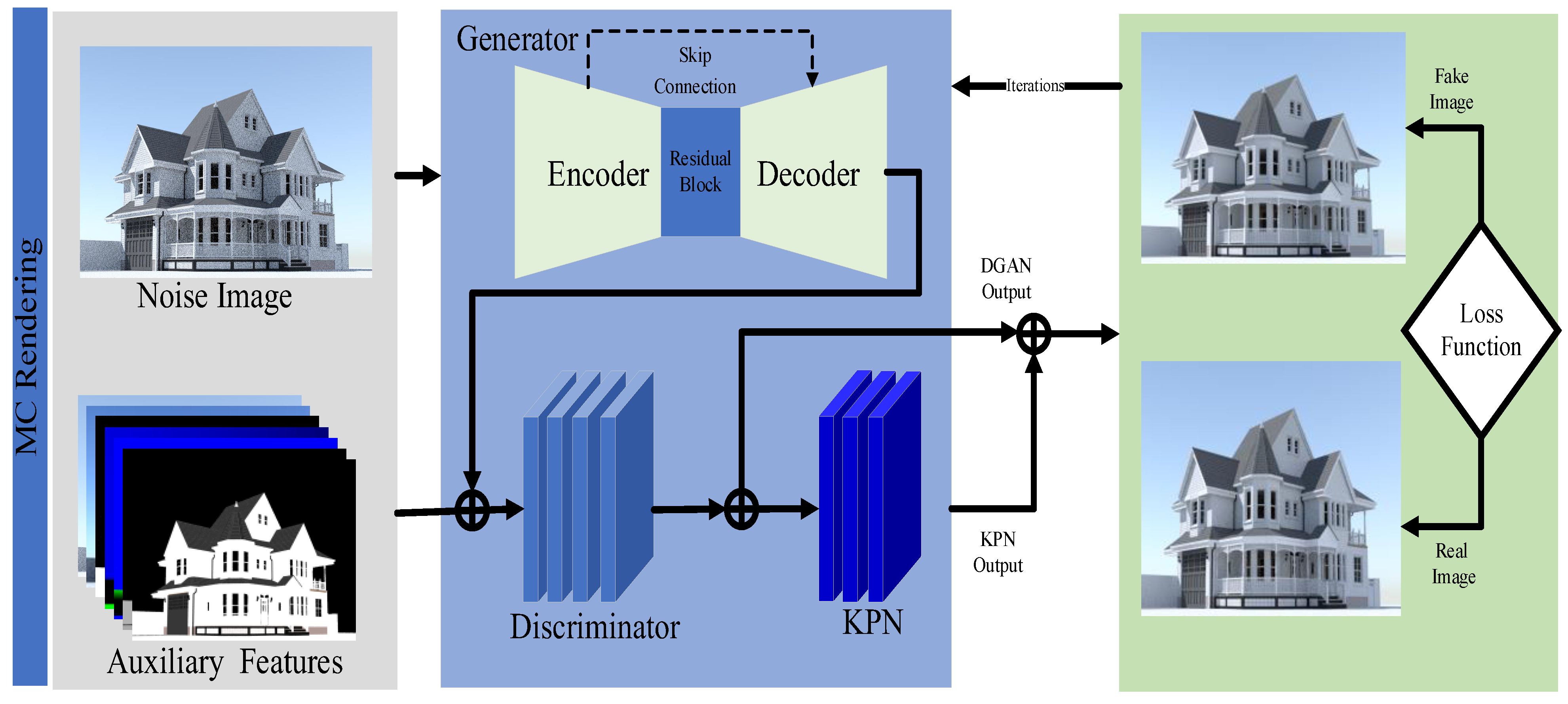
:In this paper, we present a denoising network composed of a kernel prediction network and a deep generative adversarial network to construct an end-to-end overall network structure. The network structure consists of three parts: the Kernel Prediction Network (KPN), the Deep Generation Adversarial Network (DGAN), and the image reconstruction model. The kernel prediction network model takes the auxiliary feature information image as the input, passes through the source information encoder, the feature information encoder, and the kernel predictor, and finally generates a prediction kernel for each pixel. The generated adversarial network model is divided into two parts: the generator model and the multiscale discriminator model. The generator model takes the noisy Monte Carlo-rendered image as the input, passes through the symmetric encoder–decoder structure and the residual block structure, and finally outputs the rendered image with preliminary denoising. Then, the prediction kernel and the preliminarily denoised rendered image is sent to the image reconstruction model for reconstruction, and the prediction kernel is applied to the preliminarily denoised rendered image to obtain a preliminarily reconstructed result image. To further improve the quality of the result and to be more robust, the initially reconstructed rendered image undergoes four iterations of filtering for further denoising. Finally, after four iterations of the image reconstruction model, the final denoised image is presented as the output. This denoised image is applied to the loss function. We compared the results from our approach with state-of-the-art results by using the structural similarity index (SSIM) values and peak signal-to-noise ratio (PSNR) values, and we reported a better performance.
1. Introduction
Due to the continuous development of deep learning methods in recent years, there have been many works using deep learning to denoise ordinary images; therefore, the convolution neural network has been widely used in the research of image denoising. Pathak et al. [1] used an encoder to encode and trained to generate images conditioned on context, in which the encoders learn a representation that is competitive with other models trained with auxiliary supervision, which captures the appearance, the semantics of visual structures, and complete image restoration. Bert et al. [2] showed a dynamic parameter network structure in which the parameters of the kernel are dynamically adjusted according to the input, because it has high flexibility and avoids a large number of increases, with the condition of the model parameters. Bako et al. [3] proposed a denoising algorithm based on convolutional neural networks, which decomposes the image into diffuse reflection and specular reflection. Therefore, the two parts are trained separately. In addition, for image effects that are not reflected in the input features or included in the training data, the results after denoising will appear blurry. Further, using a fixed filter solves the drawback, but the method is still dependent on filtering kernels in a wide range and becomes acceptably field-limited.
Vogels et al. [4] proposed another denoising network structure based on kernel prediction. In this work, they showed three network structures that can be used in different situations. The first network for a single frame of the input image has four parts: a source encoder, a spatial feature extractor, a kernel predictor, and weight reconstruction. The spatial feature extractor includes multiple residual network structure blocks [5]. The second and third network structures are temporal denoisers for multi-frame and multi-standard images. Each frame is first passed through a separate original encoder and spatial feature extractor, and then combined and inputted to the temporal feature extractor and kernel predictor to obtain the final denoised image.
Recently, Mildenhall et al. [6] also proposed a denoising process for images taken with a camera held by a hand, and then using a convolutional neural network structure. This network structure can learn to obtain a kernel that follows spatial changes; the kernel can denoise or register the image, and the trained network has a good denoising effect on most noisy images. Mao et al. [7] proposed a novel deep self-encoding network structure for image restoration. This network has an encoder and a decoder. The encoder and decoder are symmetrical in structure, with convolutional and reversed layers, respectively. In particular, this network also uses skip connections, which can effectively solve the difficulty in deep network training and the problem of gradient disappearance, and can, at the same time, transfer image detail information from the convolutional layer to the deconvolution. The layering helps to build a clear real image. The above work has proven that deep learning has very good performance in image restoration and image denoising.
At present, the use of deep learning methods to denoise the Monte Carlo-rendered images has gradually attracted attention. Unlike general image restoration, in the process of denoising the Monte Carlo-rendered image, in addition to the color information of the pixels, additional auxiliary information can be used, such as depth, normal, and albedo.
The Monte Carlo denoising method of the joint kernel prediction network and generation adversarial network proposed in this paper uses the generation adversarial network to perform preliminary denoising on the Monte Carlo-rendered image, and then applies the prediction kernel output by the kernel prediction network to the preliminary denoising image to obtain the final result. The difference between the method in this paper and the existing kernel prediction Monte Carlo denoising method is reflected in the following aspects [3,4,8]. First, as an improvement of the kernel prediction network method, this paper introduces an adversarial generation network to generate preliminary denoising results and denoise on this basis, instead of directly applying the prediction kernel to the original noisy rendered image. For support, the two work together to assemble the two into an end-to-end denoising network for joint training. Secondly, a loss function is added to support collaborative training of the kernel prediction network and the generative adversarial network to improve the scene detail retention ability and the scene clarity and contrast.
The denoising network in this article is used to process input images with a low sampling rate such as 4 spp, and it can obtain better results. In addition, when constructing the dataset, this article deliberately uses multiple renderers to generate supervised data, which effectively improves the generalization ability of the network. The kernel prediction network in our model takes the auxiliary information images of the Monte Carlo rendering as the input, and the adversarial generation network takes the noisy rendered image itself as the input. This processing method can ensure that each part of the network can encode more image features, thereby capturing more scene details.
In order to further solve the problems of the above two methods and improve the denoising effect of Monte Carlo-rendered images, the main contributions of this paper are the following three points:
- In the first part of this paper, we propose a new end-to-end Monte Carlo denoising rendered image based on the deep learning network structure, and we use the kernel prediction network to optimize the generalization ability of the denoising method for better scene structure and detail retention capabilities.
- We introduce a loss function based on adversarial training to make network training more stable and effective, to improve the clarity and contrast of the denoised image, and to retain more image details.
- We prove that a few auxiliary features can improve the noise reduction effect and solve the loss of high-frequency details of our approach to some extent.
- Our approach is applied to the deep convolutional neural network and makes the learning ability of the network more powerful, with less time-consuming processing.
2. Related Work
In recent years, the Generative Adversarial Network (GAN) [9] has also been shown to achieve good results in image restoration and high-resolution image generation [10,11,12,13,14]. Moreover, generative adversarial networks have also played a role in image denoising works [15]. Regarding the problem of image denoising by Monte Carlo rendering, in 2019, Xu et al. [16] found that the recent Monte Carlo denoising method based on deep learning is more dependent on artificial optimization goals. Therefore, they proposed a method to denoise the Monte Carlo-rendered image by introducing a generative adversarial network. The network then processed the highlights and diffuse components in the rendered image. Finally, the denoised image was output directly and excellent results were obtained. Therefore, the generative adversarial network has considerable potential in the problem of Monte Carlo-rendered image denoising. Unlike the work of Xu et al. [16], Monte Carlo denoising is based on the kernel prediction network, and the generative adversarial network is integrated into the kernel prediction network as a preliminary denoising generation model. In 2019, Xin et al. [17] extracted structure and texture details from auxiliary features in the rendering stage. Then, they used a fusion sub-network to obtain the details map, and finally used the dual-encoder network to denoise MC renderings. However, this method consumes processing time. Ghrabi et al. [8] proposed a network structure with permutation invariance, used a multilayer coding structure to encode sample data to obtain the splat kernel, and then used this check to reconstruct the input image, making their method the best state-of-the-art method that uses the kernel prediction network and is based on samples. Unfortunately, increasing the number of samples increases the time consumption of the method. In 2020, Munkberg et al. [18] suggested extracting the compressed information representation of each sample by separating the sample into a fixed number of sections, called layers. Through a data-based method, this method learns the unique kernel weight of each pixel in each layer and how to filter the composite layer. This adjustment enables the degreaser operation to achieve a good trade-off between cost and quality. In addition, it provides an effective way to control performance and memory properties, because the algorithm table is the number of layers rather than the number of samples. Moreover, via the separation of two-layer samples, the denoiser achieves an interaction rate and produces an image quality similar to that of the larger network.
Again in 2020, Yifan et al. [19] proposed the Adversarial Denoising for MC Renderings network, which used many convoluted dense blocks to extract rich information of auxiliary buffers, and then used these various hierarchical features to modify the noisy features in the residual blocks. Furthermore, they presented the channel mechanism and spatial interest to exploit property dependencies between channels and spatial features.
In 2021, Yu et al. [20] modified the standard self-attention mechanism to the auxiliary feature guided self-attention module to denoising Monte Carlo rendering based on a deep learning network, which effectively involves the complex denoising process.
Generally, Monte Carlo-rendered image denoising based on deep learning is mainly divided into two categories. One is based on methods of the kernel prediction network [3,4], which uses network estimation to generate a prediction kernel and applies this prediction kernel to the noise input to obtain the final denoised image. The other is to directly map the noise input to the high-quality rendered images; the network is used to directly generate the final denoising rendered image. Thus, the key idea of this paper is to combine the strategies of these two methods to build a Monte Carlo-rendered image denoising model. This is because the method based on kernel prediction is effective in the restoration and preservation of scene structure and scene details. However, the adaptability is poor when the denoised renderer of the image is different from the renderer used in the training set, but the network that directly outputs the denoising results will have relatively good generalization ability.
This paper proposes a method to generate realistic rendered images using an end-to-end network structure. First, the renderer is used to render the 3D model at a low sampling per pixel to obtain a low-resolution image. Therefore, the rendering time is relatively short; then, the proposed new image denoising network is used to obtain a high-quality image.
3. The Method
3.1. Model Architecture
In this paper, we propose a new network structure based on the kernel prediction network and the Deep Generation Adversarial Network (DGAN) to build this function. The kernel prediction model alone or the DGAN model with noise input can be used to generate denoised rendered images [3,4,16]. The difference between these two models is that the kernel prediction network first learns the prediction kernel from the input data and then applies the prediction kernel to the pixels of the noise image. The DGAN learns the connection between the noise pixel and the real pixel as the target, and maps the noise pixel to the reference real pixel, thereby directly generating a denoised image close to the real image. The kernel prediction network can restore the scene structure well and retain the details of the scene, and the DGAN-based method can have better generalization ability. The characteristics of these two models inspired this paper to combine the two to obtain a better denoising effect promotion and generalization ability improvement.
Generally, the idea of combining these two models is not complicated, but we have made many improvements to make these networks work together: First, we improved the previous kernel prediction network [3,6,21] and improved the feature encoder, making it have a better ability to capture scene details and have a better adaptability to input data from different renderers. Secondly, the DGAN network structure contains 4 discriminant networks of different scales as discriminators to supervise the encoding of details at different scales. In addition, to improve the reconstruction quality, the result after the prediction kernel reconstruction is used as a new noise image and the network is used again for the second denoising. This process is repeated many times to obtain the final denoised image. Finally, we propose adding a loss function to the network, which can be trained stably while improving the detail retention ability of the denoising results, the sharpness, and the contrast in the final image.
In addition, the loss function must accurately capture the difference between the estimated pixel value and the real pixel value, and it is easy to adjust and optimize. In Section 3.1.4, we introduce the proposed loss function. Finally, to avoid overfitting in our network, we made a dataset that contains a large amount of data. It takes a lot of time and computational cost to make a dataset that contains a large number of real images, noisy images, and auxiliary features.
Figure 1. This network structure consists of three parts: the deep generation adversarial network model, kernel prediction network model, and image reconstruction model.
3.1.1. Deep Generation Adversarial Network (DGAN)
For a deep-generation adversarial network, the generator is divided into three parts, the first part being the encoder. The encoder contains 4 convolutional layers, and each convolutional layer contains convolution, and three operations of instance normalization and ReLu activation. After the encoder, there are several residual blocks and a structure that combines the input and output information [5]. The specific structure of a residual block contains 2 convolutional layers, and each convolutional layer has 512 convolution kernels with a size of and a stride size of 1; similarly, each convolutional layer is composed of four parts: convolution, instance normalization, and ReLu activation. The residual block introduces a skip connection by adding between the convolutional layers. Then, the decoding part is similar to the encoding part. Therefore, the encoding part is upsampling after the output of the fourth convolutional layer and the eighth convolutional layer, and the output of the fourth convolutional layer and the fourth convolutional layer of the decoding part is jointly upsampled through a skip connection. Then, they are combined after upsampling.
To simplify the description in this section, a network layer composed of these three operations is collectively referred to as a convolutional layer. The first convolutional layer contains 64 convolution kernels, the number of output channels is 64, and for each convolution kernel, the size is and the stride size is 2. Similarly, the number of convolution kernels of the second convolution layer and the third convolution layer is 128, 256, and 512, respectively, the size of the convolution kernel is constant , and the stride size is 2.
3.1.2. The Kernel Prediction Network (KPN)
The difference between the kernel prediction network (KPN) and the general method of denoising using neural networks is that the kernel prediction network does not directly output a denoised image, but the kernel predictor estimates a filter kernel of size for each pixel of the noise image, where, in the implementation of this article, . The kernel predictor contains three convolutional layers, each convolutional layer is filled with zeros, the size of the kernel is convolution kernel, the stride size is 1, and the number of output channels of each convolutional layer is . These prediction kernels enter the reconstruction model and the denoising structure of DGAN to generate clean images.
As different input images may be rendered by different renderers or rendering systems, and thus obtained by different samplers or calculation methods, these inputs are likely to have different noise characteristics, and then the network structure must have applicability to these different inputs [8]. As the first part of the encoder, it is proposed to make the network have this applicability, by extracting relatively low-level and common features in the input information to unify complex input information and reduce the impact of different inputs.
Enlarging the size of the convolution kernel helps expand the perceptual domain to obtain more details about the neighborhood information. The output information obtained after the input information passes through these 2 convolutional layers is compared with the original input information through the skip structure as the final output. The introduction of residual blocks in the denoising processing of Monte Carlo-rendered images has been successful in related research work [22]. It has two advantages: First, as the input image is noisy, with many missing pixels and wrong pixel values, the image is very sparse. Therefore, the input is combined before and after through the residual block to obtain more feature information. Second, the residual block can effectively solve the problem of gradient disappearance caused by the excessive depth of the network during the training process, and the convergence of the loss function during the training process can be faster and more stable.
3.1.3. Image Reconstruction
Recall that the pre-denoising image output of the generation network is , the kernel obtained by KPN , where is a matrix, and its row and column elements are marked as . To ensure that the weight range of each kernel falls in the interval [0,1], and the sum is equal to 1 [21], we first use the SoftMax function to normalize:
The meaning of each element in the prediction kernel is the degree of influence of each pixel area in the domain around the pixel . is the set of kernel sizes. Therefore, the final reconstructed image can be calculated as follows [21]:
Through weights normalizing, we can estimate the final color value included in each pixel area in the image, which can greatly reduce the search space of the output estimation value in the denoising process, and avoid phenomena such as the color shift effect. Secondly, normalization can also make the gradient of the weight value relatively stable, avoiding large gradient oscillations caused by the high-dynamic-range characteristics of the input image during the training process.
3.1.4. Loss Function Design
The network proposed in this article is made up of KPN and DGAN. Thus, designing a reasonable loss function is a very important issue that enables these two networks to work together and improve the quality of denoising. Specifically, our loss function consists of three parts.
Generate the loss function : The generator is responsible for using the input noise image to generate a preliminary denoising rendered image, and the discriminator is responsible for comparing the generated image with the real image. Our dataset is , where is the number of denoise elimination iterations. We set it in our work as 4 iterations, and then considering the generator as , and the discriminator is set as . The training process for generating an adversarial network is a process of optimizing the loss function , such as [23]:
During this, the optimization function (Equation (4)) in the optimization process is used to solve the parameter value of each . Thus, reaches the maximum, this is fixed, and then we solve for to minimize .
The generator at this time has the model parameters to produce a reasonable denoised image by Equation (5). On the contrary, we adopt a different general discriminator form [15]. As for the loss function of a single discriminator, instead of letting the discriminator output a probability value to judge the true or false of the sample, L1 is used to measure the loss between the two samples, namely [15]:
Among them, is the total number of pixels in the image, represents the pixel value of the input image , and the corresponding real image pixel is the output obtained as the input of the discriminator. The same principle represents the output obtained by taking the generator output corresponding to as the input of the discriminator. represents the mathematical expectation, which is the average calculation of the loss values calculated for all samples in the dataset.
Equation (6) is only used when training a single adversarial generation network. When KPN and DGAN are trained together, Equation (6) becomes the following form:
The output of the generator becomes the estimated value of the pixel after the prediction kernel obtained by KPN is applied to the output of the generator .
In kernel prediction loss function , the true value of the prediction kernel cannot be obtained, because there is no such label in the dataset. Thus, we use real images for supervision and, at the same time, make the two networks work together. Therefore, is defined as:
Some state-of-the-art studies [16,24,25] found that comparing L1 loss with L2 loss can also reduce speckle noise-like artifacts in the reconstructed image, because L1 is more sensitive to outliers, such as brighter highlights, which have a great influence on error. Compared with L1 loss, L2 loss will be more robust to outliers, which is also confirmed in previous literature. However, L1 loss or L2 loss usually obtained a higher peak signal-to-noise ratio (PSNR) [26], but the result of the blurring of high-frequency components led to a blurry texture. Therefore, it is necessary to adopt other loss functions to compensate for the high-frequency details. Therefore, we add tone loss function . To make the generated denoised image details have better definition, have a better denoising effect on low-contrast and darker noisy images, and improve its contrast, it is subject to the method inspired by [27], added as a new loss function item to improve the denoising effect of the image. has the following form:
Equation (9) is inspired by tone mapping, which can map the pixels in the image from a small range to a larger range so that the picture can be clearer and brighter. It is a common method in image processing. This penalty item can improve the contrast and clarity of the scene. Finally, the overall loss function defines a mixture of the above three terms:
Among them, , we set the balance parameters as 0.003, 0.008, and 0.09, respectively. Typically, by using such a loss function to make the overall network structure work together, it becomes an end-to-end overall structure.
Finally, this article chooses the gradient magnitude similarity deviation as the image noise estimate because it is relative to other indicators such as the Peak Signal-to-Noise Ratio (PSNR) and Structural Similarity Index (SSIM) [21], because it has achieved good results in public databases for image quality evaluation and the calculation speed is relatively fast.
3.2. Auxiliary Feature
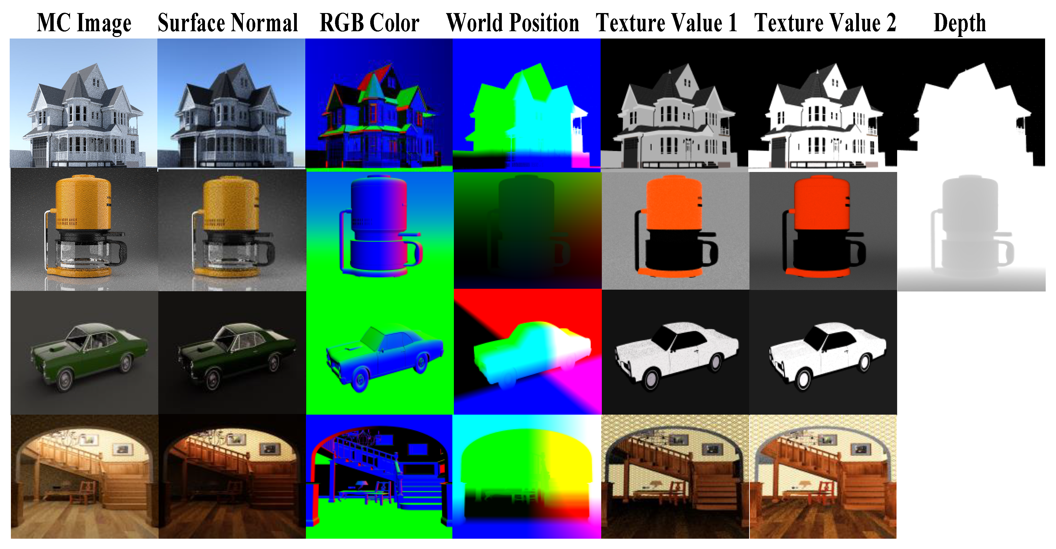
We use the Monte Carlo path-tracing algorithm to render a 3D model, and each pixel needs to shoot a ray from the camera. Then, it records the information when the ray tracer intersects the 3D model for the first time and saves it in the geometry buffer. The saved information includes the texture and material information such as the surface normal, world coordinates, and reflection coefficient of the patch where the intersection point is located, as well as the position of the point in the world coordinate system and the visibility of direct light. This paper does not record information related to a specific scene, such as the position of the light source, intensity, and other attributes of the scene.
The MC images may differ when compared to the ground-truth images, which are clearer and higher-resolution compared to the latter. These differences in training and test data can lead to discrepancies in the actual models. Therefore, it is essential to have datasets that have consistent auxiliary feature images.
Figure 2. The auxiliary feature images include surface normal features (3 channels), RGB color features (3 channels), world position features (3 channels), texture value1 features (3 channels), texture value2 features (3 channels), and the depth feature (1 channel), which contain 13 channels in total, such as the following:
3.3. Dataset and Training
We faced a challenge in the rarity of image datasets, which is hard to find because of the proprietary values. Therefore, crowdsourcing images can be used to address this challenge, and one of the publicly available datasets is the PBRT dataset [28].
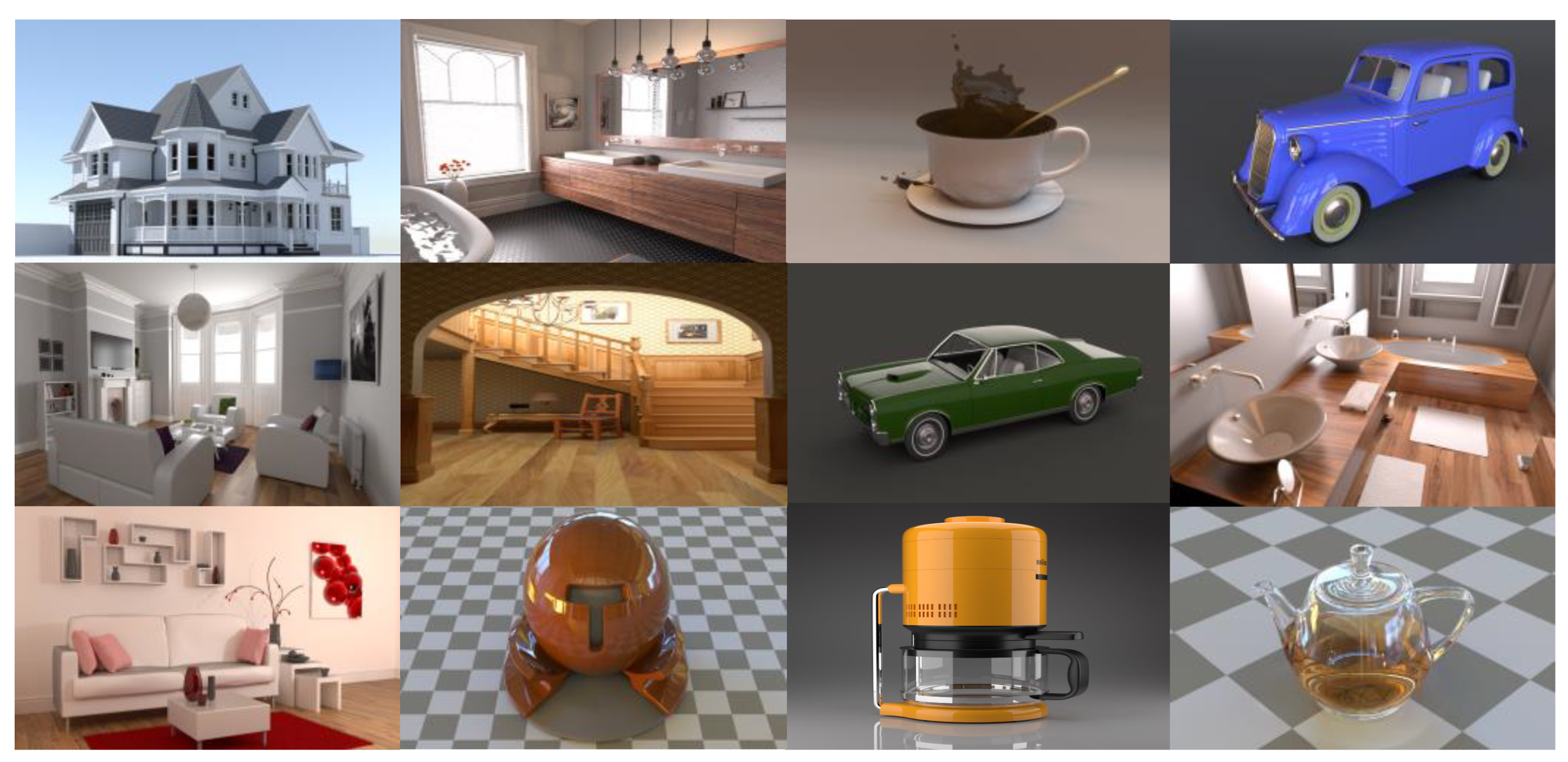
Continuous training of the model involves a large and effective dataset. The training dataset of the state-of-the-art is not public. Therefore, we preferred a reasonably interesting dataset consisting of 21 curated scenes available for use with PBRT [28], which can represent different types of scenes and then modify the environment maps and camera parameters. Therefore, the dataset provides complex scenes that are rendered with 4096 spp such as:
Figure 3 shows examples of reference images rendered with tungsten, and this process is time-intensive, up to several days for some scenes.
In contrast, we divide the training process into two phases. First, the DGAN is trained, including the generator model and the multiscale discriminator model. During training, the standard method in [9] is used to optimize the setting of training parameters, the loss function uses Equation (6) and uses the ADAM optimizer [29], and the parameter settings of the remaining optimizer follow [30] to set the recommended parameters. The initial learning rate is set to 0.0001, the learning rate is fixed before the first 200 epochs, and then the learning rate is gradually reduced according to the linear method. The parameter initialization of the network is initialized with a Gaussian distribution with a mean of 0 and a standard deviation of 0.002, and the batch size is set to 1. Each training iteration will randomly disturb the order of the dataset. Then, KPN is trained, Equation (8) is used as the loss function, and the obtained prediction kernel is applied to the noisy RGB image, rather than against the image generated by the generation network. Using this method makes the training of the kernel prediction network stable. The weights and parameters of the kernel prediction network are initialized using the Xavier method [31], and the bias term is set to 0. The ADAM optimizer is also used, and the parameter and learning rate settings of the optimizer are the same as the province training settings of the generator network model.
The second training process of the overall network structure uses the two networks that have been initially trained. In this training, the number of multiple iterations is set to 4, where the result of the image reconstruction model will be denoised again and then after these repetitions to obtain the final denoising result.
4. Results
This paper proposed using a kernel prediction network and generative adversarial network to construct an end-to-end general denoising network structure, as shown in Figure 1. Our network structure consisted of three parts: the kernel prediction network module, generation adversarial network module, and image reconstruction module. The kernel prediction network module takes the auxiliary feature information image as the input, passes through the source information encoder, the feature information encoder, and the kernel predictor, and finally generates a prediction kernel for each pixel.
The generated adversarial network module is divided into two parts: the generator module and the multiscale discriminator module. The generator module takes the noisy Monte Carlo-rendered image as the input, passes through the symmetric encoder–decoder structure and the residual block structure, and finally outputs the rendered image with preliminary denoising. Then, the prediction kernel and the preliminarily denoised rendered image are sent to the image reconstruction module for reconstruction, and the prediction kernel is applied to the preliminarily denoised rendered image to obtain a preliminarily reconstructed rendered image. To further improve the quality of the result and to be more robust, the initially reconstructed rendered image undergoes four iterations of filtering for further denoising, and the final denoised image is obtained after four iterations of the image reconstruction module as outputs. Finally, this denoised image is applied to the loss function.
We evaluated the denoising MC renderings based on the KPN-DGAN method to solve the MC noise image problem and the high-frequency detail loss.
The PSNR and SSIM matrices were used as the quantitative indicators of denoising results. Thus, PSNR calculated the reconstruction error between the denoised and real images based on the mean square sum (MSE). Note that the errors of these matrices are sensitive to noise; as long as a certain pixel value changes and regardless of which direction it changes, the PSNR will also change. Thus, the value range of PSNR is not fixed, and the maximum value is related to the image resolution.
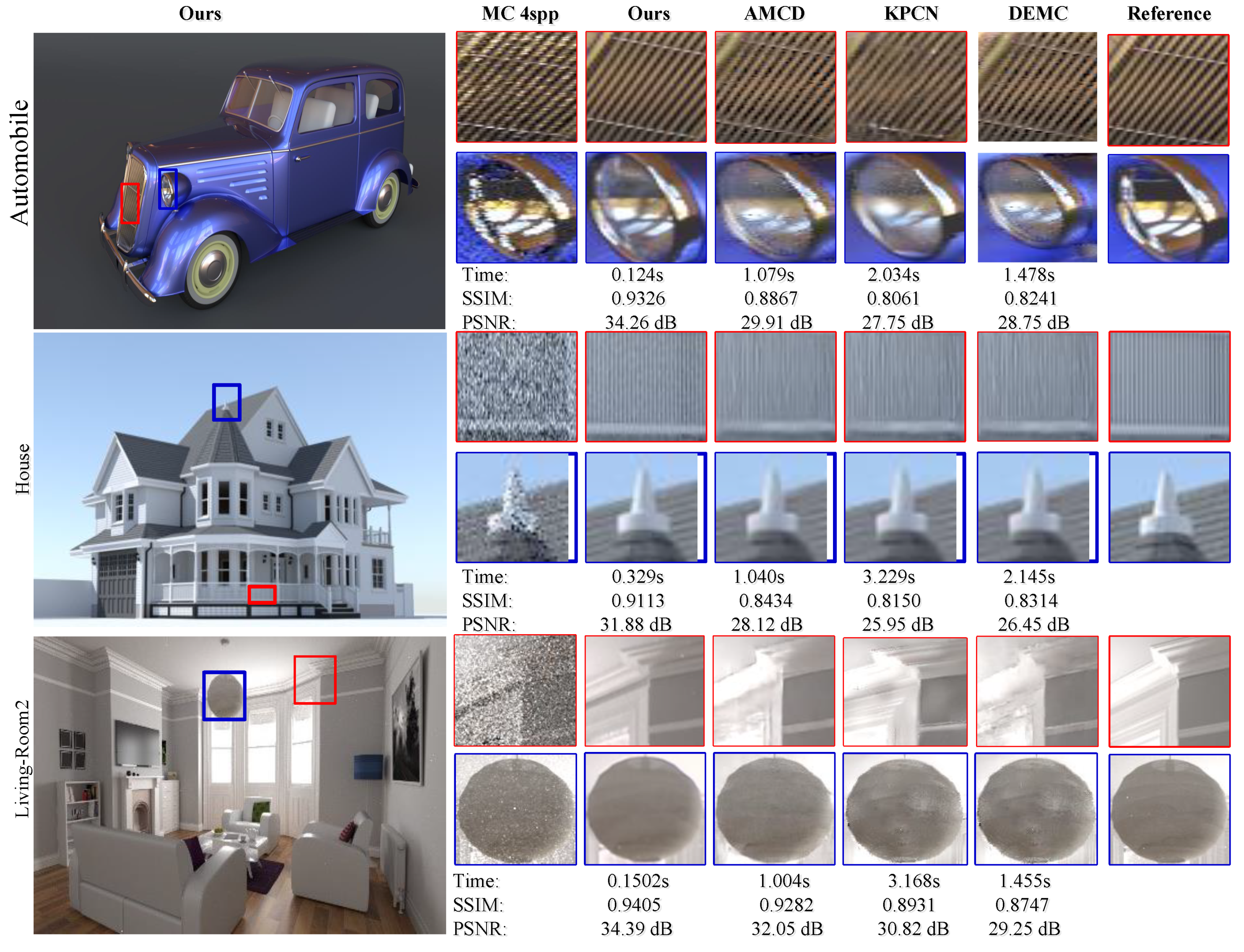
Then, we selected the most representative methods in Monte Carlo image denoising in recent years to compare with our experimental results, which are the KPCN work in 2017 [3], AMCD, and DEMC in 2019 [16,17]. Note that the selected scene uses the 4 spp noise image rendered by the tungsten renderer [32]. The results are as follows:
Figure 4 shows the ablation experiment of this paper, and the enlarged area of image details the MC-rendered image with 4 spp, our result against the AMCD result, KPCN result, DEMC result, and the reference rendered image with 4096 spp. The effect of our approach is better in the final denoising result in terms of subjective details and objective indicators, such as the radiator details and the geometrical objects reflecting sharper on a lamp of the automobile scene, maintaining the barrier shape that does not overlap and the lines in the house scene. In the livingroom2 scene, our method performance is also better and enhances sharp edges with greater detail, unlike other methods. The effect of AMCD algorithms is good, but most of the results are a little blurred. The DEMC and KPCN are poor, because the results have many stains. Generally, comparing the results showed that our approach is better at denoising the MC-rendered image, while retaining and restoring the details and structure of the scene.
The PSNR and SSIM index values are reported under each image, and higher values indicate a better result. The network of our approach performed well and reduced the time consumption of denoising. Therefore, we compared our method against prior methods, with similar processing conditions and an equal sample for all methods, and the results of the average SSIM and PSNR scores are as follows:
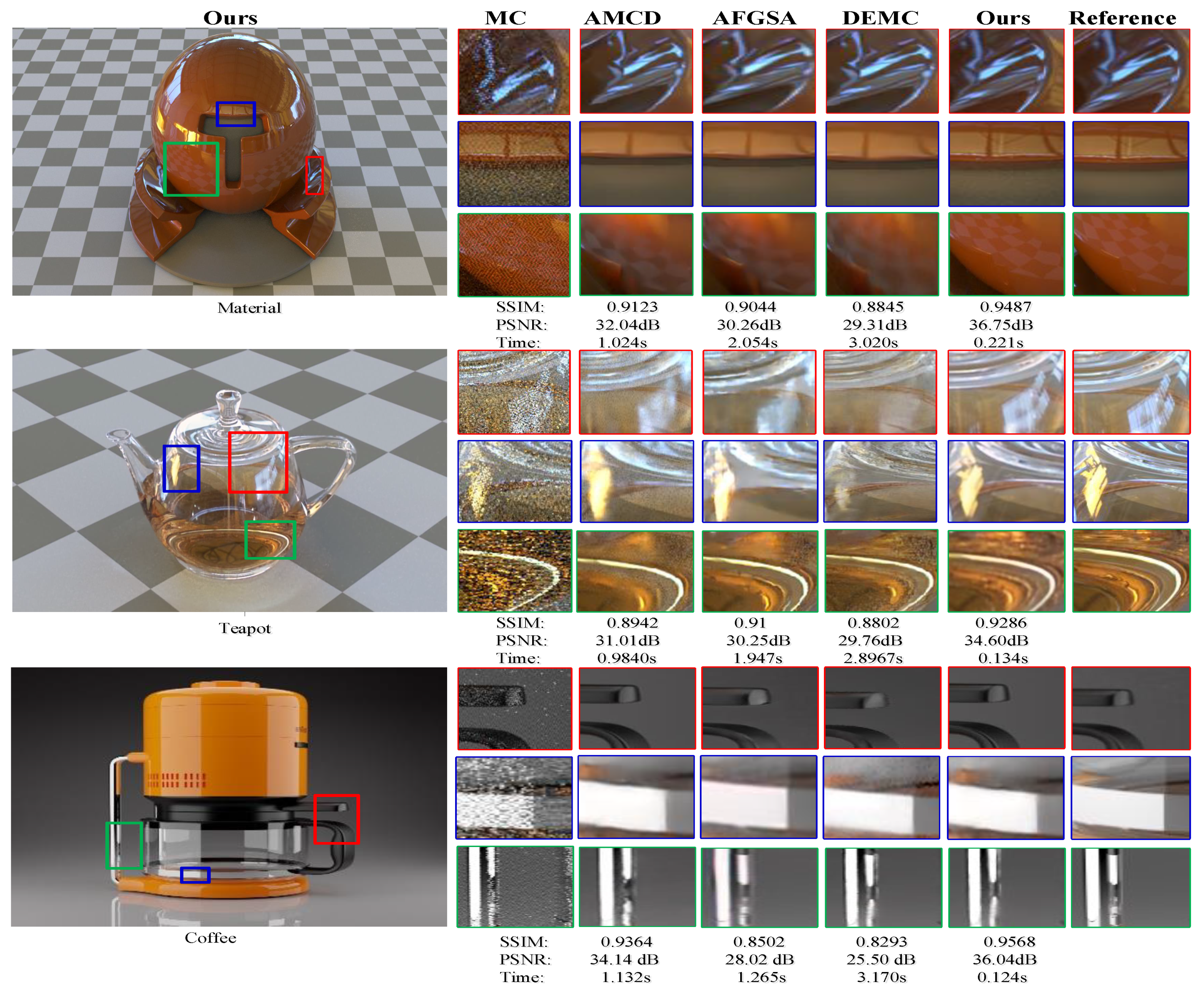
In order to further observe the results of the method in this paper, more scene models were selected for comparison; we highlighted the difference between diffuse and specular components, and the relationship to high-frequency details. Thus, the following comparison experiments were compared with AMCD, the DEMC work in 2019 [16,17], and the AFGSA work in 2021 [20]; all of these techniques have public released codes and weights. The 3D model is still the tungsten renderer, and the sampling rate is 4 spp. The experimental results are as follows:
Usually, the specular and diffuse components have different noise patterns and are highly dependent upon the smoothness or texture of the surface properties. Figure 5 shows the other methods that led to unsatisfactory results, with disturbing effects on material and glass, such as blur region, glossy reflections, depth of field, area lighting, and global illumination. Therefore, they need to take advantage of auxiliary features in different ways. The material scene showed an erroneous texture, the reflected illumination was poor, the teapot scene had blurred details and was smoother, and there was a glow reflection in the glass with more noise in the coffee scene. All methods accepted our approach.
In all noise reduction tests, our method always performed better than several state-of-the-art solutions. Table 1 and Table 2 show the SSIM and PSNR values and time process for all noise reduction results. Accordingly, our method consistently had smaller errors, with higher SSIM values and less time consumption than state-of-the-art methods.
Finally, the KPN-DGAN denoised the Monte Carlo-rendered image with the auxiliary features, which reduced the image noise with a low samples rate, and restored the scene structure details, to improve the quality of rendered images with less time-consuming processing.
5. Discussion
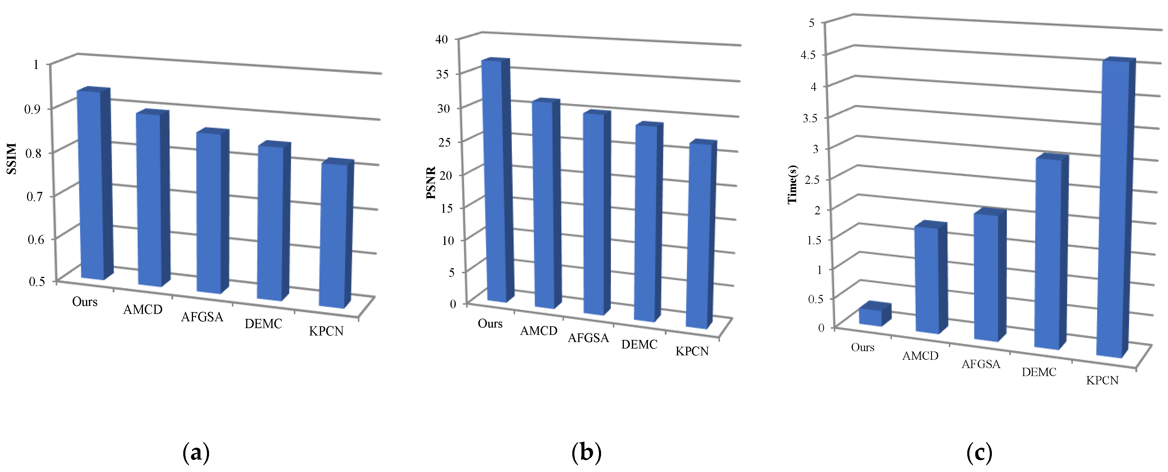
Our main contribution in this approach constitutes a solution for denoising MC renderings trained with a fast deep generative adversarial network, which produces high-quality denoising rendering results with fewer auxiliary buffers, and outperforms state-of-the-art denoising techniques in most situations by saving storage and input/output cost. Furthermore, our approach consistently leads to accurate handling of the diffuse and specular components, in both low-frequency and high-frequency areas, better detail preservation, and a sharp reconstruction to enhance sharp edges with partially saturated pixels and greater detail with less time consumption for rendering. In contrast, the other methods are still time-consuming for denoising in real-time applications even with GPU implementations. The following figure shows the average performance of our work against the baseline of denoising methods KPCN, DEMC, AMCD, and AFGSA.
Figure 6 shows the average performance of our approach against the DEMC, KPCN, AMCD, and AFGSA methods, across test scenes on 4 spp:
In all noise reduction tests, our method is always better than several state-of-the-art solutions. Table 3 shows the aggregate numerical performance of our approach against DEMC, KPCN, AMCD, and AFGSA methods according to the PSNR, SSIM values, and time process for all noise reduction results. Our method consistently has smaller errors, with higher SSIM values and less time consumption than state-of-the-art methods.
Generally, our main contribution in this approach constitutes a solution for denoising MC renderings trained with deep learning, which produces high-quality denoising rendering results with less time-consumption for rendering. In contrast, the other methods are still time-consuming for denoising in real-time applications, even using GPU implementations. On the other hand, KPCN and DEMC successfully denoise most low-frequency areas. Unfortunately, they fail in high-frequency areas, as only stacking the standard convolution operations makes the network lack resilience when facing different auxiliary features, to make the network restore high-frequency information as much as possible. The AFGSA method loses some details and leads to a wrinkle-like artifact, because it is very aggressive at recovering textures and ignores the specular components. Then, the AMCD method adding the adversarial loss is useful to a certain extent, but they produce smooth results at the junction of high/low-frequency areas due to a smoother global illumination effect. Thus, they cannot essentially eliminate this problem and many other effects. However, in Figure 5 on the floor of the material scene, there are soft shadows on the sharp lines, which cannot be filtered while preserving the sharp edges simultaneously. In contrast, our approach consistently leads to accurate handling of the diffuse and specular components, in both low-frequency and high-frequency areas, and better detail preservation and a sharp reconstruction to enhance sharp edges with partially saturated pixels and greater detail. Moreover, our approach uses fewer auxiliary buffers and outperforms state-of-the-art denoising techniques in most situations by saving storage and input/output cost.
6. Conclusions
In this paper, we demonstrated the effect and performance of a kernel prediction network and a deep generative adversarial network to construct an end-to-end general denoising network structure with loss function, and the comparative experiments reflected that our proposed method was effective and had a good denoising effect. In addition, our results were compared with the recent work results of Monte Carlo-rendered image denoising. Accordingly, the comparison results showed that both the visual effects of the image, the measured PSNR, and SSIM showed that our approach had a great improvement against the state-of-the-art. In addition, the denoising effects of the data rendered by multiple renderers showed that the network model of this paper had a relatively good generalization ability and a good adaptability to the rendering data from different rendering systems.
In contrast, to analyze the performance of the method proposed in this paper, we inputted noise images with different sampling rates and compared the denoising effect and running time. The results showed that the method of our approach method achieved better results in terms of effect and running time.
Author Contributions
Conceptualization, A.M.T.A. and C.C.; methodology, A.M.T.A.; software, A.M.T.A.; validation, A.M.T.A.; formal analysis, A.M.T.A.; investigation, A.M.T.A.; resources, C.C.; data curation, A.M.T.A.; writing—original draft preparation, A.M.T.A.; writing—review and editing, A.M.T.A. and C.C.; visualization, A.M.T.A.; supervision, C.C.; project administration, C.C.; funding acquisition, C.C. All authors have read and agreed to the published version of the manuscript.
Funding
This work was supported partially by the National Natural Science Foundation of China under Grant U19A2063 and partially by the Jilin Provincial Science & Technology Development Program of China under Grant 20190302113GX. The authors would like to thank all reviewers for their valuable comments and suggestions.
Institutional Review Board Statement
Not applicable.
Informed Consent Statement
Not applicable.
Data Availability Statement
Not applicable.
Conflicts of Interest
The authors declare that they have no conflict of interest.
Abbreviations
The following abbreviations are used in this manuscript:
| MC | Monte Carlo Method |
| DGAN | Deep Generative Adversarial Network |
| AFGSA | Auxiliary Feature Guided Self-Attention Module |
| KPCN | Kernel Predicting Convolutional Network |
| spp | Samples Per Pixel |
| SSIM | The Structural Similarity Index |
| PSNR | Peak Signal-To-Noise Ratio |
References
- Pathak, D.; Krahenbuhl, P.; Donahue, J.; Darrell, T.; Efros, A.A. Context Encoders: Feature Learning by Inpainting. In Proceedings of the 2016 IEEE Conference on Computer Vision and Pattern Recognition (CVPR), Las Vegas, NV, USA, 27–30 June 2016; Volume 2, pp. 2536–2544. Available online: https://doi.ieeecomputersociety.org/10.1109/CVPR.2016.278 (accessed on 25 November 2021).
- Brabandere, B.D.; Jia, X.; Tuytelaars, T.; Gool, L.V. Dynamic filter networks. In Proceedings of the 30th International Conference on Neural Information Processing Systems, Barcelona, Spain, 5–10 December 2016; pp. 667–675. Available online: https://dl.acm.org/doi/10.5555/3157096.3157171 (accessed on 25 November 2021).
- Bako, S.; Vogels, T.; McWilliams, B.; Meyer, M.; Novák, J.; Harvill, A.; Sen, P.; Derose, T.; Rousselle, F. Kernel-predicting convolutional networks for denoising Monte Carlo renderings. ACM Trans. Graph. 2017, 36, 1–14. [Google Scholar] [CrossRef] [Green Version]
- Vogels, T.; Rousselle, F.; Mcwilliams, B.; Röthlin, G.; Harvill, A.; Adler, D.; Meyer, M.; Novák, J. Denoising with kernel prediction and asymmetric loss functions. ACM Trans. Graph. 2018, 37, 1–15. [Google Scholar] [CrossRef]
- He, K.; Zhang, X.; Ren, S.; Sun, J. Deep Residual Learning for Image Recognition. In Proceedings of the 2016 IEEE Conference on Computer Vision and Pattern Recognition (CVPR), Las Vegas, NV, USA, 27–30 June 2016; pp. 770–778. [Google Scholar] [CrossRef] [Green Version]
- Mildenhall, B.; Barron, J.T.; Chen, J.; Sharlet, D.; Ng, R.; Carroll, R. Burst Denoising with Kernel Prediction Networks. In Proceedings of the IEEE/CVF Conference on Computer Vision and Pattern Recognition (CVPR), Salt Lake City, UT, USA, 18–23 June 2018; pp. 2502–2510. Available online: https://arxiv.org/abs/1712.02327 (accessed on 25 November 2021).
- Mao, X.-J.; Shen, C.; Yang, Y.-B. Image Restoration Using Very Deep Convolutional Encoder-Decoder Networks with Symmetric Skip Connections. Comput. Vis. Pattern Recognit. 2016, 2, 1–9. Available online: https://arxiv.org/abs/1603.09056 (accessed on 25 November 2021).
- Gharbi, M.; Li, T.-M.; Aittala, M.; Lehtinen, J.; Durand, F. Sample-based Monte Carlo denoising using a kernel-splatting network. ACM Trans. Graph. 2019, 38, 125. [Google Scholar] [CrossRef] [Green Version]
- Goodfellow, I. NIPS 2016 Tutorial: Generative Adversarial Networks. arXiv 2016, arXiv:1701.00160. Available online: http://arxiv.org/pdf/1701.00160.pdf (accessed on 25 November 2021).
- Isola, P.; Zhu, J.; Zhou, T.; Efros, A.A. Image-to-Image Translation with Conditional Adversarial Networks. In Proceedings of the 2017 IEEE Conference on Computer Vision and Pattern Recognition (CVPR), Honolulu, HI, USA, 21–26 July 2017; pp. 5967–5976. [Google Scholar] [CrossRef] [Green Version]
- Chen, Q.; Koltun, V. Photographic Image Synthesis with Cascaded Refinement Networks. In Proceedings of the International Conference on Computer Vision (ICCV 2017), Venice, Italy, 22–29 October 2017; pp. 1–10. Available online: https://arxiv.org/abs/1707.09405 (accessed on 26 November 2021).
- Dosovitskiy, A.; Brox, T. Generating images with perceptual similarity metrics based on deep networks. In Proceedings of the 30th International Conference on Neural Information Processing Systems, Barcelona, Spain, 5–10 December 2016; pp. 658–666. [Google Scholar] [CrossRef]
- Gatys, L.A.; Ecker, A.S.; Bethge, M. Image Style Transfer Using Convolutional Neural Networks. In Proceedings of the 2016 IEEE Conference on Computer Vision and Pattern Recognition (CVPR), Las Vegas, NV, USA, 27–30 June 2016; pp. 2414–2423. [Google Scholar] [CrossRef]
- Johnson, J.; Alahi, A.; Fei-Fei, L. Perceptual Losses for Real-Time Style Transfer and Super-Resolution. Comput. Vis. Pattern Recognit. 2016, 9906, 694–711. Available online: https://arxiv.org/abs/1603.08155 (accessed on 15 November 2021).
- Bui, G.; Le, T.; Morago, B.; Duan, Y. Point-based rendering enhancement via deep learning. Vis. Comput. 2018, 34, 829–841. [Google Scholar] [CrossRef]
- Xu, B.; Zhang, J.; Wang, R.; Xu, K.; Yang, Y.-L.; Li, C.; Tang, R. Adversarial Monte Carlo Denoising with Conditioned Auxiliary Feature Modulation. ACM Trans. Graph. 2019, 38, 1–12. [Google Scholar] [CrossRef] [Green Version]
- Yang, X.; Wang, D.; Hu, W.; Zhao, L.-J.; Yin, B.-C.; Zhang, Q.; Wei, X.-P.; Fu, H. DEMC: A Deep Dual-Encoder Network for Denoising Monte Carlo Rendering. J. Comput. Sci. Technol. 2019, 34, 1123–1135. [Google Scholar] [CrossRef] [Green Version]
- Munkberg, J.; Hasselgren, J. Neural Denoising with Layer Embeddings. Comput. Graph. Forum 2020, 39, 1–12. [Google Scholar] [CrossRef]
- Lu, Y.; Xie, N.; Shen, H.T. DMCR-GAN: Adversarial Denoising for Monte Carlo Renderings with Residual Attention Networks and Hierarchical Features Modulation of Auxiliary Buffers. In Proceedings of the SIGGRAPH Asia 2020 Technical Communications, Virtual Event, Korea, 1–9 December 2020; pp. 1–4. [Google Scholar] [CrossRef]
- Yu, J.; Nie, Y.; Long, C.; Xu, W.; Zhang, Q.; Li, G. Monte Carlo denoising via auxiliary feature guided self-attention. ACM Trans. Graph. 2021, 40, 1–13. [Google Scholar] [CrossRef]
- Marinč, T.; Srinivasan, V.; Gül, S.; Hellge, C.; Samek, W. Multi-Kernel Prediction Networks for Denoising of Burst Images. In Proceedings of the 2019 IEEE International Conference on Image Processing (ICIP), Taipei, Taiwan, 22–25 September 2019; pp. 2404–2408. [Google Scholar] [CrossRef] [Green Version]
- Chaitanya, C.R.A.; Kaplanyan, A.S.; Schied, C.; Salvi, M.; Lefohn, A.; Nowrouzezahrai, D.; Aila, T. Interactive reconstruction of Monte Carlo image sequences using a recurrent denoising autoencoder. ACM Trans. Graph. 2017, 36, 1–12. [Google Scholar] [CrossRef]
- Goodfellow, I.J.; Pouget-Abadie, J.; Mirza, M.; Xu, B.; Warde-Farley, D.; Ozair, S.; Courville, A.; Bengio, Y. Generative adversarial nets. In Proceedings of the 27th International Conference on Neural Information Processing Systems—Volume 2, Montreal, QC, Canada, 8–13 December 2014; pp. 2672–2680. Available online: https://dl.acm.org/doi/10.5555/2969033.2969125 (accessed on 26 December 2021).
- Lee, W.-H.; Ozger, M.; Challita, U.; Sung, K.W. Noise Learning Based Denoising Autoencoder. IEEE Commun. Lett. 2021, 25, 2983–2987. [Google Scholar] [CrossRef]
- Fan, L.; Zhang, F.; Fan, H.; Zhang, C. Brief review of image denoising techniques. Vis. Comput. Ind. Biomed. Art 2019, 2, 7. [Google Scholar] [CrossRef] [Green Version]
- Horé, A.; Ziou, D. Image Quality Metrics: PSNR vs. SSIM. In Proceedings of the 2010 20th International Conference on Pattern Recognition, Istanbul, Turkey, 23–26 August 2010; pp. 2366–2369. [Google Scholar] [CrossRef]
- Reinhard, E.; Stark, M.; Shirley, P.; Ferwerda, J. Photographic tone reproduction for digital images. ACM Trans. Graph. 2002, 21, 267–276. [Google Scholar] [CrossRef] [Green Version]
- Bitterli, B. Rendering Resources. 2016, vol. 9. Available online: https://benedikt-bitterli.me/resources/ (accessed on 1 November 2021).
- Kingma, D.P.; Welling, M. An Introduction to Variational Autoencoders. Found. Trends Mach. Learn. 2019, 12, 307–392. Available online: https://arxiv.org/abs/1906.02691 (accessed on 26 November 2021). [CrossRef]
- Zhou, W.; Bovik, A.C.; Sheikh, H.R.; Simoncelli, E.P. Image quality assessment: From error visibility to structural similarity. IEEE Trans. Image Process. 2004, 13, 600–612. [Google Scholar] [CrossRef] [Green Version]
- Glorot, X.; Bengio, Y. Understanding the difficulty of training deep feedforward neural networks. In Proceedings of the Thirteenth International Conference on Artificial Intelligence and Statistics, Sardinia, Italy, 13–15 May 2010; pp. 249–256. Available online: http://proceedings.mlr.press/v9/glorot10a.html (accessed on 27 November 2021).
- Bitterli, B. The Tungsten Renderer. 2014. Available online: https://benedikt-bitterli.me/tungsten.html (accessed on 1 November 2021).
Figure 1.
The overall structure of the proposed method.

Figure 2.
The auxiliary features are rendered with 4 spp; note that in some scenes the depth feature is only white color.
Figure 2.
The auxiliary features are rendered with 4 spp; note that in some scenes the depth feature is only white color.

Figure 3.
Example of our dataset reference images with 4096 spp.

Figure 4.
The comparison of the results of this paper with AMCD, KPCN, and DEMC.

Figure 5.
Comparison of results of our approach against the AMCD, DEMC, and AFGSA results.

Figure 6.
Average performance and time processes of our approach against DEMC, KPCN, AMCD, and AFGSA. The values are relative to the noisy input (a), which shows the performance in the matrix of SSIM, and (b) shows the performance in the matrix of PSNR. Accordingly, higher values of SSIM and PSNR mean better performance. Finally, (c) shows the comparison of processing time for optimization between our approach and other techniques, whereas the lower values of seconds refer to better performance. Note that the highlighted values mean better performance.


Table 1.
The SSIM, PSNR values, and time process results of our approach against the AMCD, KPCN, and DEMC results.
Table 1.
The SSIM, PSNR values, and time process results of our approach against the AMCD, KPCN, and DEMC results.
| Scene | Ours | AMCD | KPCN | DEMC | ||||||||
|---|---|---|---|---|---|---|---|---|---|---|---|---|
| SSIM | PSNR | Time(s) | SSIM | PSNR | Time(s) | SSIM | PSNR | Time(s) | SSIM | PSNR | Time(s) | |
| Automobile | 0.9326 | 34.26 | 0.124 | 0.8867 | 29.91 | 1.079 | 0.8061 | 27.75 | 2.034 | 0.8241 | 28.75 | 1.478 |
| House | 0.9113 | 31.88 | 0.329 | 0.8434 | 28.12 | 1.04 | 0.815 | 25.95 | 3.229 | 0.8314 | 26.45 | 2.145 |
| Living-room2 | 0.9405 | 34.39 | 0.1502 | 0.9282 | 32.05 | 1.004 | 0.8931 | 30.82 | 3.168 | 0.8747 | 29.25 | 1.455 |
Table 2.
The SSIM, PSNR values, and time process results of our approach against the AMCD, DEMC, and AFGSA results.
Table 2.
The SSIM, PSNR values, and time process results of our approach against the AMCD, DEMC, and AFGSA results.
| Scene | Ours | AMCD | AFGSA | DEMC | ||||||||
|---|---|---|---|---|---|---|---|---|---|---|---|---|
| SSIM | PSNR | Time(s) | SSIM | PSNR | Time(s) | SSIM | PSNR | Time(s) | SSIM | PSNR | Time(s) | |
| Material | 0.9487 | 36.75 | 0.221 | 0.9123 | 32.04 | 1.024 | 0.9044 | 30.26 | 2.054 | 0.8845 | 29.31 | 3.020 |
| Teapot | 0.9286 | 34.60 | 0.134 | 0. 910 | 31.01 | 0.984 | 0.902 | 30.76 | 1.947 | 0.8942 | 29.25 | 2.867 |
| Coffee | 0.9568 | 36.04 | 0.124 | 0.9364 | 34.14 | 1.133 | 0.8502 | 28.02 | 1.265 | 0.8293 | 25.50 | 3.170 |
Table 3.
Aggregate numerical performance of all methods.
| Model | PSNR(dB)  | SSIM  | Time(s)  |
|---|---|---|---|
| KPCN | 26.96 | 0.818 | 4.612 |
| DEMC | 28.63 | 0.845 | 3.055 |
| AFGSA | 30.07 | 0.863 | 2.083 |
| AMCD | 31.62 | 0.895 | 1.773 |
| Ours | 36.76 | 0.9361 | 0.2721 |
Publisher’s Note: MDPI stays neutral with regard to jurisdictional claims in published maps and institutional affiliations. |
© 2022 by the authors. Licensee MDPI, Basel, Switzerland. This article is an open access article distributed under the terms and conditions of the Creative Commons Attribution (CC BY) license (https://creativecommons.org/licenses/by/4.0/).
Share and Cite
MDPI and ACS Style
Alzbier, A.M.T.; Chen, C. DGAN-KPN: Deep Generative Adversarial Network and Kernel Prediction Network for Denoising MC Renderings. Symmetry 2022, 14, 395. https://doi.org/10.3390/sym14020395
AMA Style
Alzbier AMT, Chen C. DGAN-KPN: Deep Generative Adversarial Network and Kernel Prediction Network for Denoising MC Renderings. Symmetry. 2022; 14(2):395. https://doi.org/10.3390/sym14020395
Chicago/Turabian StyleAlzbier, Ahmed Mustafa Taha, and Chunyi Chen. 2022. "DGAN-KPN: Deep Generative Adversarial Network and Kernel Prediction Network for Denoising MC Renderings" Symmetry 14, no. 2: 395. https://doi.org/10.3390/sym14020395
Note that from the first issue of 2016, this journal uses article numbers instead of page numbers. See further details here.