
Global Gridded Argo Dataset Based on Gradient-Dependent Optimal Interpolation
by
 , ,
, ,
Chunling Zhang
1 ,
,
Danyang Wang
1,
Zenghong Liu
2,*,
Shaolei Lu
2,*,
Chaohui Sun
2,
Yongliang Wei
1 and
Mingxing Zhang
3 1
College of Marine Sciences, Shanghai Ocean University, Shanghai 201306, China
2
State Key Laboratory of Satellite Ocean Environment Dynamics, Second Institute of Oceanography, Ministry of Natural Resources, Hangzhou 310012, China
3
Ship Management Center, Shanghai Ocean University, Shanghai 201306, China
*
Authors to whom correspondence should be addressed.
J. Mar. Sci. Eng. 2022, 10(5), 650; https://doi.org/10.3390/jmse10050650
Submission received: 4 April 2022
/
Revised: 7 May 2022
/
Accepted: 8 May 2022
/
Published: 10 May 2022
(This article belongs to the Section Physical Oceanography)
Abstract
:The international Argo Program was launched at the turn of the millennium. It has since collected over 2 million vertical profiles of temperature and salinity from the upper 2000 m of the global ocean. Gridded interpolation is a technology that gives full play to the advantages of these profiles because they are scattered. This study develops a global gridded Argo dataset, called GDCSM-Argo, by using an improved gradient-dependent correlation scale method. The dataset is theoretically verified, its error-related statistics are recorded, and it is compared with other datasets to establish its reliability. The results show that the maximum mean RMSEs are 0.8 °C for temperature and 0.1 for salinity, and more than 90% of the analysis results are reliable under the statistical probability of 95%. Not only can GDCSM-Argo adequately preserve large-scale signals in the ocean but also retain more mesoscale features than other gridded Argo datasets. Preliminary applications also verify that GDCSM-Argo can systematically describe the spatio-temporal features of multiple elements in the global ocean, and is a useful tool in many areas of research.
1. Introduction
The “Array for Real-time Geostrophic Oceanography”, known as Argo, is a global observational array of nearly 4000 autonomous profiling floats that was launched in 2000. The aim was to obtain real-time, large-scale, and high-resolution global ocean observational profiles of the upper 2000 m of the ocean [1,2]. By the end of 2007, the initial design of 3000 operational core Argo floats measuring temperature and salinity profiles had been achieved due to a joint effort by more than 30 countries worldwide. Argo continues to provide information on temperature and salinity from the global ocean at a remarkable speed. Over 2 million temperature-salinity profiles gathered by Argo had been made publicly available by November 2020. With more than 140,000 additional profiles every year, the coverage and volume of data from Argo have exceeded all previous traditional observations within two decades, and have improved a large number of nowcasts, forecasts, and projections. The Argo Program has thus been recognized as one of the most successful ocean observation systems in the world [3,4].
The profiling floats used in Argo are freely drifting instruments. This causes the observation profiles collected by them to be randomly distributed in space and time, and significantly limits the use of these data, especially in operational applications. Researchers have been developing applications to deal with the spatio-temporal heterogeneity of observational data since 1980s [5,6,7,8]. Many countries participating in the Argo Program have developed a series of gridded products—e.g., IAP-Argo [9], RG-Argo [10], EN4 [11], BOA-Argo [12], and IPRC-Argo (http://apdrc.soest.hawaii.edu/projects/Argo/data/Documentation/gridded-var.pdf accessed on 10 February 2022). These datasets significantly broaden the range of application of Argo data by homogenizing them in space and time. Most gridded Argo products are constructed by using optimal interpolation or variational analysis.
Determining an appropriate scale for spatial correlation is a key problem in optimal interpolation or variational analysis. Many studies have calculated the deviation between observational information and background information to obtain the variance in the background error and the scale of correlation through function fitting [13,14,15]. This requires sufficiently dense observational data to provide multiple scales of oceanic information. Moreover, the estimated correlation scales used are usually constant. However, the scales of spatial correlation generally vary with the factors used for analysis, direction, and location. To solve this problem, Zhang et al. [16] developed a gradient-dependent correlation scale method (GDCSM, also called gradient-dependent optimal interpolation) based on horizontal changes in the factors of analysis. The structures of the ocean can be described more accurately by a scheme based on an anisotropic correlation scale because it is more flexible and applicable to multi-factor analysis [17,18]. Gradient-dependent optimal interpolation provides an important approach for constructing more accurate gridded Argo products.
Another crucial problem is that most Argo data lack sea surface observations at present. Using the shallowest depth of Argo observations as the surface is one solution to this problem that does not require adding other observational data [19]. For most Argo observational profiles, the difference between the shallowest measurements at 2–5 m and those on the sea surface is non-negligibly different. Another solution is to merge surface observations obtained by traditional means (e.g., XBT, CTD, and TAO) [9,20]. However, far fewer sea surface observations based on traditional means are available than Argo profiles. These sea surface data are expected to be mismatched with Argo observations in terms of quantity and time for the near future. The inversion of surface data corresponding to Argo profiles by using statistical models is thus important.
This study develops an objective system of analysis based on gradient-dependent optimal interpolation and a pycnocline-based model. A global Argo gridded dataset, called GDCSM-Argo, is constructed and applied to analyze the distribution of the global ocean environment. The materials and the methods used in the system for objective analysis are described in Section 2. In Section 3, we verify the gridded dataset GDCSM-Argo and apply it to validate the relationship between fishery and the seawater environment. The advantages of GDCSM-Argo and its special characteristics are discussed in Section 4. Finally, Section 5 summarizes the conclusions of this study.
2. Materials and Methods
2.1. Materials
2.1.1. Argo Observational Profiles
The Argo observational profiles were derived from the China Argo Real-Time Data Center (CARDC, ftp://ftp.argo.org.cn/pub/ARGO/global/ accessed on 30 September 2021). The Argo network has provided global coverage since 2004. We collected Argo observations from 1 January 2004 to 31 December 2020 to generate a monthly gridded dataset. A total of 2,191,788 temperature and salinity profiles were retained after a post-quality-control procedure developed by CARDC [9,21]. These profiles were interpolated to 57 vertical levels (5 m, 10–200 m at 10 m intervals, 220–500 m at 20 m intervals, 550–1250 m at 50 m intervals, 1300–1900 m at 100 m intervals, and 1950 m) by using Akima linear interpolation [22]. The profiles of sound velocity and parameters of the thermocline (mixed layer depth, MLD; thermocline bottom depth, TBD; and thermocline temperature gradient, TTG) were calculated via the T/S profiles by using the formula for sound velocity [23] and the maximum angle method [24].
As shown in Figure 1, more than 50 Argo profiles were obtained within 1° × 1° gridded boxes in most areas of the global ocean from 1 January 2004 to 31 December 2020. More than 100 observational profiles were available for some areas in the Northwest Pacific, the Northwest Atlantic, and the North Indian Ocean. The densities of Argo observations were relatively low in offshore areas and the high-latitude ocean due to the working principle of Argo floats. The analysis here seeks to ensure that more than five profiles were available around each gridded point used for analysis by adjusting the correlation scales. The observational density of Argo profiles was sufficient to meet the requirements of analysis.
2.1.2. Auxiliary Materials
Three categories of gridded Argo datasets were collected to verify our results in this study: RG-Argo, EN4-Argo, and IPRC-Argo. These data are publicly available from the Argo Program Office (https://argo.ucsd.edu accessed on 11 March 2022). RG-Argo, developed by the Scripps Institution of Oceanography, is based on only the observational profiles of Argo by using optimal interpolation. EN4, from the Met Office, was also constructed based on optimal interpolation. IPRC-Argo was developed by the International Pacific Research Center by using 3D variational analysis. Original observations other than those of Argo were added to the latter two datasets.
2.2. Objective Analysis System for Argo
2.2.1. Background Settings
The background represents a preliminary estimate of the value of analysis. The essence of objective analysis or data assimilation is to make several corrections to the background using real-time observations to obtain results close to empirical observations. Therefore, the background is very important, especially in areas with sparse observations or no observational data. In such cases, the results of analysis depend almost entirely on the background.
The gridded dataset developed in this study was based only on Argo observation data, without any other observation or result of numerical simulation. The arithmetic average and traditional optimal interpolation [25,26] were used to construct the background of the subsurface (5–2000 m) temperature, salinity, and sound velocity from Argo. The Argo profiles were first filtered to remove unreliable data and merged into 1° × 1° boxes in the global ocean (179.50° W–179.50° E, 89.5° S–89.5° N). By using this as the first guess, the climatological background was constructed by traditional optimal interpolation. Then, the climatological background was taken as the field of the initial guess and seasonal background values were calculated by using the same method of analysis. Finally, the monthly background was derived from the seasonal average field.
2.2.2. Gradient-Dependent Optimal Interpolation
Gradient-dependent optimal interpolation is an improvement over traditional optimal interpolation with the purpose of obtaining a value of optimal analysis for the goat point based on least-squares theory. The results at the gridded point used for analysis were adopted as the background value plus the observational increments weighted by optimal weights. The standard equation of the influence of M observations on the analysis point is given in Equation (1). A critical part of the scheme involves estimating the optimal weights. According to minimum variance theory, the optimal weight can be determined by solving Equation (2) [26] (pp. 168–203):
where is the analysis value and can be any environmental variable, such as temperature, salinity, or sound velocity. The symbol , given by the Argo monthly background, is the first estimated value. The subscript i denotes the number of gridded points used for analysis, and j and k denote the number of available sites of Argo profiles. For observational increments, , the observational operator H was used to convert the background into the first guesses of the observation . A radial distance was set to ensure that only Argo profiles were located within a specified range surrounding each analysis point. Each increment had an optimal weight associated with the background error correlations and . and are correlations between the background errors at the two observational points, j and k, and at the fishery and observation points i and k, respectively. The parameter is the square of relative observational errors compared with the background errors. It is frequently set to be a constant for a single source of observation and “tuned” to vary the weights of the observations. As shown in Table 1, the root mean-squared error (RMSE) for each factor was at a minimum with η = 0.5 in the global ocean.
The correlations are usually assumed to follow a Gaussian exponential function, and are inversely proportional to the distance [16,17,27], as shown in Equations (3) and (4):
where x and y are the longitude and latitude, respectively, and depends on the Rossby radius of deformation and changes in the horizontal gradient that define the scale of correlation of the background error. The parameter is the scale of correlation that can be obtained from the product of the scale parameter and the cosine function of the latitude at the analysis gridded point. The radial distances were set to 500 km and 1000 km when constructing the climatological and the monthly products, respectively, to ensure that a sufficient number of observations were considered [17,18]. The parameter G, calculated using Argo climatological data, was associated with the horizontal gradient(s) at location i. It contained a zonal component and a meridional component .
By taking temperature as an example, Figure 2 shows the zonal and meridional distributions of the correlation scale at a depth of 100 m, with each small ellipse generated in 3° × 3° boxes. The scales of zonal correlation were different from the meridional scales at each gridded point used for analysis. The correlation scales varied with the horizontal gradient of temperature. In particular in areas of the sea with a large temperature gradient, such as the Kuroshio area, the North Atlantic Gulf Stream, and the subtropical composite area, the scale of temperature correlation was relatively small. It is clear that the Gaussian functions presented in Equations (3) and (4) provide error correlations in the anisotropic background at each point of analysis.
2.2.3. Pycnocline-Based Model
The statistical model used to estimate the surface temperature and salinity was based on the following parameters: the MLD or upper depth of the thermocline, TBD, and TTG [24]. Density profiles were used to calculate the upper depth and bottom depth of the pycnocline, denoted by MLD and TBD, respectively. It is more reasonable to obtain the parameters of the thermocline by density than temperature to avoid the influence of the barrier layers and salinity [28]. These key parameters were determined by the maximum angle method [29,30], and the surface information was constructed by the model depicted in Equations (5)–(7):
where SST and SSS represent the sea surface temperature and salinity, respectively, and indicate the subsurface temperature and salinity at the depth z as estimated by data on the density profile from Argo, respectively, and and are pressures on the sea surface and the subsurface, respectively. SST is significantly affected by the characteristics of the thermocline. Therefore, nine reference layers (5, 10, 20, 30, 40, 50, 80, 100 and 120 m) were selected to calculate the sea surface temperatures by Equations (5) and (6) and were mean-weighted by Equation (7) [28]. The subscripts i and j denote the number of Argo profiles available around the gridded point for analysis and the datum layer. is the weight coefficient and , with the mean value , represents the RMSE of compared with the value obtained by the Global Temperature and Salinity Profile Programme (GTSPP). The parameter L of the correlation scale was set to 2 degrees, as in previous studies [28].
3. Results
3.1. GDCSM-Argo Information
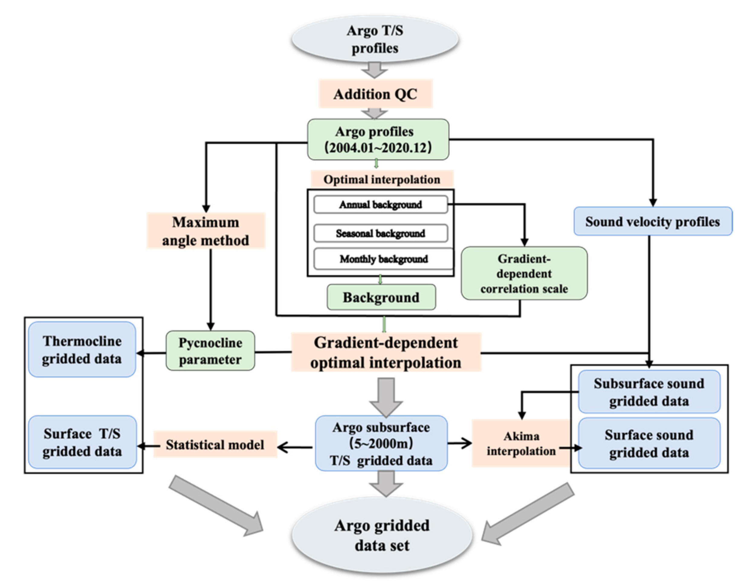
The objective system of analysis for Argo described in Section 2.2 was used to build a global gridded dataset for Argo, called GDCSM-Argo, by using the procedure illustrated in Figure 3. First, the density, sound velocity, and parameters of the thermocline corresponding to each Argo profile were calculated and screened. Second, the gradient-dependent scales of correlation were given by setting the background data via the procedures detailed in Section 2.1.1. Third, objective analysis of the Argo data was carried out based on gradient-dependent optimal interpolation and the global subsurface gridded data of the temperature, salinity, sound velocity, and the gridded parameters of the thermocline was obtained. Finally, the pycnocline-based model was used to construct the surface temperature and salinity. The gridded sound velocity on the surface was determined by the surface temperature and salinity.
The gridded dataset of the GDCSM-Argo covered the global ocean (179.5° W–179.5° E, 89.5° S–89.5° N) from January 2004 to December 2020. The temperature, salinity, sound velocity, depth of the thermocline, its upper and bottom depths, and its temperature gradient were all contained in this production. At a spatial resolution of 1° × 1°, it had several scales of temporal resolution, including each month of the year, the monthly average, seasonal average, and annually averaged climatology. A total of 58 vertical levels were divided at a depth of less than 2000 m.
3.2. Verification
3.2.1. Theoretical Verification
The RMSE is a general index to measure the deviation between the results of analysis and in-situ observations. The quality of the GDCSM-Argo is checked by using the distributions of T/S RMSEs at different depths in Figure 4. The RMSEs at the depths of 5–2000 m were calculated by using the differences between the gridded objective analyses and the merged observations (i.e., the materials described in Section 2.1.1). The T/S RMSEs at the sea surface were obtained by using the surface observations of the GTSPP as the true value. The RMSE of the temperature increased at a depth of 0–150 m and then decreased with increasing depth (Figure 4a). The RMSE of salinity decreased gradually from the surface to the bottom (Figure 4b). At depths greater than 1000 m, the RMSEs of temperature were smaller than 0.2 °C with mean values of 0.05 °C, the RMSEs of salinity were smaller than 0.02 with mean values of 0.01. Above 1000 m, the temperatures and salinities changed more sharply than those deep down due to the impact of surface winds, heat fluxes, and freshwater fluxes. The maximum RMSE of the temperature, about 0.8–1.1 °C, occurred at depths of 100–150 m, where thermocline generally exists. The maximum RMSE of salinity (about 0.12–0.20) occurred near the surface. The RMSEs of both temperature and salinity decreased generally at depths greater than 200 m. All of the temperature and salinity RMSEs are within the theoretical range [31].
The time series of the RMSEs in Figure 5 show that the RMSEs of temperature in different months changed slightly from the surface to a depth of 200 m. The maximum RMSEs of temperature, 0.8–1.1 °C for each month, occurred between 50 and 150 m (Figure 5a). This is similar to the characteristics displayed in Figure 4. At depths greater than 200 m, the RMSEs of temperature gradually decreased (<0.7 °C). The isolines fluctuated at different levels over time. The RMSEs of temperature showed discrepancies between months. In particular in the 24 months from January 2004 to December 2005, the difference in the RMSEs of temperatures in corresponding months of the two years was 0.1 °C. Prominent subsidence in the isolines in August 2012 and November 2017 were also noted. The difference in the RMSEs of temperature was 0.05 °C at the same depth during this period. These differences gradually decreased with increasing depth. The RMSEs of salinity decrease monotonically with increasing depth (Figure 5b). The RMSE of near-surface salinity exceeded 0.15 except in January 2014, but there was little difference between corresponding months of different years. Most of the RMSEs of salinity were less than 0.14 in seawater above 50 m from January 2004 to December 2020. At depths greater than 500 m, all RMSEs of salinity were less than 0.06. Similar to the trend of temperature, the isolines of the RMSE of salinity fluctuated to varying degrees between January 2004 and December 2005, and August 2012 and November 2017. During these months, the RMSEs of salinity were slightly larger than in the corresponding months in the other years considered, where this might have been related to the observation data.
A confidence interval test with a confidence of 0.05 was used to further verify the reliability of the reconstructed dataset by taking the sequence of Argo observations within the effective radius as a sample of the value of analysis [31] (pp. 35–41). At the confidence level, the sample sequence available at most analysis points follows an approximate normal distribution [32]. When statistical variable obeys the distribution with the freedom degree (n − 1). Therefore, the confidence interval of the analysis value on the grid point is , where is for the significance level with a confidence level of 95%. is the available sample sequence within the effective radius, and the corresponding mean value. is the standard deviation.
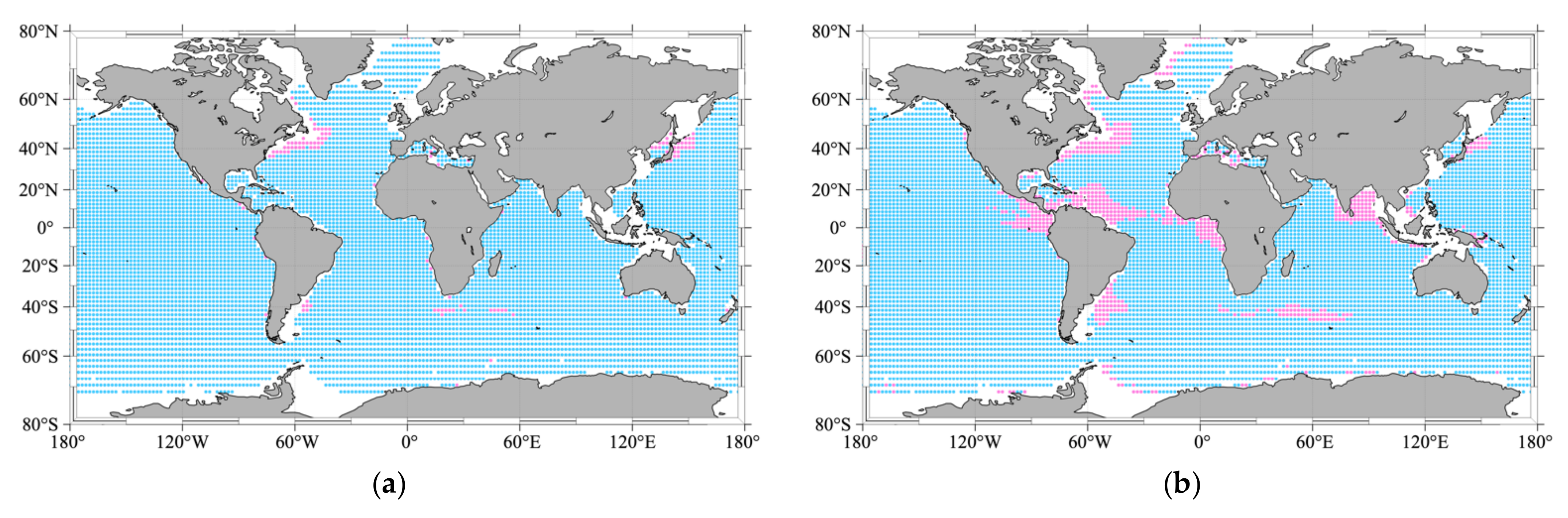
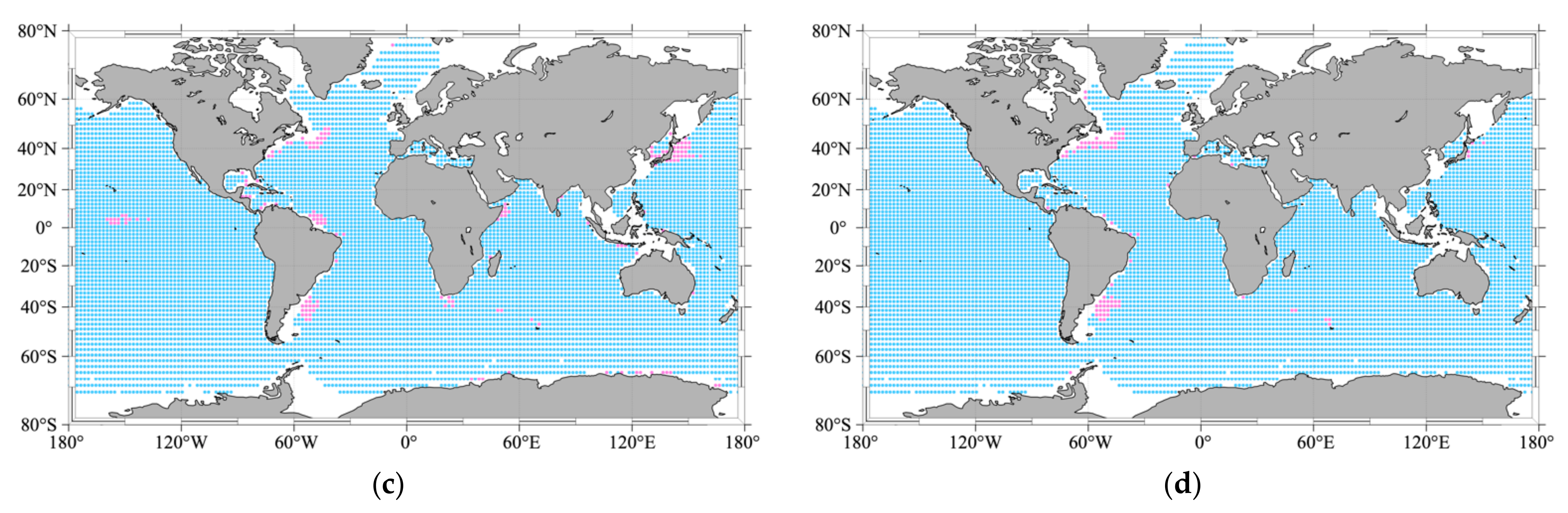
Figure 6 shows the results for annual temperature and salinity at 0 and 150 m. The values marked by blue dots indicate credible values at the gridded points, the results of analysis of which were within their corresponding confidence intervals. In other words, these constructed values were credible with a confidence level of 95%.
Figure 6a,c show that most of the temperature values were credible at a statistical probability of 95%. Only a few values were not within their respective confidence intervals. Even at a depth (e.g., 150 m) with a stark change in temperature, the outlying gridded points did not exceed 10% of the total number of points. These values were mainly located along the boundary areas of the current (e.g., the Gulf Stream, the East Australia Current, and the Kuroshio regions) and regions where the Argo observations were relatively sparse (e.g., near 40° S in the Atlantic Ocean). The number of confidence estimations of salinity at the sea surface yielded more outliers values than those at 150 m, as shown in Figure 6b,d. These points were mostly concentrated along the boundary, near the Equator and the Bay of Bengal. This may be attributed to the transport of their local thermohaline and fresh water flux. Nevertheless, about 90% of the values from the surface analysis were reliable. The credible values increased significantly in number at a depth of 150 m, and a few such points were concentrated along the western boundary of the Atlantic Ocean.
3.2.2. Comparisons against Other Gridded Argo Datasets
Many Argo member countries have developed their own gridded products. The details of several available datasets are shown in Table 2. These datasets have different vertical levels and frequencies of update, but most of them are constructed by optimal interpolation (OI) and are mainly based on the observation profiles of Argo. RG-Argo, developed by the Scripps Institution of Oceanography, and GDCSM-Argo developed in this study are similar in many ways.
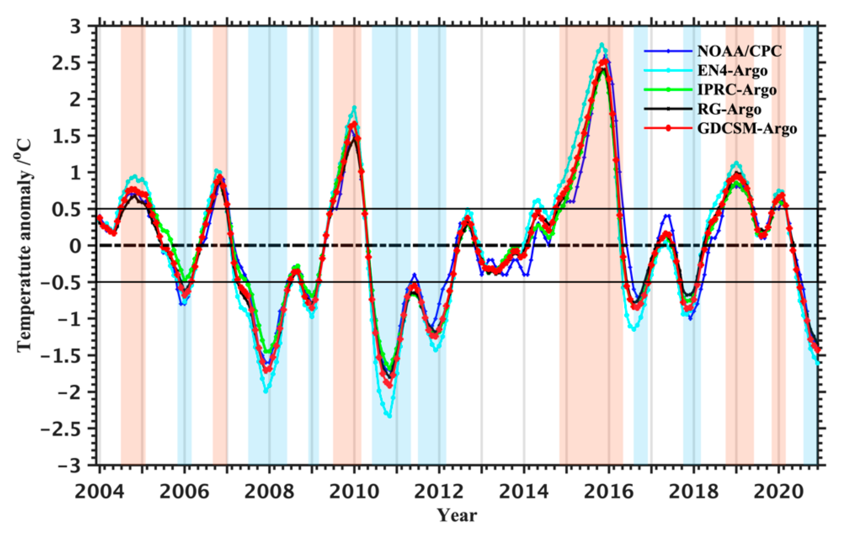
The temporal evolution of El Nino is evaluated in Figure 7 by computing the longitude temporal distribution of anomalies in the vertically averaged temperature at a depth of 0–100 m and the Nino3.4 indices (indices for the intensity of anomalies in the SST in the Central Pacific) by using several kinds of Argo datasets. The Nino3.4 index, derived from the NOAA/CPC (http://www.cpc.ncep.noaa.gov/products/analysis_monitoring/ensostuff/enso-years.shtml accessed on 17 March 2022), was used as the set of standard values. It is clear that the temporal variations in the results of GDCSM-Argo agreed well with those of the other gridded Argo datasets considered. All of them revealed the El Nino-Southern Oscillation (ENSO) events identified during this period by the NOAA/CPC. The ENSO event was marked when the SST anomalies are more than +0.5 °C for El Nino events or less than −0.5 °C for La Nina events within consecutive 3 months [33]. According to this criterion, GDCSM-Argo identifies six El Nino events (2004–2005, 2006–2007, 2009–2010, 2015–2016, 2018–2019, and 2019–2020) and eight La Nina events (2005–2006, 2007–2008, 2008–2009, 2010–2011, 2011–2012, 2016, 2017–2018, and 2020). Moreover, the SST anomalies derived by GDCSM-Argo and RG-Argo have higher consistency with that of NOAA/CPC.
The results of theoretical verification in Figure 6 were used along with a section across the Atlantic Ocean to further verify the gridded GDCSM-Argo data. The differences in T/S among several datasets are given in Figure 8 in comparison with annual data from WOA18 (World Ocean Atlas 2018). Overall, all the differences were smaller than ±2 °C for temperature and ±0.3 for salinity. The mean temperature and salinity deviations between the reference dataset and GDCSM-Argo were the minimum, followed by EN4-Argo, RG-Argo, and IPRC-Argo. Most of the temperature and salinity deviations were smaller than ±0.2 °C and ±0.05 in the results of GDCSM-Argo. The temperature recorded by GDCSM-Argo was 0.5–0.7 °C higher within 0–200 m than that of WOA18 between 25° N and 40° N, and 0.2–0.5 °C lower within 0–500 m between 40° N and 60° N. The salinities of GDCSM-Argo were 0.05–0.10 higher in the subtropical areas, and 0.05 lower in tropical and high-latitude areas than those of WOA18. These colder and warmer structures were also observed in the other three Argo datasets. As mentioned in Table 2, EN4-Argo merged several kinds of historical observations in addition to Argo and adopts used the results of simulation as the background. The differences between EN4-Argo and WOA18 were small. The results of RG-Argo showed similar deviations with WOA18 to those of GDCSM-Argo owing to their similar construction. Their temperature and salinity deviations were ±0.2–0.5 °C and ±0.05–0.1, respectively, significantly larger than those of GDCSM-Argo in many regions. The temperature deviations between IPRC-Argo and WOA18 were the largest among the datasets considered. The temperature recorded by IPRC-Argo was 1.5–2.0 °C warmer in tropical areas and those close to 40°–60° latitude. There were minor deviations in salinity between IPRC-Argo and WOA18.
The temperature and salinity deviations of GDCSM-Argo comparing with RG-Argo are further demonstrated in Figure 9 by using representative stations in the Pacific (150° E, 23° N), the Atlantic (60° W, 30° N), and the Indian (60° E, 45° S) Oceans. The deviations in temperature and salinity were the smallest in the Pacific Ocean, where most of the differences in temperature and salinity were smaller than 0.3 °C/0.04 °C. The differences between particular months (e.g., October 2004, October 2009, and May 2015) slightly increased in the Atlantic. The representative station in the Indian Ocean was in its south, for which the Argo observations were sparse. The deviations in temperature and salinity between certain months in 2004–2008 were about −1.0 °C and 0.1 °C at depths of less than 400 m. A synthesis of the results of three representative stations shows that most of the deviations in temperature and salinity were less than 1.0 °C and 0.1 °C in the global ocean.
3.3. Application
3.3.1. Thermocline Characteristics
The GDCSM-Argo gridded data contained three thermocline parameters: the MLD or upper depth of the thermocline, TBD, and TTG. The MLD can be used to represent the seasonal thermocline, and the TTG is a measure of the seasonal intensity of the thermocline. They had prominent seasonal variations. The characteristics of the MLD in the summer and winter are shown in Figure 10a,b, respectively. In summer, the MLD in the Northern Hemisphere was 0–100 m, significantly shallower than that in the Southern Hemisphere (100–300 m). Part of the MLD was less than 40 m in the area north of 30° N. By comparison, most of the MLD exceeded 150 m, with the maximum depth of more than 300 m, in the area between 40° S and 60° S. Conversely, the winter MLD in the Northern Hemisphere was greater than in the Southern Hemisphere, especially in the area north of 30° N (>150 m) (Figure 10b). Most of the MLD was less than 100 m in the Southern Hemisphere.
The gradients of the thermocline displayed in Figure 10c,d also show significant seasonal variations. Thermocline activity in the Northern Hemisphere was significantly stronger than in the Southern Hemisphere in summer. The TTG in the summer was 0.04–0.20 °C/m in the Northern Hemisphere. Most of the TTG in the Southern Hemisphere was less than 0.05 °C/m in summer. It was greater than 2.0 in the equatorial area of the eastern boundary of the Pacific and Atlantic Oceans. In winter (Figure 10d), the locations where large values (>0.1 °C/m) of the TTG were obtained shift southward, with most of the TTG larger than 0.05 °C/m between 40° S and 20° N. This is similar to the trend in summer, with the highest TTG mainly distributed in the equatorial area.
The correlations among the parameters of the thermocline, MLD, TBD, and TTG, are evaluated in Figure 11 by using annual gridded data in the global ocean. The correlation between MLD and TTG approximately followed a reverse scatter scheme from a numerical point of view. The larger the TTG was, the smaller the MLD was. In other words, the stronger the seasonal thermocline activity was, the shallower was the depth of the mixed layer. Both the TBD and the TTG had the same correlation. There was a positive correlation between the upper and bottom depths of the thermocline (MLD and TBD). Most of the MLD had values (temperature thermocline gradient) of 0.05–0.15 °C/m, with the corresponding MLD and TBD about 10–100 m and 100–500 m, respectively, in the global ocean. All characteristics represented in Figure 10 and Figure 11 are consistent with the results of previous work based on historical observational data.
3.3.2. Global Sound Velocity
The velocity of propagation of sound waves in seawater is affected by temperature, salinity, and pressure. The temperature is the major factor influencing the velocity of sound in the upper ocean. As shown in Figure 12a, the distribution of sound velocity on the sea surface was similar to that of temperature. The surface range of sound velocity was 1460–1550 m/s in the global ocean, with the largest values (>1550 m/s) in the tropical areas, and gradually decreased as the latitude increased. The isolines were distributed in bands. A band of high sound velocity occurred between 20° S and 30° N, with a value greater than 1540 m/s. The velocity of sound decreased to about 1500 m/s near 40° S and 40° N, where the isoline was very dense and almost parallel to the latitude that represents the polar front of sound velocity. The zonal distribution of sound velocity showed two high and three low regions at a depth of 150 m (Figure 12b). High sound velocities, with the values greater than 1520 m/s, were concentrated in the subtropical areas. The band of high sound velocity on the surface in tropical areas was replaced by a sub-high zone, with a range of velocity of 1490–1510 m/s. The velocities were less than 1460 m/s at latitudes were higher than 60°.
Similar characteristics to those detailed above were observed in the section along 180° E, where the isolines of sound velocity were distributed in a “W” shape with changes in the latitude (Figure 12c). The isolines pointed upward in the equatorial areas, downward in the subtropical areas, and were approximately parallel to the latitude between 40° and 60°. They sank more prominently in the Southern Hemisphere than in the Northern Hemisphere. There is an apparent high sound area whose sound velocities are larger than 1540 m/s at the depth of less than 200 m between 20° S and 20° N. The minimum sound velocity (~1470 m/s) occurred in areas at latitudes higher than 60°. The vertical characteristics of sound velocity were clearly exhibited in the tropical section along 0° N (Figure 12d). The velocities were larger than 1540 m/s at depths of 0–100 m. A significant vertical gradient of sound velocity was obtained between 100 m and 150 m in the western boundary of the global ocean. The velocity was 1500 m/s at a depth of 300 m, and decreased to 1480 m/s at a depth of 1000 m. In summary, the structures of the global sound velocity revealed by GDCSM-Argo conformed to expectations.
4. Discussion
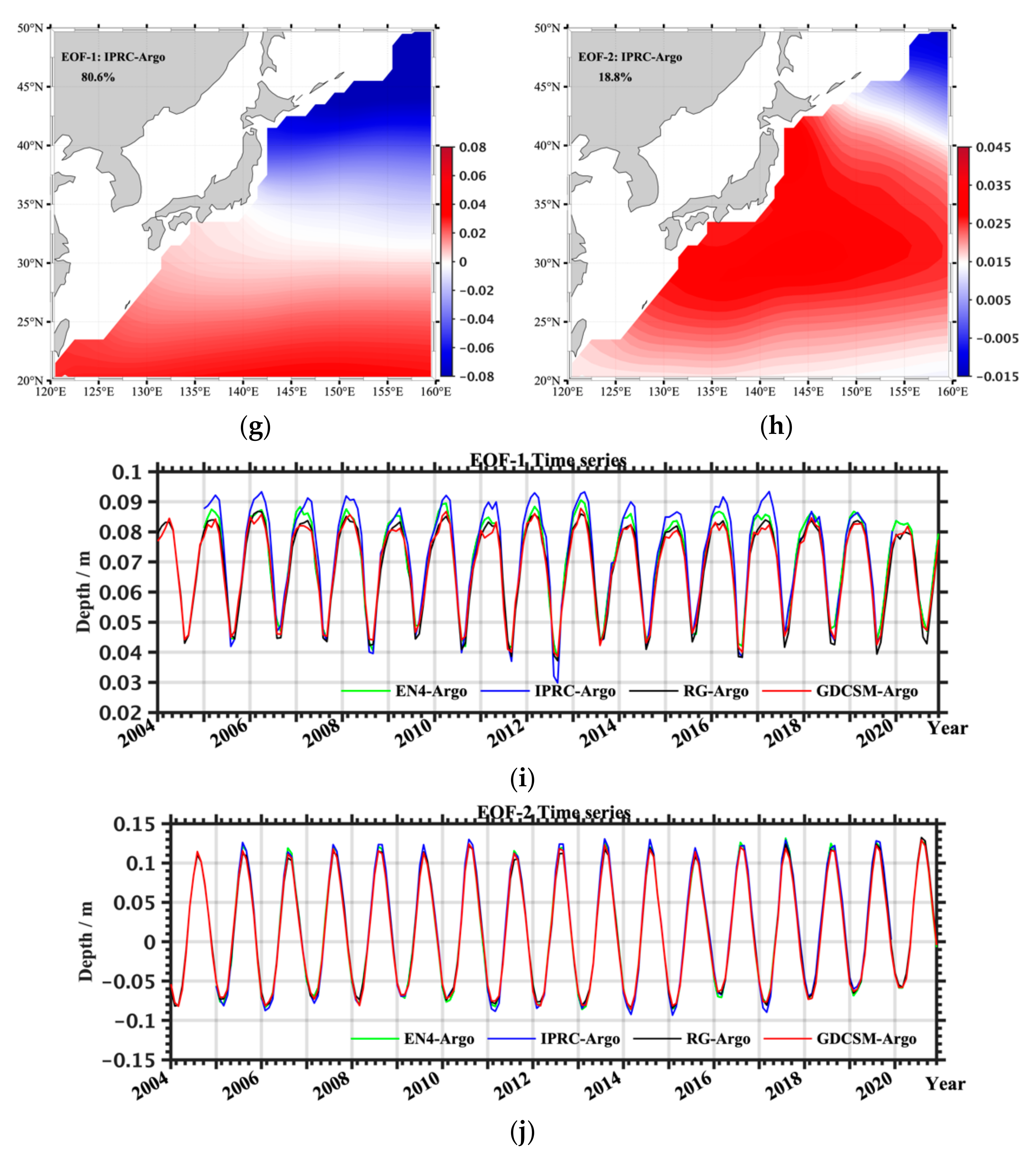
As mentioned in Section 2.2.2, gradient-dependent optimal interpolation gives freely adjustable scales of correlation that are more conducive to obtaining details of changes in the state of the ocean. The capabilities of different kinds of data to extract information on the ocean in the Northwest Pacific are shown in Figure 13 by using the empirical orthogonal function (EOF). Because the divisions of the vertical levels were different, and there was no surface level in some datasets, the temperatures at a depth of 5 m were uniformly used as the near-sea surface temperatures in this section.
All the gridded Argo datasets reflected the mean distribution of temperature in the first (EOF-1) spatial model, with contributions of more than 80%. The EOF-1 models yielded a warm pattern in the south and a cold pattern in the north, with prominent periodic seasonal changes. Variations in the amplitude of the warm south–cold north pattern were more prominent in GDCSM-Argo, with a contribution of 81.8%. Combined with the EOF-1 time series (Figure 13i), the results of GDCSM-Argo yielded the smallest time coefficients, which fluctuated in each cycle. The corresponding spatial model in Figure 13a represents the detailed information. The EOF-1 spatial models of RG-Argo (Figure 13e) and EN4-Argo (Figure 13c) had similar characteristics that were not as evident as those of GDCSM-Argo. The EOF-1 spatial model of IPRC-Argo mainly displayed annual and seasonal signals, with the largest time coefficients.
In addition to the mean pattern, the second mode (EOF-2) revealed the influence of the subtropical anti-cyclone on the near-surface temperature, with contributions of more than 15%. There was a clear warm pattern in the Kuroshio shedding areas between 25° N and 40° N. This had the opposite phase to that of the EOF-1 spatial model. The corresponding series of EOF-2 shown in Figure 13j also had the opposite phase to that of the EOF-1 model but the same cycle. It is clear that the warm patterns in GDCSM-Argo and RG-Argo were very significant, with the smallest time coefficients. Except for the large-scale warm pattern, both GDCSM-Argo and RG-Argo showed more details than the other datasets, which might have been related to their ability to capture meso-scale dynamic processes. Therefore, GDCSM-Argo could extract more detailed signals in areas with large changes in gradient.
5. Conclusions
This study created a gridded Argo dataset called GDCSM-Argo by using gradient-dependent optimal interpolation. The proposed dataset can fully extract patterns of the ocean at multiple scales by using a scheme based on an anisotropic correlation scale. Relative to the original, merged Argo observations, the global mean RMSEs of temperature and salinity were approximately 0.05 °C and 0.01 at depths below 1000 m. The maximum mean RMSEs, with values of 0.8 °C for temperature and 0.1 for salinity, appeared at depths above 200 m, probably due to the impact of surface winds, heat fluxes, and freshwater fluxes. From January 2004 to December 2020, both the temperature and the RMSEs of salinity changed by little over the months. Differences of 0.05–0.1 °C and 0.01–0.02 °C were obtained in the temperature and the RMSEs of salinity in some months, respectively (e.g., January 2004 to December 2005, August 2012, and November 2017). This might have been related to the quantity and quality of the observations. Moreover, more than 90% of the analysis results are reliable under the statistical probability of 95%. All outliers among the gridded points were located in the boundary areas and regions for which Argo observations were relatively sparse. In other words, gradient-dependent optimal interpolation provided reliable results for the global ocean owing to the continual accumulation of observational data.
Comparisons with three gridded datasets, RG-Argo, EN4-Argo, and IPRC-Argo, showed that the results of the proposed GDCSM-Argo were consistent with their analyses in terms of revealing the large-scale interannual patterns of the ocean and the atmosphere. GDCSM-Argo recorded smaller deviations in temperature and salinity than the other gridded datasets in comparison with the annual mean data from WOA18. The maximum temperature and salinity deviations between GDCSM-Argo and WOA18 are no more than 0.5 °C and 0.1 °C. GDCSM-Argo and RG-Argo have good consistency in the global ocean due to the similar background and the observation data. However, there were deviations of 1.0 °C in the temperature and 0.1 in the salinity between the datasets. GDCSM-Argo retained some mesoscale features better than the other gridded Argo datasets because of the anisotropic background-based correlation coefficients of error used in it. It adequately preserved large-scale signals as well as those at meso-scale, and suppressed high-frequency noise.
The gridded dataset developed in this study contains multiple derived factors in addition to the basic temperature and salinity elements. It can systematically describe the spatial characteristics and time series of the global thermocline and the velocity of sound. Both the seasonal thermocline and the permanent thermocline represented in GDCSM-Argo are broadly consistent with those in previous studies. The characteristics of the global sound velocity obtained by it were highly correlated with the temperature of the upper ocean. These findings indicate that GDCSM-Argo is a useful and promising addition to the family of Argo datasets, and can be used in a variety of areas of research. In addition, gradient-dependent optimal interpolation can not only be easily used to construct gridded data without requiring additional computation, but can also be used to generate real-time scattered information on the environment based on observational data. Nevertheless, there are many deficiencies in GDCSM-Argo, e.g., its boundary processing is not detailed enough. We will continue to work on improving GDCSM-Argo and streamline its operational production for near-real-time climate monitoring.
Author Contributions
Conceptualization, C.Z. and Z.L.; data curation, Z.L., S.L. and Y.W.; formal analysis, C.Z.; investigation, C.S. and M.Z.; methodology, C.Z. and S.L.; project administration, Z.L.; validation, D.W., S.L. and C.S.; visualization, Y.W. and M.Z.; writing—original draft, C.Z. and D.W.; writing—review and editing, Z.L., S.L. and C.S. All authors have read and agreed to the published version of the manuscript.
Funding
This research was funded by the National Natural Science Foundation of China under contract nos. 4210060098, U1811464 and 42176012.
Institutional Review Board Statement
Not applicable.
Informed Consent Statement
Not applicable.
Data Availability Statement
The three categories of data used to support the results of this study are included in the article. The Argo profiles were collected from, and are made freely available by, the China Argo Real-time Data Center (ftp://ftp.argo.org.cn/pub/ARGO/global/ accessed on 30 September 2021). The gridded Argo datasets used for verification were provided by the Argo Program Office (https://argo.ucsd.edu accessed on 11 March 2022). The climatic environmental data, gridded data from the World Ocean Atlas 2018 (WOA18), are available from the Ocean Climate Laboratory of NODC (https://www.nodc.noaa.gov/OC5/woa18/ accessed on 1 September 2021).
Acknowledgments
The Argo data were collected and made freely available by the International Argo Program and national programs that contribute to it (https://argo.ucsd.edu; https://www.ocean-ops.org accessed on 15 March 2022). The Argo Program is part of the Global Ocean Observing System. We are grateful to the China Argo Real-Time Data Center for the post-quality-controlled Argo dataset, the Argo Program Office for the gridded Argo datasets, and the National Oceanographic Data Center for providing us with the climate data. We thank H.L. from Fudan University for his technological assistance during the preparation of this manuscript. We thank International Science Editing (http://www.internationalscienceediting.com accessed on 2 April 2022) for editing this manuscript.
Conflicts of Interest
The authors declare no conflict of interest.
References
- Argo Steering Team. On the Design and Implementation of Argo: An Initial Plan for a Global Array of Profiling Floats; International CLIVAR Project Office Report 21. GODAE Report 5; GODAE International Project Office: Melbourne, Australia, 1998; p. 32. [Google Scholar]
- Roemmich, D.; Johnson, G.C.; Riser, S.; Davis, R.; Gilson, J.; Owens, W.B.; Garzoli, S.; Schmid, C.; Ignaszewski, M. The Argo Program: Observing the global oceans with profiling floats. Oceanography 2009, 22, 34–43. [Google Scholar] [CrossRef] [Green Version]
- Wong, A.P.S.; Wijffels, S.E.; Riser, S.C.; Pouliquen, S.; Hosoda, S.; Roemmich, D.; Gilson, J.; Johnson, G.C.; Martini, K.; Murphy, D.J.; et al. Argo data 1999–2019: Two million temperature-salinity profiles and subsurface velocity observations from a global array of profiling floats. Front. Mar. Sci. 2020, 7, 1–23. [Google Scholar] [CrossRef]
- Johnson, G.C.; Hosoda, S.; Jayne, S.R.; Oke, P.R.; Riser, S.C.; Roemmich, D.; Suga, T.; Thierry, V.; Wijffels, S.E.; Xu, J. Argo-Two Decades: Global Oceanography, Revolutionized. Annu. Rev. Mar. Sci. 2022, 14, 379–403. [Google Scholar] [CrossRef]
- Levitus, S. Climatological Atlas of the World Ocean; US Department of Commerce, National Oceanic and Atmospheric Administration: Washington, DC, USA, 1982. [Google Scholar]
- Troupin, C.; Mach, F.; MachOuberdous, F.; Sirjacobs, D.; Barth, A.; Beckers, J.M. High-resolution climatology of the northeast Atlantic using data-interpolating variational analysis (Diva). J. Geophys. Res. 2010, 115. [Google Scholar] [CrossRef] [Green Version]
- Oke, P.; Brassington, G.B.; Griffin, D.A.; Schiller, A. The bluelink ocean data assimilation system (BODAS). Ocean Model. 2008, 21, 46–70. [Google Scholar] [CrossRef] [Green Version]
- Oke, P.; Brassington, G.B.; Griffin, D.; Schiller, A. Ocean data assimilation: A case for ensemble optimal interpolation. Aust. Meteorol. Oceanogr. J. 2010, 59, 67–76. [Google Scholar] [CrossRef] [Green Version]
- Hosoda, S.; Ohira, T.; Nakamura, T. A monthly mean dataset of global oceanic temperature and salinity derived from Argo float observations. JAMSTEC Rep. Res. Dev. 2008, 8, 47–59. [Google Scholar] [CrossRef] [Green Version]
- Roemmich, D.; Gilson, J. The 2004–2008 mean and annual cycle of temperature, salinity, and steric height in the global ocean from Argo program. Prog. Oceanogr. 2009, 82, 81–100. [Google Scholar] [CrossRef]
- Good, S.A.; Martin, M.J.; Rayner, N.A. EN4: Quality controlled ocean temperature and salinity profiles and monthly objective analyses with uncertainty estimates. J. Geophys. Res. 2013, 118, 6704–6716. [Google Scholar] [CrossRef]
- Liu, Z.H.; Li, Z.Q.; Lu, S.L.; Wu, X.; Sun, C.; Xu, J. Scattered Dataset of Global Ocean Temperature and Salinity Profiles from the International Argo Program. J. Glob. Change Data Discov. 2021, 5, 22–31. [Google Scholar]
- Bonekamp, H.G.; Oldenborgh, J.V.; Burgers, G. Variational assimilation of TAO and XBT data in the HOPE OGCM: Adjusting the surface fluxes in the tropical ocean. Geophys. Res. 2001, 106, 16693–16709. [Google Scholar] [CrossRef]
- Hollingsworth, A.; Lonnberg, P. The statistical structure of short-range forecast errors as determined from radiosonde data. Part I: The wind field. Tellus Ser. A-Dyn. Meteorol. Oceanogr. 1986, 38, 111–136. [Google Scholar] [CrossRef] [Green Version]
- Meyers, G.; Phillips, H.; Smith, N.; Sprintall, J. Space and time scales for optimal interpolation of temperature-Tropical Pacific Ocean. Prog. Oceanogr. 1991, 28, 189–218. [Google Scholar] [CrossRef]
- Zhang, C.; Xu, J.; Bao, X.; Wang, Z. An effective method for improving the accuracy of Argo objective analysis. Acta Oceanol. Sin. 2013, 32, 66–77. [Google Scholar] [CrossRef]
- Zhang, C.L.; Wang, Z.F.; Liu, Y. An Argo-based experiment providing near-real-time subsurface oceanic environmental information for fishery data. Fish. Oceanogr. 2021, 30, 85–98. [Google Scholar] [CrossRef]
- Zhang, C.L.; Wang, D.Y.; Wang, Z.F. Fishery analysis using gradient-dependent optimal interpolation. Acta Oceanol. Sin. 2022, 41, 116–126. [Google Scholar] [CrossRef]
- Yan, C.X.; Zhu, J.; Xie, J.P. An ocean reanalysis system for the joining area of Asia and Indian-Pacific ocean. Atmos. Ocean. Sci. Lett. 2010, 3, 81–86. [Google Scholar]
- Martin, M.J.; Hines, A.; Bell, M.J. Data assimilation in the FOAM operational short-range ocean forecasting system: A description of the scheme and its impact. Q. J. R. Meteorol. Soc. 2007, 133, 981–995. [Google Scholar] [CrossRef]
- Li, Z.Q.; Liu, Z.H.; Lu, S.L. Global Argo data fast receiving and post-quality-control-system. In IOP Conference Series: Earth and Environmental Science; IOP Publishing: Bristol, UK, 2020. [Google Scholar]
- Akima, H. A new method for interpolation and smooth curve fitting based on local procedures. J. ACM 1970, 17, 589–602. [Google Scholar] [CrossRef]
- Fofonoff, N.P.; Millard, R.C. Algorithms for Computation of Fundamental Properties of Seawater; UNESCO Technical Papers in Marine Sciences 44; UNESCO: Paris, France, 1983; pp. 3–59. [Google Scholar]
- Chu, P.C.; Fan, C. Maximum angle method for determining mixed layer depth from sea glider data. J. Oceanogr. 2011, 67, 219–230. [Google Scholar] [CrossRef]
- Riishogaard, L.P. A direct way of specifying flow-dependent background error correlations for meteorological analysis system. Tellus A 1998, 50, 42–57. [Google Scholar] [CrossRef]
- Gandin, L.S. Objective Analysis of Meteorological Fields; Gidrometeor Isdaty: Leningrad, Russia, 1963; p. 242. [Google Scholar]
- Kalnay, E. Atmospheric Modeling, Data Assimilation, and Predictability; Cambridge University Press: London, UK, 2003; p. 129. [Google Scholar]
- Zhang, C.; Xu, J.; Bao, X. Gradient dependent correlation scale method based on Argo. J. PLA Univ. Sci. Technol. 2015, 16, 476–483. [Google Scholar]
- Zhang, C.; Zhang, M.; Wang, Z.; Hu, S.; Wang, D.; Yang, S. Thermocline model for estimating Argo surface temperature. Sustain. Mar. Struct. 2022, 4, 1–12. [Google Scholar]
- Wang, X.; Cheng, L.; Zhang, C.; Li, H. Comparative Analysis of Global Applicability of Different Mixed Layer Depth Algorithms. Hai Yang Tong Bao, 2022; accepted. (In Chinese) [Google Scholar]
- Liang, F.Z. Applied Probability and Statistics; Tianjin University Press: Tianjin, China, 2004. [Google Scholar]
- Zhang, C.L. Research on Argo Data Re-Analysis Method and the Re-Construction of Argo Gridded Data Set. Ph.D. Thesis, Ocean University of China, Shandong, China, 2013. [Google Scholar]
- Leetma, A. The interplay of El Nino and La Nina. Oceanus 1989, 32, 30–34. [Google Scholar]
Figure 1.
Number of Argo profiles within 1° × 1° boxes from 1 January 2004 to 31 December 2020 in the global ocean.
Figure 1.
Number of Argo profiles within 1° × 1° boxes from 1 January 2004 to 31 December 2020 in the global ocean.

Figure 2.
The distribution of the temperature correlation scales at a depth of 100 m.

Figure 3.
Flowchart describing the generation of the GDCSM-Argo gridded dataset based on gradient-dependent optimal interpolation.
Figure 3.
Flowchart describing the generation of the GDCSM-Argo gridded dataset based on gradient-dependent optimal interpolation.

Figure 4.
Vertical distributions of the RMSEs of (a) temperature and (b) salinity between the gridded GDCSM-Argo analysis and merged observations at a depth of 0–2000 m over 204 months. The thick black lines represent average values of the RMSE for each variable while the thin gray lines show the monthly RMSEs.

Figure 5.
Time series for RMSEs of (a) temperature and (b) salinity of gridded data from GDCSM-Argo compared with merged observations at a depth above 1000 m. The data are from January 2004 to December 2020.
Figure 5.
Time series for RMSEs of (a) temperature and (b) salinity of gridded data from GDCSM-Argo compared with merged observations at a depth above 1000 m. The data are from January 2004 to December 2020.

Figure 6.
Results of the confidence interval test at a confidence of 0.05: (a) temperature estimations at the sea surface; (b) salinity estimations at the sea surface; (c) temperature estimations at a depth of 150 m; (d) salinity estimations at a depth of 150 m. The blue dots indicate credible gridded point whose results were within the given confidence interval. The red dots represent the opposite.


Figure 7.
Time series of temperature anomalies in the Nino3.4 region (170° W–120° W, 5° S–5° N), based on data from the uppermost 100 m of the ocean, from multiple gridded oceanographic datasets. The anomalies were calculated relative to the annual climatology from the corresponding gridded dataset. The red rectangles indicate El Nino events and the blue rectangles show La Nina events.

Figure 8.
The deviations in temperature and salinity between different datasets and annual data from WOA18 along 30° W. (a,c,e,g) show the differences in temperature between WOA18 and GDCSM-Argo, EN4-Argo, RG-Argo, and IPRC-Argo, respectively. (b,d,f,h) show the corresponding differences in salinity.

Figure 9.
Deviations in temperature and salinity between GDCSM-Argo and RG-Argo gridded datasets. (a,c,e) show the temperature differences at points in the Pacific (150° E, 23° N), the Atlantic (60° W, 30° N), and the Indian (60° E, 45° S), respectively. (b,d,f) show the corresponding differences in salinity.

Figure 10.
The characteristics of the mixed layer depth (MLD) and the temperature thermocline gradient (TTG) in summer and winter in the global ocean: (a) summer MLD; (b) winter MLD; (c) summer TTG; (d) winter TTG.
Figure 10.
The characteristics of the mixed layer depth (MLD) and the temperature thermocline gradient (TTG) in summer and winter in the global ocean: (a) summer MLD; (b) winter MLD; (c) summer TTG; (d) winter TTG.

Figure 11.
Scatter correlation scheme of the parameters TTG and MLD of the annual thermocline, with the corresponding TBD in the global ocean.
Figure 11.
Scatter correlation scheme of the parameters TTG and MLD of the annual thermocline, with the corresponding TBD in the global ocean.

Figure 12.
Annual characteristics of sound velocity (a) on the sea surface, (b) at a depth of 150 m, (c) along the 180° E section, and (d) 0.5° N across the global ocean.
Figure 12.
Annual characteristics of sound velocity (a) on the sea surface, (b) at a depth of 150 m, (c) along the 180° E section, and (d) 0.5° N across the global ocean.

Figure 13.
EOF of near-surface temperature from different gridded Argo datasets in the Northwest Pacific. (a) The first and (b) second spatial model of GDCSM-Argo. (c,d) show models of EN4; (e,f) show the models of RG-Argo; (g,h) show models of IPRC-Argo. The first and second time series are indicated by (i,j), respectively.


Table 1.
RMSEs of temperature and salinity with different value of η.
| Temperature RMSE/°C | Salinity RMSE | |||||||||
|---|---|---|---|---|---|---|---|---|---|---|
| 5 m | 10 m | 100 m | 200 m | 500 m | 5 m | 10 m | 100 m | 200 m | 500 m | |
| η = 0.1 | 0.54 | 0.89 | 0.65 | 0.46 | 0.34 | 0.14 | 0.12 | 0.08 | 0.03 | 0.03 |
| η = 0.25 | 0.46 | 0.80 | 0.61 | 0.50 | 0.32 | 0.13 | 0.13 | 0.07 | 0.04 | 0.03 |
| η = 0.5 | 0.45 | 0.73 | 0.60 | 0.45 | 0.26 | 0.12 | 0.11 | 0.07 | 0.04 | 0.03 |
| η = 1.0 | 0.50 | 0.79 | 0.66 | 0.51 | 0.30 | 0.14 | 0.13 | 0.07 | 0.04 | 0.03 |
| η = 2.0 | 0.59 | 0.84 | 0.73 | 0.53 | 0.37 | 0.19 | 0.16 | 0.08 | 0.05 | 0.03 |
| η = 4.0 | 0.66 | 0.92 | 0.79 | 0.59 | 0.40 | 0.23 | 0.18 | 0.09 | 0.05 | 0.04 |
Table 2.
Information on GDCSM-Argo and other gridded Argo datasets for comparison.
| Dataset Name | EN4-Argo | IPRC-Argo | RG-Argo | GDCSM-Argo |
|---|---|---|---|---|
| Area | 180° W–180° E, 83° S–89° N | 180° W–180° E, 90° S–90° N | 179.5° W–179.5° E, 64.5° S–79.5° N | 179.5° W–179.5° E, 89.5° S–89.5° N |
| Resolution | 1° × 1° | 1° × 1° | 1° × 1° | 1° × 1° |
| Levels | 5–5350 m, 42 levels | 0–2000 m, 27 levels | 2.5–1975 m, 58 levels | 0–1975 m, 58 levels |
| Time | January 1999~December 2021 | January 2005~December 2020 | January 2004~February 2022 | January 2004~December 2020 |
| Observation | WOD05, Argo, GTSPP, ASBO | Argo, Aviso | Argo | Argo |
| Background | Provided by FOAM mode | Provided by mode simulation | Obtained by interpolation | Obtained by interpolation |
| Method | OI | Variation | OI | Gradient-dependent OI |
| Institution | Met Office | International Pacific Research Center | Scripps Institution of Oceanography | Shanghai Ocean University, China Argo Real-time Data Center |
Publisher’s Note: MDPI stays neutral with regard to jurisdictional claims in published maps and institutional affiliations. |
© 2022 by the authors. Licensee MDPI, Basel, Switzerland. This article is an open access article distributed under the terms and conditions of the Creative Commons Attribution (CC BY) license (https://creativecommons.org/licenses/by/4.0/).
Share and Cite
MDPI and ACS Style
Zhang, C.; Wang, D.; Liu, Z.; Lu, S.; Sun, C.; Wei, Y.; Zhang, M. Global Gridded Argo Dataset Based on Gradient-Dependent Optimal Interpolation. J. Mar. Sci. Eng. 2022, 10, 650. https://doi.org/10.3390/jmse10050650
AMA Style
Zhang C, Wang D, Liu Z, Lu S, Sun C, Wei Y, Zhang M. Global Gridded Argo Dataset Based on Gradient-Dependent Optimal Interpolation. Journal of Marine Science and Engineering. 2022; 10(5):650. https://doi.org/10.3390/jmse10050650
Chicago/Turabian StyleZhang, Chunling, Danyang Wang, Zenghong Liu, Shaolei Lu, Chaohui Sun, Yongliang Wei, and Mingxing Zhang. 2022. "Global Gridded Argo Dataset Based on Gradient-Dependent Optimal Interpolation" Journal of Marine Science and Engineering 10, no. 5: 650. https://doi.org/10.3390/jmse10050650
Note that from the first issue of 2016, this journal uses article numbers instead of page numbers. See further details here.