
Teleseismic Indication of Magmatic and Tectonic Activities at Slow- and Ultraslow-Spreading Ridges

1
Key Laboratory of Submarine Geosciences, Second Institute of Oceanography, Ministry of Natural Resources of the People’s Republic of China, Hangzhou 310012, China
2
Institut de Physique du Globe de Paris, Université Paris Cité, 75005 Paris, France
3
Donghai Laboratory, Zhoushan 316021, China
*
Authors to whom correspondence should be addressed.
J. Mar. Sci. Eng. 2024, 12(4), 605; https://doi.org/10.3390/jmse12040605
Submission received: 1 March 2024
/
Revised: 22 March 2024
/
Accepted: 22 March 2024
/
Published: 30 March 2024
(This article belongs to the Special Issue Morphological Processes and Evolution of Marine Geomorphology: Observations, Modeling and Applications)
Abstract
:Magmatic and tectonic processes in the formation of oceanic lithosphere at slow–ultraslow-spreading mid-ocean ridges (MORs) are more complicated relative to faster-spreading ridges, as their melt flux is overall low, with highly spatial and temporal variations. Here, we use the teleseismic catalog of magnitudes over 4 between 1995 and 2020 from the International Seismological Center to investigate the characteristics of magmatic and tectonic activities at the ultraslow-spreading Southwest Indian Ridge and Arctic Gakkel Ridge and the slow-spreading North Mid-Atlantic Ridge and Carlsberg Ridge (total length of 14,300 km). Using the single-link cluster analysis technique, we identify 78 seismic swarms (≥8 events), 877 sequences (2–7 events), and 3543 single events. Seismic swarms often occur near the volcanic center of second-order segments, presumably relating to relatively robust magmatism. By comparing the patterns of seismicity between ultraslow- and slow-spreading ridges, and between melt-rich and melt-poor regions of the Southwest Indian Ridge with distinct seafloor morphologies, we demonstrate that a lower spreading rate and a lower melt supply correspond to a higher seismicity rate and a higher potential of large volcano-induced seismic swarms, probably due to a thicker and colder lithosphere with a higher degree of along-axis melt focusing there.
1. Introduction
The mid-ocean ridge (MOR) is the birthplace of the oceanic lithosphere that covers 2/3 of the Earth’s surface, which is one of the largest volcanic and earthquake belts on the Earth. Earthquakes at the MOR are mainly caused by brittle deformations associated with either tectonic or magmatic activities [1,2,3,4,5]. Earthquakes resulting from tectonic activities, i.e., faulting, may exhibit a relatively stable incidence of occurrence over a long period, while earthquakes triggered by magma intrusions or volcanic eruptions manifest as seismic swarms, characterized by a local and intense occurrence of numerous seismic events over a short period [4,6], which builds volcanic edifices on the seafloor. For example, a seismic swarm triggered by a volcanic eruption in 1999 at 85° E of the Gakkel Ridge consisted of approximately 200 earthquakes over 8 months, with an average magnitude of 4.5 [5,7,8].
As the spreading rate or melt flux of the MOR decreases, the lithosphere tends to be colder and thicker, generally resulting in a deeper and more complex seismicity pattern [9,10,11,12]. Slow- (a full spreading rate of <) and ultraslow-spreading ridges (<) generally have an overall low melt flux and thus a thick lithosphere [13,14,15,16,17], and the interval of the volcanic eruptions of these ridges can be up to thousands of years [18]. Therefore, seismic observations over a short period or a small area, using such as ocean bottom seismometer (OBS) [1,19,20] and autonomous underwater hydrophone (AuH) [2,3,21,22,23], can be limited at slow–ultraslow-spreading ridges. In contrast, teleseismic observations based on land seismic stations can be useful to reveal the overall characteristics of magmatic and tectonic activities of the MOR for a longer period (up to >50 years), although the location error of the teleseismicity could be >10 km and small-magnitude (<4) earthquakes are nearly unobservable. Bergman and Solomon [24] investigated teleseismicity between 1965 and 1989 along the slow-spreading Mid-Atlantic Ridge (MAR) and identified 34 seismic swarms that are associated with volcanic eruptions, suggesting that teleseismicity is an indicator of volcanic activities at the MOR. Schlindwein [4] analyzed the teleseismic catalog between 1976 and 2010 for the ultraslow-spreading Southwest Indian Ridge (SWIR) and Gakkel Ridge (GR), and identified 27 seismic swarms also related to volcanic eruptions. In the subsequent years between 2011 and 2020, numerous earthquakes were observed along slow–ultraslow-spreading ridges, accounting for almost 50% of the earthquakes observed between 1995 and 2020. Particularly, several large seismic swarms occurred at the SWIR with earthquakes numbering >200 between 2016 and 2018. Therefore, updating the study of teleseismicity for slow–ultraslow-spreading ridges is beneficial for understanding their magmatic and tectonic activities as well as associated seafloor morphologies.
In this study, we use the teleseismic catalog between 1995 and 2020 from the International Seismological Center (ISC). This catalog is chosen for events occurring within 35 km off the ridge axis of the slow-spreading North Mid-Atlantic Ridge (NMAR) and the Carlsberg Ridge (CR) and the ultraslow-spreading SWIR and GR, with a total length of the ridge axis of ~14,300 km (Figure 1). We analyze spatiotemporal variations in the earthquakes over a magnitude of 4 (Figure 2), and perform a single-link cluster analysis technique [25] to identify seismic swarms excluding mainshock–aftershock sequences. These analyses allow us to systematically explore the relationship between seismic swarms, volcanic eruptions, and seafloor morphologies, and investigate the dependence of the pattern of seismicity on the spreading rate and the regional melt supply.
2. Data and Methods
2.1. Earthquake Selection
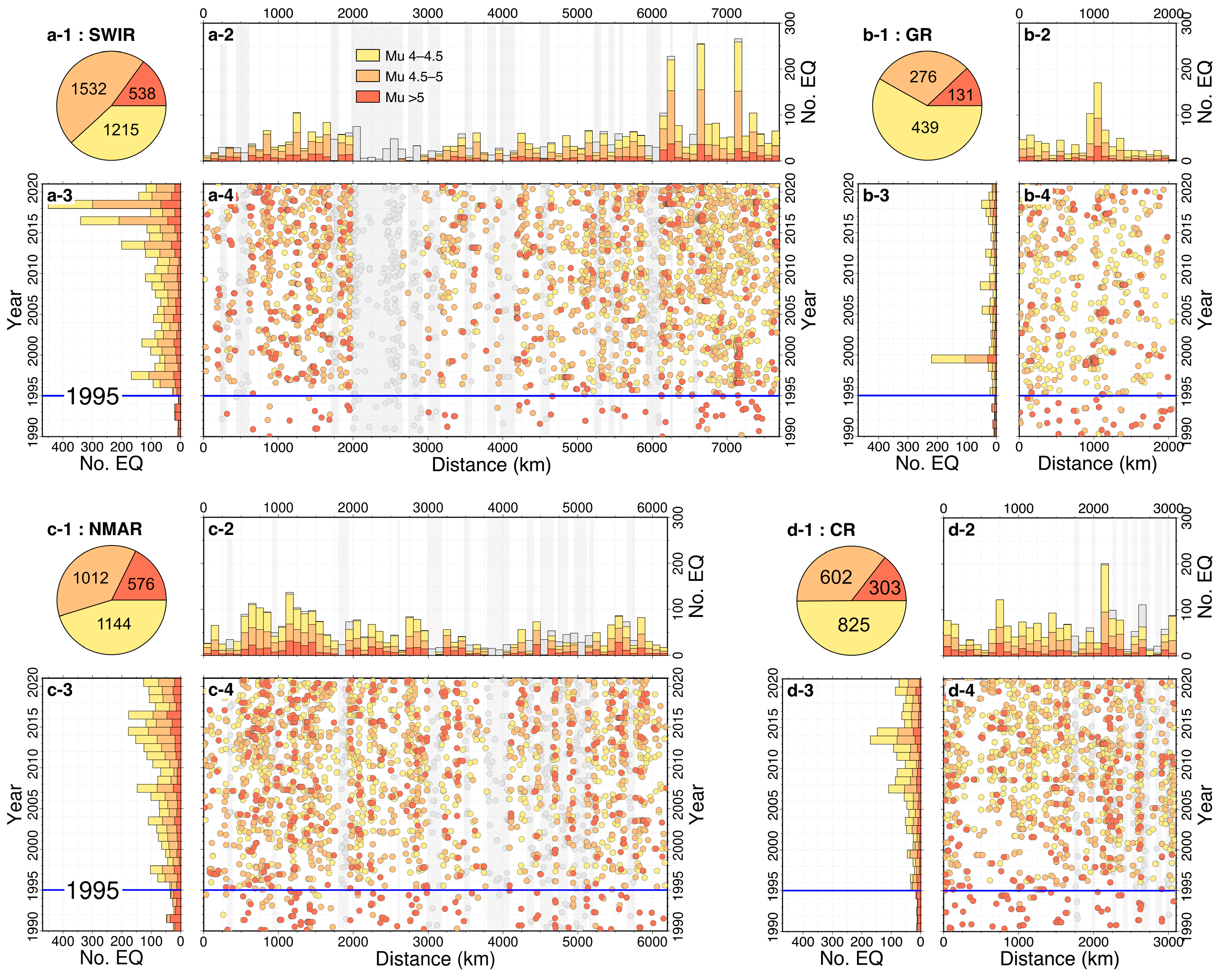
The seismic catalog, including ~700,000 earthquakes, was downloaded from the ISC (www.isc.ac.uk, accessed on 5 March 2022), which has earthquakes of magnitude over 3 between 1990 and 2020 with a horizontal resolution of approximately 10 km (Figure 1a). We selected seismic events within 35 km on both sides of the ridge axes (excluding transform faults) of two ultraslow-spreading ridges (SWIR and GR) and two slow-spreading ridges (NMAR and CR) (Figure 1b–e). The selected earthquake catalog contains 8593 earthquakes, with magnitudes over 4 between 1990 and 2020. We projected the earthquakes vertically onto the ridge axes and displayed them by axial distance (Figure 3). For the SWIR (Figure 3(a-1–a-4)) and GR (Figure 3(b-1–b-4)), the westernmost point was defined as the starting point (distance = 0), and their ridge axes were plotted from west to east. For the NMAR (Figure 3(c-1–c-4)) and CR (Figure 3(d-1–d-4)), the northernmost point was defined as the starting point, and their ridge axes were plotted from north to south.
2.2. Magnitude Unit Normalization
Due to various magnitude scales (, etc.) in the ISC catalog, we unified the magnitude to facilitate statistical analysis [27]:
Then, we derived the seismic moment [28], in the unit of Nm, for each event based on the unified magnitude , using:
By analyzing the completeness magnitude (Mc) of earthquakes, we obtained the Mc of 4.3 for the whole selected earthquake catalog, with Mc of four MORs ranging between 4.0 and 4.3 (Figure 2). Additionally, since the improvement of the global seismic network in 1995 with more stations, new instruments, and better monitoring and data processing technologies, the accuracy and threshold of earthquake detection were greatly improved. Therefore, our analysis in this paper focuses on the post-1995 earthquake data with magnitudes over 4. Earthquakes are divided into three types regarding their magnitudes: 4–4.5, 4.5–5, and above 5 (pie charts in Figure 3). The distribution of earthquake magnitudes at the four MORs is broadly similar, with ~80% of earthquakes at magnitudes of 4–5 and ~20% at over 5.
At the 5200 km-long SWIR, a total of 3221 earthquakes with a magnitude over 4 occurred within 35 km off-axis between 1995 and 2020 (Figure 3(a-1–a-4)), and the seismicity rate (i.e., annual average number of earthquakes per 100 km) is , with an average magnitude of 4.6 (average seismic moment released ). The seismic strain rate is . For the 2050 km-long GR between 7° W and 102° E (Figure 3(b-1–b-4)), there are 800 earthquakes, and the seismicity rate is , with an average magnitude of 4.5 (average seismic moment released ). The seismic strain rate is (Table 1).
For the 4500 km-long NMAR between 0° N and 35° N (Figure 3(c-1–c-4)), there are 2574 earthquakes, the seismicity rate is , with an average magnitude of 4.6 (average seismic moment released ). The seismic strain rate is . For the 2550 km-long CR between −8° N and 10° N (Figure 3(d-1–d-4)), there are 1665 earthquakes, seismicity rate is 2.61/yr/100 km, with an average magnitude of 4.6 (average seismic moment released ). The seismic strain rate is (Table 1).
Comparing the ultraslow- (SWIR and GR) and slow- (NMAR and CR) spreading ridges, we find that the average magnitudes are uniformly at 4.6. The seismicity rate and the seismic strain rate are slightly higher at slow-spreading ridges (, ) than at ultraslow-spreading ridges (, ), while the average seismic moment released on ultraslow-spreading ridges () is slightly higher than that on slow-spreading ridges () (Table 1).
2.3. Seismic Cluster Analysis
Seismic clusters are manifested as aggregated seismic events in the spatiotemporal distribution of earthquakes (Figure 3(a-4,b-4,c-4,d-4)). To identify them, we use the single-link cluster analysis technique, proposed by Frohlich and Davis [25], to establish links between earthquakes and calculate spatiotemporal distances (dst) of these links by:
where d represents the distance between the epicenters of two earthquakes, measured in km, and t is the time difference between their occurrence, measured in days. C is a constant, and Davis and Frohlich [29] suggest using . We adopt the 34 km as a threshold to filter seismic clusters, proposed by Schlindwein [4] for the SWIR earthquakes between 1976 and 2010. If dst < 34 km, earthquakes are considered to belong to the same cluster. Due to a sharp decrease in clusters with events over 8, Schlindwein [4] defines seismic clusters with 8 or more earthquakes as “swarms”, those with 2–7 as “sequences”, and others as “single events”. We adopt this classification in our study.
Taking an example of the earthquakes along the SWIR 58–70° E (along-axis distance between 6000 and 7000 km) between 2016 and 2020 (Figure 4), we identified 3 seismic swarms, 34 sequences, and 121 single events (713 earthquakes in total), using the single-link cluster analysis technique. Moreover, we applied a grid search to calculate the densities of earthquake and moment release within a 2-D moving window in time and space (Figure 4d,e). Search radii for the moving window are 60–180 days and 50–200 km, and Figure 4d,e correspond to 90 days and 100 km (comparisons of other search radii can be found in Supplementary Figures S1 and S2). The comparison between the cluster analysis (Figure 4c) and the density maps (Figure 4d,e) reveals a good alignment, in which the three identified seismic swarms correspond to peaks in earthquake and moment release densities, suggesting that our single-link cluster analysis technique is effective in identifying and characterizing seismic swarms.
We, therefore, applied our method to all post-1995 earthquakes along the four studied MORs (Figure 5), including density maps of earthquake and moment release as well as identified seismic clusters.
Mainshock–aftershock sequences of the identified seismic swarms were excluded, which have a clear decrease in magnitude or seismicity rate over time after the mainshock [30]. Meanwhile, the magnitude of the mainshock has one magnitude unit higher than any other events, and the difference in magnitude between the two largest earthquakes in the seismic swarms is only approximately 0.5 [31].
3. Results
Figure 6 shows the distribution of seismic events in the identified seismic clusters based on the single-link cluster analysis. Similar to Schlindwein [4], we found that clusters containing eight or more earthquakes exhibit a distinct boundary. Figure 6a shows the cluster distribution of the four studied MORs, showing a sharp decline from 531 clusters with 2 events to 15 clusters with 8 events. We identified a total of 78 seismic swarms with ≥8 events along the four studied MORs after removing 7 mainshock–aftershock sequences. A total of 38 seismic swarms are identified at two ultraslow-spreading ridges (34 at the SWIR and 4 at the GR), and 40 seismic swarms are identified along two slow-spreading ridges (24 on the NMAR and 16 on the CR). The seismic swarms contain 27 events on average, with an average duration of 22 days and an average cumulative seismic moment release of . The duration of seismic swarms at the ultraslow-spreading ridges mostly fell within 10 days (73%), while the duration of seismic swarms at the slow-spreading ridges is longer within 30 days (75%) (Figure 7). There is no systematic correlation between the event number, the duration, and the cumulative moment release of seismic swarms (Figure 7). Table 2 lists the detailed information on 22 seismic swarms with more than 20 events, including the magnitude difference between the two largest earthquakes of each swarm. In Figure 8, we show three typical seismic swarms occurring at the SWIR 67° E in 2018 (SWIR-33), the GR 85° E in 1999 (GR-1), and the SWIR 65° E in 1997 (SWIR-30), corresponding to 88, 198, and 33 earthquakes over 79, 250, and 2 day, respectively.
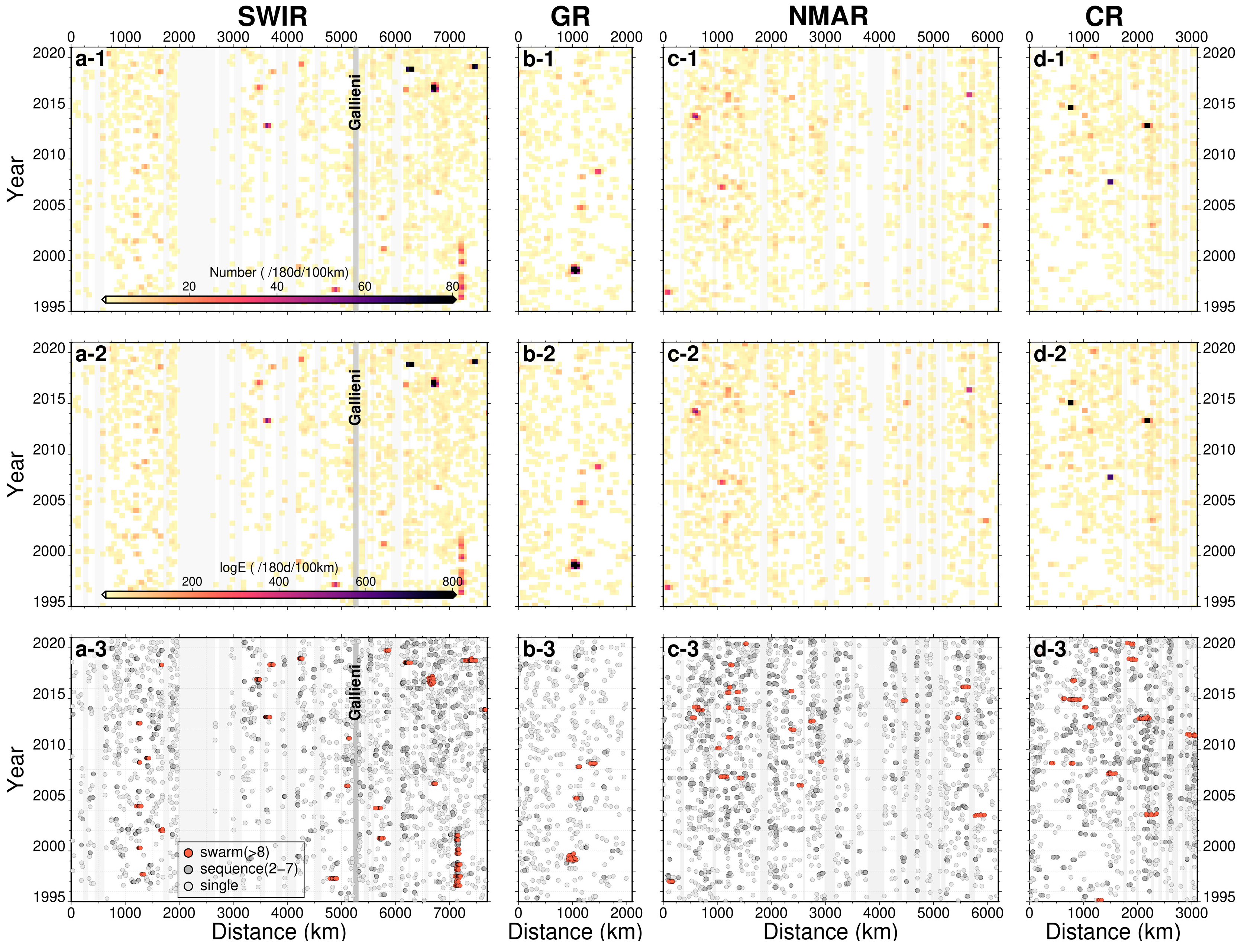
At the SWIR, we identified 34 seismic swarms that include 1015 earthquakes (32% of the whole catalog of the SWIR), yielding a swarm-type seismicity rate of (Table 3). Notably, three large seismic swarms occurred to the east of the Gallieni transform fault (Figure 4 and Figure 7), which are SWIR-19 (192 events during 20 days at the SWIR 58° E), SWIR-20 (211 events during 310 days at SWIR 61° E), and SWIR-33 (88 events during 79 days at SWIR 67° E). For the events with of these three swarms, the focal mechanisms, based on the Global Centroid-Moment-Tensor (www.globalcmt.org, accessed on 15 March 2024), indicate normal faulting on ridge-parallel planes (Figure 4). The non-swarm-type earthquakes are 819 (25% for sequence) and 1387 (43% for single) events, with a seismicity rate of (Table 3). To the east of the Gallieni transform fault, both seismicity rates of swarm-type and non-swarm-type earthquakes are higher ( and , respectively) than those to the west ( and , respectively).
At the GR, we identified 4 seismic swarms that include 249 earthquakes (31% of the whole catalog of the GR), yielding a swarm-type seismicity rate of (Table 3). A notable large seismic swarm occurred at 85° E in 1999 (GR-1 with 198 events over 250 days). Additionally, only three small seismic swarms occurred, and no swarm was observed in the past 10 years (Figure 5). The non-swarm-type earthquakes are 110 (14% for sequence) and 441 (55% for single) events, with a seismicity rate of (Table 3).
At the NMAR, we identified 24 seismic swarms that include 404 earthquakes (16% of the whole catalog of the NMAR), yielding a swarm-type seismicity rate of (Table 3). The largest seismic swarm has 48 events over 12 days (NMAR-23). The non-swarm-type earthquakes are 1029 (40% for sequence) and 1141 (44% for single) events with a seismicity rate of (Table 3). These seismic swarms mostly occurred in the north (along-axis distance between 0 and 3000 km), while only four occurred in the south (Figure 5(c-3)).
At the CR, we identified 16 seismic swarms that include 457 earthquakes (27% of the whole catalog of the CR), yielding a swarm-type seismicity rate of (Table 3). The largest seismic swarm recorded 129 events over 74 days (CR-14). The non-swarm-type earthquakes are 634 (38% for sequence) and 574 (35% for single) events with a seismicity rate of (Table 3).
4. Discussion
Our analysis of the teleseismic catalog at slow–ultraslow-spreading ridges reveals three distinct patterns of seismicity: seismic swarm, sequence, and single. This allows us to systematically explore the relationship between seismic swarm and volcanic activity, and investigate how the spreading rate and the regional melt supply influence the pattern of seismicity.
4.1. Seismic Swarms Indicate Volcanic Activity
Seismic swarms are considered to be primarily triggered by physical processes, such as fluid flow in the lithosphere and shear slip in non-seismic zones; therefore, they are generally no obvious mainshock–aftershock pattern [6]. Seismic swarms of volcanic origin typically involve fluids, and their spatiotemporal evolution in seismic activity aligns with magmatic activity, as observed in Iceland [32,33,34]. In our study areas, the most typical example is the seismic swarm that occurred in the GR at 85° E in 1999 (GR-1, Figure 7 and Figure 8b). This seismic swarm consisted of 198 events occurring within 250 days, with all magnitudes over 4 (the average magnitude is 4.5, and the maximum magnitude is 5.4). The nearby fresh pyroclastic deposits confirmed that this seismic swarm was accompanied by a volcanic eruption that built a significant submarine volcano [35]. We propose that other seismic swarms occurring in the study area may also relate to volcanic activity, supported by the following reasons:
- The duration of seismic swarms ranges from several days to several weeks, and the seismicity rate during the period of seismic swarms is much higher than that during the period of non-seismic swarms (Figure 9). For example, in 2018, two large seismic swarms (SWIR-19 and SWIR-33) occurred in the eastern part of SWIR (Figure 8a), and there were 192 (the average magnitude is 4.6 and the maximum magnitude is 5.7) and 88 (the average magnitude is 4.6 and the maximum magnitude is 5.7) events recorded, respectively. Notably, these two seismic swarms were also detected by hydrophones; 1109 (SWIR-19) and 4880 (SWIR-33 in Figure 8a) events with smaller magnitudes were recorded over 13 and 33 days, respectively [2].
- All seismic swarms identified in our study area have at least one event with a magnitude over 4.7 (Table 2). McNutt [31] reports that magma intrusions and volcanic eruptions are usually accompanied by seismic swarms with magnitudes of 2–3; earthquakes with magnitudes of 4–5 or higher may occur with a volcanic event.
- Seismic swarms often occurred in proximity to the volcanic center of second-order segments, similar to the finding by [4]. These volcanic segment centers are characterized by a higher melt supply with more volcanic constructions (e.g., Figure 8), relative to their segment ends due to along-axis melt focusing [36,37], probably responsible for the higher likelihood of seismic swarm occurrence. However, not all volcanic centers have seismic swarms between 1995 and 2020, possibly due to the large interval of the volcanic eruptions at slow–ultraslow-spreading ridges (up to thousands of years) [18]. Additionally, we might miss small-magnitude seismic swarms associated with minor volcanic eruptions, as we only consider earthquake magnitudes over 4.
4.2. The Influence of the Spreading Rate
We compare the seismicity rates (number of earthquakes per 100 km) of swarm-type, sequence-type, and single earthquakes of the four studied MORs (Figure 10). The swarm-type seismicity rates (red circles in Figure 10) at the SWIR (19.6/100 km) and CR (17.9/100 km) are higher than those of the GR and NMAR, as they contain more large seismic swarms (>70 events). The SWIR, CR, and GR have three (SWIR-19, SWIR-20, and SWIR-33), two (CR-4 and CR-14), and one (GR-1) large seismic swarms, respectively, and the NMAR has none. After excluding these large seismic swarms, we recalculate the seismicity rate of the swarm-type earthquakes (pink triangles in Figure 10), resulting in comparable values at the SWIR, NMAR, and CR (~10/100 km) and a low value at the GR (2.5/100 km). We, therefore, propose that ultraslow-spreading ridges have a higher possibility to generate large seismic swarms than slow-spreading ridges, probably relating to thicker axial lithospheres [19] and an overall higher degree of along-axis melt focusing [40]. In addition, the seismicity rates of sequence-type earthquakes increase with the spreading rate (dark gray circles in Figure 10), probably due to that the frequency of small-scale volcanic activities that produce earthquakes with magnitudes mostly less than 4 is increasing with the spreading rate. The resulting small seismic swarms are defined as sequences or blind in our study.
4.3. The Influence of the Regional Melt Supply
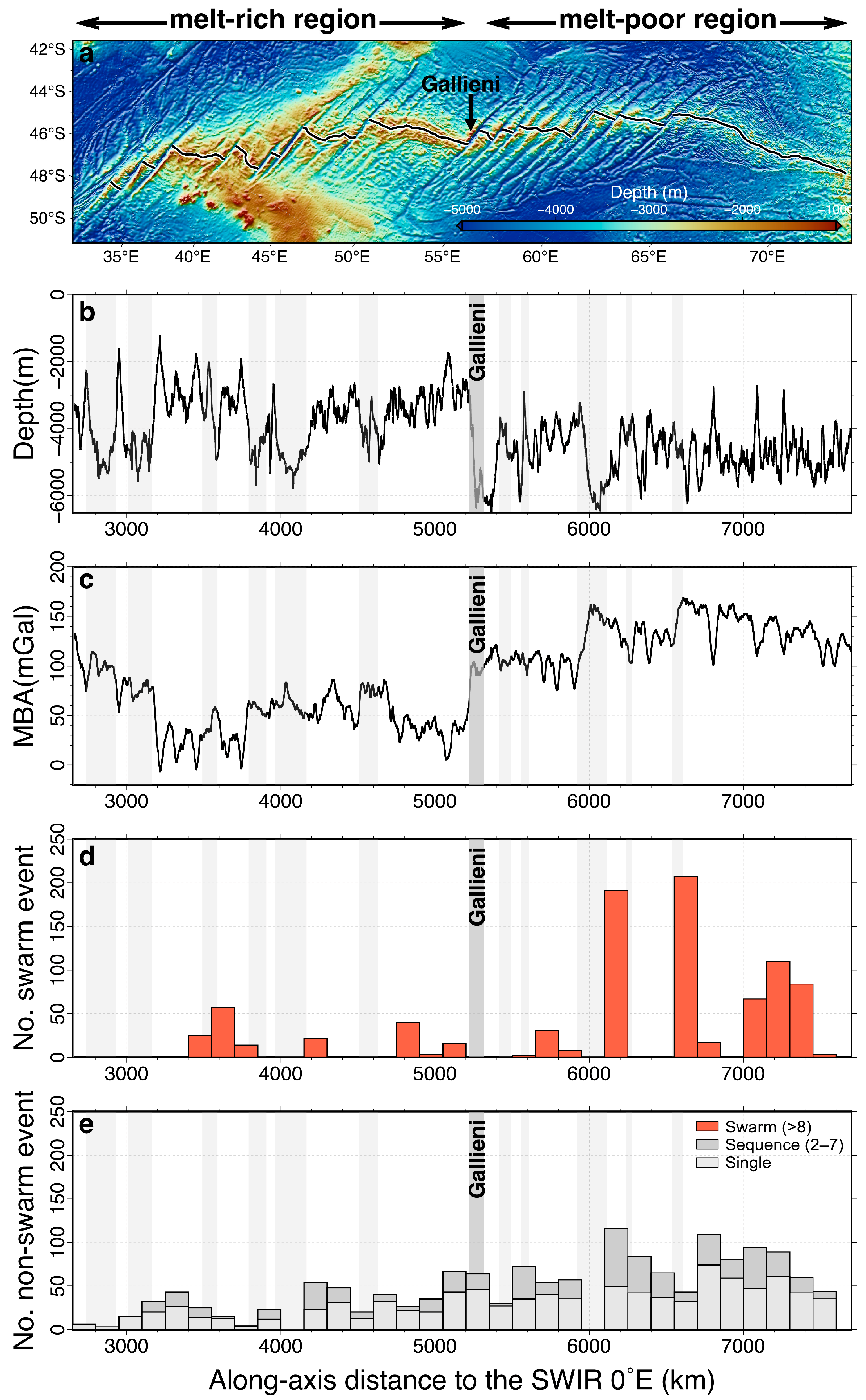
To explore the influence of the melt supply on the seismicity, we compare two regions with the most contrasting melt supply at the ultraslow-spreading SWIR, according to the variations in axial topography and the mantle Bouguer gravity anomaly (MBA) (Figure 9) [38,39,41]. These two regions are the melt-poor eastern region (SWIR 32–52.5° E at along-axis distance between 2650 and 5200 km) and the melt-rich central region (SWIR 52.5–70° E at along-axis distance between 5250 and 7700 km). The melt-poor eastern SWIR corresponds to a topographic low, an MBA high, a detachment-faulting-dominated seafloor morphology, and a relatively low heat flow, while the melt-rich central SWIR corresponds to a topographic high, an MBA low, a volcanic-dominated seafloor morphology, and a slightly high heat flow (Figure 9a–c and Figure S3) [14,39,41,42]. We find that both swarm-type and non-swarm-type earthquakes exhibit higher seismicity rates in the melt-poor eastern SWIR (Figure 9d,e). This finding could be explained by an overall colder and thicker lithosphere with a higher degree of along-axis melt focusing to segment centers at the eastern SWIR, relative to the central SWIR [14,40], which may also be responsible for the large seismic swarms at the eastern SWIR (e.g., SWIR-19, 20, and 33). This relationship may be also applicable to slow-spreading ridges. For example, the seismic swarms in NMAR primarily focus on the region of 15–30° E (along-axis distance between 1000 and 3000 km) (Figure 5(c-3)), corresponding to a relative low melt supply with a topographic low and an MBA high morphology [43].
5. Conclusions
ISC teleseismic data between 1995 and 2020 along the ultraslow-spreading SWIR and GR and the slow-spreading NMAR and CR have been systematically analyzed and shown to have a highly spatiotemporal variation. A total of 78 seismic swarms (each contains ≥8 earthquakes, and 80% occur within 20 days), 877 sequences, and 3543 single events were identified. Most of the seismic swarms occurred near the volcanic centers of the second-order ridge segments, serving as indicators of volcanic activity at these ridges. We also find that ultraslow-spreading ridges, relative to slow-spreading ridges, have a higher potential to produce large seismic swarms that contain >70 events (e.g., SWIR-19, 20, GR-1). While slow-spreading ridges likely exhibit seismic sequences, probably attributed to high-frequency small-scale melt intrusions that produce earthquakes with magnitudes mostly less than 4. Moreover, at ultraslow-spreading ridges, the seismicity rates of both swarm-type and non-swarm-type earthquakes are higher at the melt-poor eastern SWIR than those at the melt-rich central SWIR. We, therefore, propose that as the spreading rate and the melt supply decrease at slow–ultraslow-spreading ridges, the lithosphere becomes colder and thicker with a higher degree of along-axis melt focusing (the most extreme example at the eastern SWIR), which results in a higher seismicity rate and a higher possibility of large volcano-induced seismic swarms.
Supplementary Materials
The following supporting information can be downloaded at: https://www.mdpi.com/article/10.3390/jmse12040605/s1, Figure S1: Different search radii on earthquake density; Figure S2: Different search radii on earthquake moment release intensity; Figure S3: Heat flow [42] along the SWIR axis at distance between 2650 and 7000 km (SWIR 32–70° E).
Author Contributions
Conceptualization, K.Y. and J.C.; methodology, K.Y. and J.C.; software, K.Y.; validation, K.Y., J.C. and T.Z.; formal analysis, K.Y., J.C. and T.Z.; investigation, K.Y. and J.C.; resources, K.Y. and J.C.; data curation, K.Y.; writing—original draft preparation, K.Y.; writing—review and editing, K.Y., J.C. and T.Z.; visualization, K.Y. and J.C.; supervision, J.C. and T.Z.; project administration, T.Z.; funding acquisition, T.Z. All authors have read and agreed to the published version of the manuscript.
Funding
This research was supported by Science Foundation of Donghai Laboratory under Grant No. DH-2022ZY0007; the Natural Science Foundation of China under Grant No. 42176086 and 42206066; And Zhejiang Provincial Natural Science Foundation of China under Grant No. LDQ23D060001.
Institutional Review Board Statement
Not applicable.
Informed Consent Statement
Not applicable.
Data Availability Statement
The original data presented in the study are openly available in www.isc.ac.uk.
Acknowledgments
All figures in this paper were created using GMT [44]. All seismic data in this paper were provided by the International Seismological Centre (ISC).
Conflicts of Interest
The authors declare no conflict of interest.
References
- Chen, J.; Crawford, W.C.; Cannat, M. Microseismicity and lithosphere thickness at a nearly-amagmatic oceanic detachment fault system. Nat. Commun. 2023, 14, 430. [Google Scholar] [CrossRef] [PubMed]
- Ingale, V.V.; Bazin, S.; Royer, J.-Y. Hydroacoustic Observations of Two Contrasted Seismic Swarms along the Southwest Indian Ridge in 2018. Geosciences 2021, 11, 225. [Google Scholar] [CrossRef]
- Parnell-Turner, R.; Smith, D.K.; Dziak, R.P. Hydroacoustic Monitoring of Seafloor Spreading and Transform Faulting in the Equatorial Atlantic Ocean. J. Geophys. Res. Solid Earth 2022, 127, e2022JB024008. [Google Scholar] [CrossRef]
- Schlindwein, V. Teleseismic earthquake swarms at ultraslow spreading ridges: Indicator for dyke intrusions? Geophys. J. Int. 2012, 190, 442–456. [Google Scholar] [CrossRef]
- Tolstoy, M.; Bohnenstiehl, D.R.; Edwards, M.H.; Kurras, G.J. Seismic character of volcanic activity at the ultraslow-spreading Gakkel Ridge. Geology 2001, 29, 1139–1142. [Google Scholar] [CrossRef]
- Chen, X.; Shearer, P.M.; Abercrombie, R.E. Spatial migration of earthquakes within seismic clusters in Southern California: Evidence for fluid diffusion. J. Geophys. Res. Solid Earth 2012, 117. [Google Scholar] [CrossRef]
- Korger, E. The Volcanic Earthquake Swarm of 1999 at the Eastern Gakkel Ridge, Arctic Ocean: A Case Study for a Comparison between a Probabilistic- and a Conventional Teleseismic Algorithm. 2010. Available online: https://epic.awi.de/id/eprint/23458/ (accessed on 21 March 2024).
- Escartín, J.; Smith, D.K.; Cann, J.R.; Schouten, H.; Langmuir, C.H.; Escrig, S. Central role of detachment faults in accretion of slow-spreading oceanic lithosphere. Nature 2008, 455, 790–794. [Google Scholar] [CrossRef]
- Phipps Morgan, J.; Chen, Y.J. Dependence of ridge-axis morphology on magma supply and spreading rate. Nature 1993, 364, 706–708. [Google Scholar] [CrossRef]
- Chen, J.; Olive, J.A.; Cannat, M. Beyond spreading rate: Controls on the thermal regime of mid-ocean ridges. Proc. Natl. Acad. Sci. USA 2023, 120, e2306466120. [Google Scholar] [CrossRef]
- Chen, J.; Olive, J.-A.; Cannat, M. Thermal Regime of Slow and Ultraslow Spreading Ridges Controlled by Melt Supply and Modes of Emplacement. J. Geophys. Res. Solid Earth 2022, 127, e2021JB023715. [Google Scholar] [CrossRef]
- Rundquist, D.V.; Sobolev, P.O. Seismicity of mid-oceanic ridges and its geodynamic implications: A review. Earth-Sci. Rev. 2002, 58, 143–161. [Google Scholar] [CrossRef]
- Cannat, M.; Sauter, D.; Lavier, L.; Bickert, M.; Momoh, E.; Leroy, S. On spreading modes and magma supply at slow and ultraslow mid-ocean ridges. Earth Planet. Sci. Lett. 2019, 519, 223–233. [Google Scholar] [CrossRef]
- Chen, J.; Zhang, T.; Li, H.; Tao, C.; Cannat, M.; Sauter, D. Evolution of enhanced magmatism at the ultraslow spreading Southwest Indian Ridge between 46°E and 53.5°E. Tectonophysics 2023, 860, 229903. [Google Scholar] [CrossRef]
- Dick, H.J.B.; Lin, J.; Schouten, H. An ultraslow-spreading class of ocean ridge. Nature 2003, 426, 405–412. [Google Scholar] [CrossRef] [PubMed]
- Minshull, T.A.; Muller, M.R.; White, R.S. Crustal structure of the Southwest Indian Ridge at 66°E: Seismic constraints. Geophys. J. Int. 2006, 166, 135–147. [Google Scholar] [CrossRef]
- Sauter, D.; Cannat, M.; Rouméjon, S.; Andreani, M.; Birot, D.; Bronner, A.; Brunelli, D.; Carlut, J.; Delacour, A.; Guyader, V.; et al. Continuous exhumation of mantle-derived rocks at the Southwest Indian Ridge for 11 million years. Nat. Geosci. 2013, 6, 314–320. [Google Scholar] [CrossRef]
- Perfit, M.R.; Chadwick, W.W., Jr. Magmatism at Mid-Ocean Ridges: Constraints from Volcanological and Geochemical Investigations. In Faulting and Magmatism at Mid-Ocean Ridges; American Geophysical Union: Washington, DC, USA, 1998; pp. 59–115. [Google Scholar]
- Grevemeyer, I.; Hayman, N.W.; Lange, D.; Peirce, C.; Papenberg, C.; Van Avendonk, H.J.A.; Schmid, F.; de La Peña, L.G.; Dannowski, A. Constraining the maximum depth of brittle deformation at slow- and ultraslow-spreading ridges using microseismicity. Geology 2019, 47, 1069–1073. [Google Scholar] [CrossRef]
- Yu, Z.; Li, J.; Niu, X.; Rawlinson, N.; Ruan, A.; Wang, W.; Hu, H.; Wei, X.; Zhang, J.; Liang, Y. Lithospheric Structure and Tectonic Processes Constrained by Microearthquake Activity at the Central Ultraslow-Spreading Southwest Indian Ridge (49.2° to 50.8°E). J. Geophys. Res. Solid Earth 2018, 123, 6247–6262. [Google Scholar] [CrossRef]
- Heyburn, R.; Bowers, D.; Green, D.N. Seismic and hydroacoustic observations from recent underwater events in the South Atlantic Ocean. Geophys. J. Int. 2020, 223, 289–300. [Google Scholar] [CrossRef]
- Smets, P.S.M.; Weemstra, K.; Evers, L.G. Long-Range Hydroacoustic Observations of the Monowai Volcanic Centre as a Proxy for Seasonal Variations in Sound Propagation. In Proceedings of the EGU General Assembly 2020, Online, 4–8 May 2020. EGU2020-18440. [Google Scholar] [CrossRef]
- Tepp, G.; Dziak, R.P.; Haney, M.M.; Lyons, J.J.; Searcy, C.; Matsumoto, H.; Haxel, J. Seismic and hydroacoustic observations of the 2016–17 Bogoslof eruption. Bull. Volcanol. 2019, 82, 4. [Google Scholar] [CrossRef]
- Bergman, E.A.; Solomon, S.C. Earthquake swarms on the Mid-Atlantic Ridge: Products of magmatism or extensional tectonics? J. Geophys. Res. Solid Earth 1990, 95, 4943–4965. [Google Scholar] [CrossRef]
- Frohlich, C.; Davis, S.D. Single-Link Cluster Analysis as a Method to Evaluate Spatial and Temporal Properties of Earthquake Catalogues. Geophys. J. Int. 1990, 100, 19–32. [Google Scholar] [CrossRef]
- Chen, J.; Zhang, T.; Tominaga, M.; Escartin, J.; Kang, R. Ocean Sciences with the Spilhaus Projection: A Seamless Ocean Map for Spatial Data Recognition. Sci. Data 2023, 10, 410. [Google Scholar] [CrossRef] [PubMed]
- Scordilis, E.M. Empirical Global Relations Converting MS and mb to Moment Magnitude. J. Seismol. 2006, 10, 225–236. [Google Scholar] [CrossRef]
- Kanamori, H. The energy release in great earthquakes. J. Geophys. Res. (1896–1977) 1977, 82, 2981–2987. [Google Scholar] [CrossRef]
- Davis, S.D.; Frohlich, C. Single-link cluster analysis, synthetic earthquake catalogues, and aftershock identification. Geophys. J. Int. 1991, 104, 289–306. [Google Scholar] [CrossRef]
- Mogi, K. Some Discussions on Aftershocks, Foreshocks and Earthquake Swarms: The Fracture of a Semi-infinite Body Caused by an Inner Stress Origin and Its Relation to the Earthquake Phenomena, 3rd ed.; Earthquake Research Institute, University of Tokyo: Tokyo, Japan, 1963; pp. 615–658. [Google Scholar]
- McNutt, S.R. Seismic Monitoring and Eruption Forecasting of Volcanoes: A Review of the State-of-the-Art and Case Histories. In Monitoring and Mitigation of Volcano Hazards; Springer: Berlin/Heidelberg, Germany, 1996; pp. 99–146. [Google Scholar]
- Einarsson, P. Seismicity and earthquake focal mechanisms along the Mid-Atlantic plate boundary between Iceland and the Azores. Tectonophysics 1979, 55, 127–153. [Google Scholar] [CrossRef]
- Hough, S.E.; Dollar, R.S.; Johnson, P. The 1998 Earthquake Sequence South of Long Valley Caldera, California: Hints of Magmatic Involvement. Bull. Seismol. Soc. Am. 2000, 90, 752–763. [Google Scholar] [CrossRef]
- Yukutake, Y.; Ito, H.; Honda, R.; Harada, M.; Tanada, T.; Yoshida, A. Fluid-induced swarm earthquake sequence revealed by precisely determined hypocenters and focal mechanisms in the 2009 activity at Hakone volcano, Japan. J. Geophys. Res. Solid Earth 2011, 116. [Google Scholar] [CrossRef]
- Sohn, R.A.; Willis, C.; Humphris, S.; Shank, T.M.; Singh, H.; Edmonds, H.N.; Kunz, C.; Hedman, U.; Helmke, E.; Jakuba, M.; et al. Explosive volcanism on the ultraslow-spreading Gakkel ridge, Arctic Ocean. Nature 2008, 453, 1236–1238. [Google Scholar] [CrossRef]
- Cannat, M.; Rommevaux-Jestin, C.; Fujimoto, H. Melt supply variations to a magma-poor ultra-slow spreading ridge (Southwest Indian Ridge 61° to 69°E). Geochem. Geophys. Geosystems 2003, 4. [Google Scholar] [CrossRef]
- Lin, J.; Purdy, G.M.; Schouten, H.; Sempere, J.C.; Zervas, C. Evidence from gravity data for focusedmagmatic accretionalong the Mid-Atlantic Ridge. Nature 1990, 344, 627–632. [Google Scholar] [CrossRef]
- Georgen, J.E.; Lin, J.; Dick, H.J.B. Evidence from gravity anomalies for interactions of the Marion and Bouvet hotspots with the Southwest Indian Ridge: Effects of transform offsets. Earth Planet. Sci. Lett. 2001, 187, 283–300. [Google Scholar] [CrossRef]
- Sauter, D.; Cannat, M. The Ultraslow Spreading Southwest Indian Ridge. In Diversity of Hydrothermal Systems on Slow Spreading Ocean Ridges; American Geophysical: Union Washington, DC, USA, 2010; pp. 153–173. [Google Scholar]
- Cannat, M.; Rommevaux-Jestin, C.; Sauter, D.; Deplus, C.; Mendel, V. Formation of the axial relief at the very slow spreading Southwest Indian Ridge (49° to 69°E). J. Geophys. Res. Solid Earth 1999, 104, 22825–22843. [Google Scholar] [CrossRef]
- Zhang, T.; Lin, J.; Gao, J. Magmatism and tectonic processes in Area A hydrothermal vent on the Southwest Indian Ridge. Sci. China Earth Sci. 2013, 56, 2186–2197. [Google Scholar] [CrossRef]
- Lucazeau, F. Analysis and Mapping of an Updated Terrestrial Heat Flow Data Set. Geochem. Geophys. Geosystems 2019, 20, 4001–4024. [Google Scholar] [CrossRef]
- Thibaud, R.; Gente, P.; Maia, M. A systematic analysis of the Mid-Atlantic Ridge morphology and gravity between 15°N and 40°N: Constraints of the thermal structure. J. Geophys. Res. Solid Earth 1998, 103, 24223–24243. [Google Scholar] [CrossRef]
- Wessel, P.; Smith, W.H.F. New version of the generic mapping tools. Eos Trans. Am. Geophys. Union 1995, 76, 329. [Google Scholar] [CrossRef]
Figure 1.
Bathymetric map and teleseismic distribution of the study area. (a) Spilhaus global map [26]. The pink dots represent the distribution of global teleseismic locations with magnitudes ≥ 3 between 1990 and 2020. The earthquake catalog is sourced from the International Seismic Center (ISC, www.isc.ac.uk, accessed on 5 March 2022); the red dots represent the distribution of teleseismic events in the study area. (b–e) Bathymetric maps of the ultraslow-spreading Southwest Indian Ridge (SWIR) and Gakkel Ridge (GR), and the slow-spreading North Mid-Atlantic Ridge (NMAR) and the Carlsberg Ridge (CR). The distance scales of the four MORs are the same. The earthquakes are drawn with color-coded magnitude ranges: magnitude 3–4 (blue), 4–4.5 (yellow), 4.5–5 (orange), and 5 and above (red). (f) Pie chart of the seismic magnitudes for the four MORs.

Figure 2.
Completeness magnitude (Mc) analysis. The gray dots represent the cumulative number of earthquakes on the four MORs; the Mc of the whole selected earthquake catalog is 4.3 (red dot); the pink, yellow, blue, and green dots represent the cumulative numbers of earthquakes on the SWIR, GR, NMAR, and CR, respectively, with Mc of 4.2, 4.0, 4.1, and 4.1 (red dots).

Figure 3.
Spatiotemporal variations in teleseismicity. The distance scales of the four ridges are the same. The westernmost points of the SWIR and GR are defined as the starting point (distance = 0), and the northernmost points of the NMAR and CR are defined as the starting point. (a-1–a-4) Spatiotemporal analysis of the SWIR teleseismicity. (a-1) Magnitude pie chart. Yellow represents 4–4.5, orange represents 4.5–5, and red represents over 5. (a-2) Histogram of along-axis distribution, binned at 100 km. (a-3) Histogram of time distribution, binned at 1 year. The blue line represents 1995. (a-4) Scatter plot of spatiotemporal distribution. (b-1–b-4) GR teleseismicity. (c-1–c-4) NMAR teleseismicity. (d-1–d-4) CR teleseismicity.

Figure 4.
Illustration of seismic cluster. (a) Bathymetric map of the SWIR from 58° E to 70° E at along-axis distance between 6000 and 7000 km. The dots on the map indicate the locations of earthquakes that occurred during 2016–2020. The white dots represent non-swarm-type earthquakes, and swarm-type earthquakes are divided using magnitudes indicated by colored dots (yellow: magnitude 4–4.5, orange: magnitude 4.5–5, red: magnitude > 5). Focal mechanisms are shown for 52 large events () of 3 swarms (SWIR-19, SWIR-20, SWIR-33). (b) Scatter plot of the spatiotemporal distribution of the original earthquakes. (c) Scatter plot of the spatiotemporal distribution of earthquakes. Seismic swarms with 8 or more earthquakes (red) are selected by single-link cluster analysis. Dark gray represents clusters with 2–7 earthquakes (sequences), and light gray represents single earthquakes. (d) Earthquake number density map. (e) Moment release intensity map.

Figure 5.
Seismic clusters selection results of four MORs. The distances, respectively, represent the along-axis distance to the SWIR 0° E, the GR 6° E, the NMAR 35° N and the CR 10° N. (a-1,b-1,c-1,d-1) Earthquake number density; (a-2,b-2,c-2,d-2) Seismic moment release intensity; (a-3,b-3,c-3,d-3) Spatiotemporal distribution scatter plots of seismic clusters. The light gray areas represent transform faults, and the Gallieni transform fault of the SWIR specifically is denoted in dark gray.

Figure 6.
Histogram of seismic clusters. (a) Histogram of all seismic clusters of the four MORs, with a pie chart representing the proportions of different types of earthquakes. (b–e) SWIR, GR, NMAR, and CR.
Figure 6.
Histogram of seismic clusters. (a) Histogram of all seismic clusters of the four MORs, with a pie chart representing the proportions of different types of earthquakes. (b–e) SWIR, GR, NMAR, and CR.

Figure 7.
Seismic swarm duration. (a,b) Duration of all identified seismic swarms vs. number of earthquakes. (c,d) Duration of seismic swarms vs. their cumulative moment release. See legend for seismic swarms in (a) at different ridges.
Figure 7.
Seismic swarm duration. (a,b) Duration of all identified seismic swarms vs. number of earthquakes. (c,d) Duration of seismic swarms vs. their cumulative moment release. See legend for seismic swarms in (a) at different ridges.

Figure 8.
Three typical seismic swarms (SWIR-33, GR-1, and SWIR-30). (a) Bathymetric map showing spatiotemporal distribution of the seismic swarm SWIR-33. White dots represent earthquake locations by hydrophone data [2]. Focal mechanisms are shown for large events (). Yellow dots represents 4–4.5, orange represents 4.5–5, and red represents over 5. (b) Bathymetric map showing spatiotemporal distribution of the seismic swarm GR-1. (c) Bathymetric map showing spatiotemporal distribution of the seismic swarm SWIR-30.

Figure 9.
Along-axis profile of the SWIR 32–70° E at along-axis distance between 2650 and 7000 km. (a) Bathymetric maps of the SWIR 32–70° E. Black line represents the location of the ridge axis. (b,c) Depth and Bouguer gravity anomaly (MBA) profile [38,39]. The gray areas represent the locations of transform faults. The Gallieni transform fault is highlighted, which is the boundary of the eastern melt-poor and central melt-rich regions. (d,e) Histogram of swarm-type and non-swarm-type earthquakes, respectively, binned at 150 km.

Figure 10.
Seismicity rate of three types of earthquakes vs. the spreading rate. The red dots represent the seismicity rate of swarm-type earthquakes. The light red triangles represent the seismicity rate of swarm-type earthquakes with <70 events. The orange and gray dots represent sequence-type and single earthquakes, respectively.


Table 1.
Post-1995 earthquakes with magnitudes over 4.
| Ultraslow-Spreading Ridge | Slow-Spreading Ridge | |||||
|---|---|---|---|---|---|---|
| SWIR | GR | Total | NMAR | CR | Total | |
| Spreading rate () | 14–16 | 6–12 | — | 21–27 | 22–26 | — |
| Length (km) | 5200 | 2050 | 7250 | 4500 | 2550 | 7050 |
| Number of earthquakes () | 3221 | 800 | 4021 | 2574 | 1665 | 4239 |
| Mean magnitude (Mu) | 4.6 | 4.5 | 4.6 | 4.6 | 4.6 | 4.6 |
| Average seismic moment released () | ||||||
| Seismicity rate () | 2.48 | 1.56 | 2.22 | 2.29 | 2.61 | 2.41 |
| Seismic strain rate ( ) | 7.06 | 4.46 | 6.33 | 6.55 | 6.50 | 6.53 |
Table 2.
Seismic swarm with over 20 events.
| No. | Central Longtitude (°E) | Central Latitude (°N) | Along-Axis Distance (km) | No. Events | Start Day | Duration (Days) | Max. Mu | Average Mu |
|---|---|---|---|---|---|---|---|---|
| SWIR-9 | 38.87 | −44.18 | 3471.61 | 25 | 19 November 2016 | 4.0 | 5.4 | 4.8 |
| SWIR-10 | 39.96 | −43.38 | 3637.82 | 55 | 6 March 2013 | 7.5 | 5.3 | 4.6 |
| SWIR-12 | 43.62 | −41.01 | 4243.33 | 22 | 9 December 2018 | 7.1 | 5.4 | 4.6 |
| SWIR-13 | 48.57 | −38.08 | 4865.40 | 43 | 13 April 1997 | 4.4 | 5.4 | 4.6 |
| SWIR-19 | 58.20 | −31.66 | 6219.68 | 192 | 10 July 2018 | 19.6 | 5.7 | 4.6 |
| SWIR-20 | 61.06 | −29.19 | 6657.43 | 211 | 12 May 2016 | 310.2 | 5.9 | 4.6 |
| SWIR-23 | 65.54 | −27.64 | 7146.44 | 27 | 31 July 1996 | 6.9 | 5.8 | 4.8 |
| SWIR-30 | 65.65 | −27.66 | 7157.44 | 33 | 4 July 1997 | 1.9 | 5.1 | 4.5 |
| SWIR-31 | 65.69 | −27.65 | 7160.43 | 28 | 9 February 2000 | 25.6 | 5.6 | 4.6 |
| SWIR-33 | 67.61 | −26.63 | 7393.52 | 88 | 27 September 2018 | 78.9 | 5.7 | 4.6 |
| GR-1 | 83.68 | 85.66 | 996.90 | 198 | 17 January 1999 | 249.7 | 5.5 | 4.5 |
| GR-4 | 114.49 | 83.62 | 1383.52 | 28 | 5 August 2008 | 10.6 | 5.6 | 4.5 |
| NMAR-1 | −37.11 | 34.32 | 140.42 | 36 | 21 December 1996 | 22.7 | 5.5 | 4.6 |
| NMAR-3 | −40.27 | 32.19 | 607.50 | 34 | 27 February 2014 | 11.5 | 5.5 | 4.4 |
| NMAR-4 | −40.56 | 31.77 | 667.68 | 28 | 11 November 2013 | 35.8 | 5.3 | 4.5 |
| NMAR-6 | −43.16 | 29.07 | 1118.37 | 35 | 23 April 2007 | 6.5 | 5.5 | 4.5 |
| NMAR-23 | −32.61 | 4.56 | 5585.07 | 48 | 18 February 2013 | 11.9 | 5.7 | 4.7 |
| NMAR-24 | −31.33 | 3.12 | 5864.82 | 25 | 20 February 2016 | 44.0 | 5.3 | 4.6 |
| CR-4 | 61.32 | 5.69 | 791.94 | 93 | 25 November 2014 | 12.1 | 5.9 | 4.6 |
| CR-11 | 66.34 | 2.65 | 1497.96 | 67 | 4 August 2007 | 45.1 | 5.2 | 4.5 |
| CR-14 | 67.96 | −1.99 | 2126.46 | 129 | 8 January 2013 | 73.2 | 5.2 | 4.5 |
| CR-16 | 68.07 | −7.84 | 3043.94 | 23 | 18 April 2011 | 72.7 | 5.2 | 4.6 |
Table 3.
Seismicity rates of swarm-type and non-swarm-type earthquakes with magnitudes over 4.
| Ultraslow-Spreading Ridge | Slow-Spreading Ridge | |||||
|---|---|---|---|---|---|---|
| SWIR | GR | Total | NMAR | CR | Total | |
| No. swarm-type earthquakes (frequency) | 1015 (32%) | 249 (31%) | 1264 (31%) | 404 (16%) | 457 (27%) | 861 (20%) |
| No. non-swarm-type earthquakes (frequency) | 2206 (68%) | 551 (69%) | 2757 (69%) | 2170 (84%) | 1208 (73%) | 3378 (80%) |
| Seismicity rate of swarm-type () | 0.78 | 0.49 | 0.70 | 0.36 | 0.72 | 0.49 |
| Seismicity rate of non-swarm-type () | 1.70 | 1.08 | 1.52 | 1.93 | 1.89 | 1.92 |
Disclaimer/Publisher’s Note: The statements, opinions and data contained in all publications are solely those of the individual author(s) and contributor(s) and not of MDPI and/or the editor(s). MDPI and/or the editor(s) disclaim responsibility for any injury to people or property resulting from any ideas, methods, instructions or products referred to in the content. |
© 2024 by the authors. Licensee MDPI, Basel, Switzerland. This article is an open access article distributed under the terms and conditions of the Creative Commons Attribution (CC BY) license (https://creativecommons.org/licenses/by/4.0/).
Share and Cite
MDPI and ACS Style
Yan, K.; Chen, J.; Zhang, T. Teleseismic Indication of Magmatic and Tectonic Activities at Slow- and Ultraslow-Spreading Ridges. J. Mar. Sci. Eng. 2024, 12, 605. https://doi.org/10.3390/jmse12040605
AMA Style
Yan K, Chen J, Zhang T. Teleseismic Indication of Magmatic and Tectonic Activities at Slow- and Ultraslow-Spreading Ridges. Journal of Marine Science and Engineering. 2024; 12(4):605. https://doi.org/10.3390/jmse12040605
Chicago/Turabian StyleYan, Kaixuan, Jie Chen, and Tao Zhang. 2024. "Teleseismic Indication of Magmatic and Tectonic Activities at Slow- and Ultraslow-Spreading Ridges" Journal of Marine Science and Engineering 12, no. 4: 605. https://doi.org/10.3390/jmse12040605
Note that from the first issue of 2016, this journal uses article numbers instead of page numbers. See further details here.