CFD Simulation of Ship Seakeeping Performance and Slamming Loads in Bi-Directional Cross Wave


School of Civil Engineering and Transportation, South China University of Technology, Guangzhou 510641, China
*
Author to whom correspondence should be addressed.
J. Mar. Sci. Eng. 2020, 8(5), 312; https://doi.org/10.3390/jmse8050312
Submission received: 10 April 2020
/
Revised: 26 April 2020
/
Accepted: 28 April 2020
/
Published: 29 April 2020
(This article belongs to the Special Issue CFD Simulations of Marine Hydrodynamics)
Abstract
:Accurate prediction of ship seakeeping performance in complex ocean environment is a fundamental requirement for ship design and actual operation in seaways. In this paper, an unsteady Reynolds-averaged Navier–Stokes (RANS) computational fluid dynamics (CFD) solver with overset grid technique was applied to estimate the seakeeping performance of an S175 containership operating in bi-directional cross waves. The cross wave is reproduced by linear superposition of two orthogonal regular waves in a rectangle numerical wave tank. The ship nonlinear motion responses, bow slamming loads, and green water on deck induced by cross wave with different control parameters such as wave length and wave heading angle are systemically analyzed. The results demonstrate that both vertical and transverse motion responses, as well as slamming pressure of ship induced by cross wave, can be quite large, and they are quite different from those in regular wave. Therefore, ship navigational safety when suffering cross waves should be further concerned.
1. Introduction
The majority of existing ship seakeeping investigations are concerned with ship motion behavior in uni-directional or long-crested waves [1]. As a result, a lot of effort, which includes potential flow, computational fluid dynamics (CFD) and model test methods, is being dedicated to predicting ship motions in 2D regular or even irregular waves in the past few decades [2]. However, realistic sea states are multi-directional or short-crested, with wave components propagating in different directions. Therefore, an in-depth understanding of the multi-directional wave interactions with ship is essential in accurate prediction of ship hydrodynamics in realistic sea wave conditions.
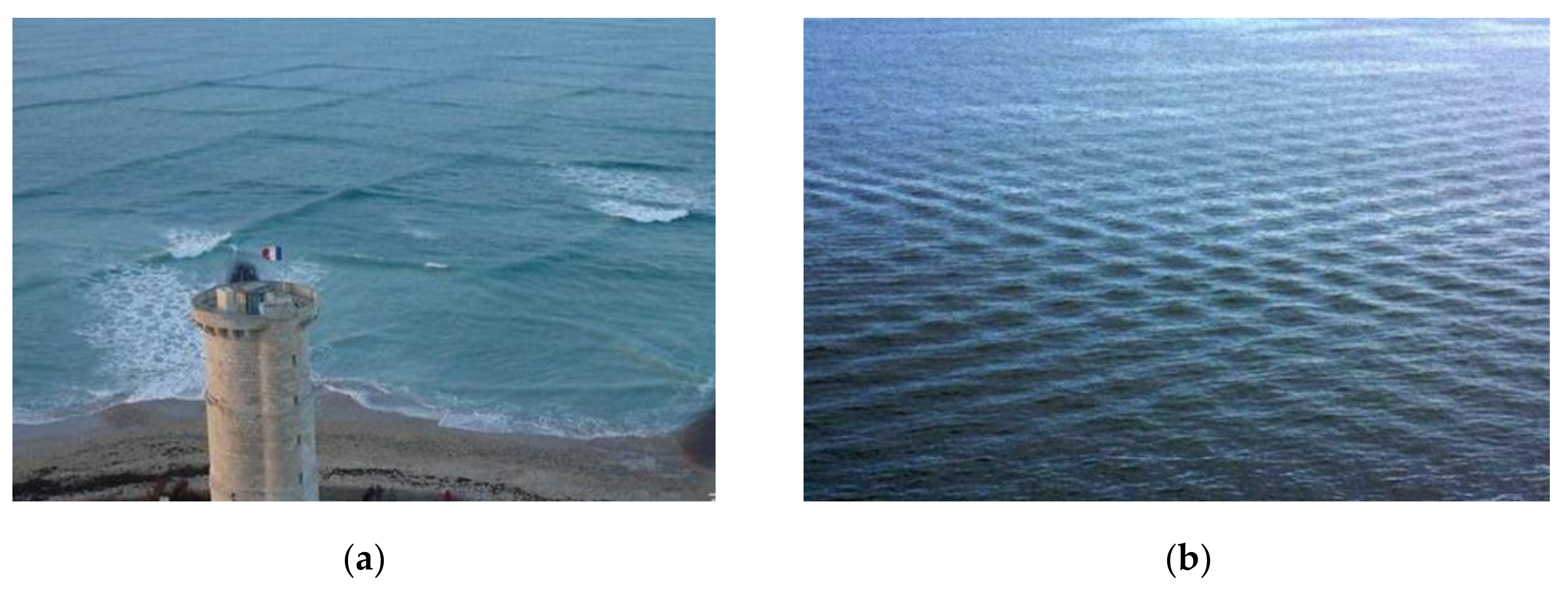
In some places, e.g., the popular tourist destination of the Isle of Rhe, cross wave can be often observed due to the complex and extreme patterns of weather (see Figure 1a). The cross wave can be regarded as the superposition of wind or swell waves coming from two orthogonal directions. An example of the cross wave phenomenon in the ocean is shown in Figure 1. Until now, the problem for the interaction of a ship with a cross wave is not clear and has not been investigated, although people realize that the cross wave may pose a great threat to the safety of the passing ship. Therefore, this paper aims at investigating ship seakeeping behavior in wind-driven bi-directional cross sea waves.
Some researchers have investigated the interaction of multi-directional wave with fixing offshore structures [3,4,5]. However, studies on the seakeeping behavior of free running ships or other floating structures in multi-directional wave are quite limited. Renaud et al. [6] investigated the effect of wave directionality on second-order slow-drift loads and motion response of a Liquefied Natural Gas (LNG) carrier in regular cross waves by a potential flow code and tank model test. Chen et al. [7] numerically investigated ship motions in long-crested and short-crested irregular waves by 3D time domain potential flow theory. Jiao et al. [8] comparatively studied the wave-induced ship motion and load responses in long- and short-crested irregular waves by theoretical and experimental methods. To summarize, the existing investigations on the hydrodynamic behavior of ships in multi-directional waves are mainly conducted by potential flow theory or model experiments, while related investigation by CFD has not been found.
In recent years, CFD, which captures most complexities of the fluid physics with few assumptions, has been widely used as a potential tool in ship design and evaluation [9,10,11]. Although tremendous advances have been made in the CFD simulations of ship motion responses in uni-directional wave [12,13,14], CFD investigations on ship motions induced by multi-directional waves are rarely seen. Recently, fundamental work of multi-directional wave simulation by CFD tool has been conducted by some researchers. For example, Wang et al. [15] simulated 3D directional irregular wave by open-source CFD model REEF3D. Cao and Wan [16] developed a multi-directional nonlinear numerical wave tank by Naoe-FOAM-SJTU solver. Wang et al. [17] calculated the wave forces on a large cylinder in multi-directional irregular waves using a CFD tool. These works focus on the simulation of multi-directional wave and also provide some foundations for the research of ship seakeeping behavior in multi-directional waves using CFD.
This paper focuses on investigating ship seakeeping behavior in bi-directional cross progressive waves by the CFD method, which will also provide some insights into ship motion behavior in multi-directional waves. For this purpose, a cross progressive wave is simulated in a rectangular numerical wave tank, and corresponding ship hydrodynamic behavior are estimated by solving Unsteady Reynolds Averaged Navier–Stokes (URANS) equations. Ship motion response and slamming pressure behavior under different cross wave states are analyzed. This study also provides some useful guidance for the safe operation of a ship when sailing in bi-directional cross seas.
The structure of the rest of this paper is arranged as follows: The description of the adopted S175 containership model, CFD numerical scheme, and calculation conditions are reported in Section 2. In Section 3, the characteristics of a cross wave are analyzed and also demonstrated by CFD simulation results. The seakeeping behavior of a ship in different cross wave conditions are systematically analyzed and discussed in Section 4. The slamming behavior of a ship in typical cross wave conditions is analyzed in Section 5. Finally, the main conclusions and future perspectives are reported in Section 6.
2. Numerical Model Setup
2.1. Ship Model and Geometry
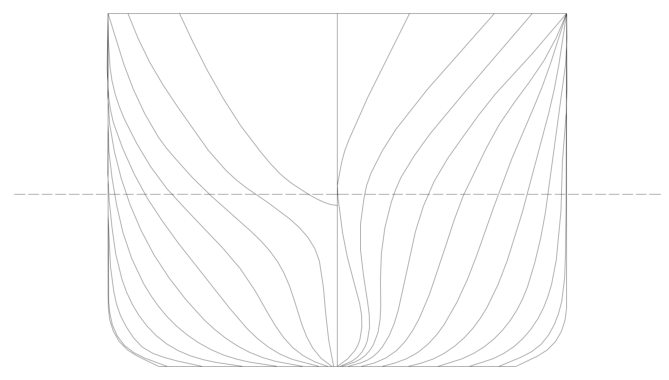
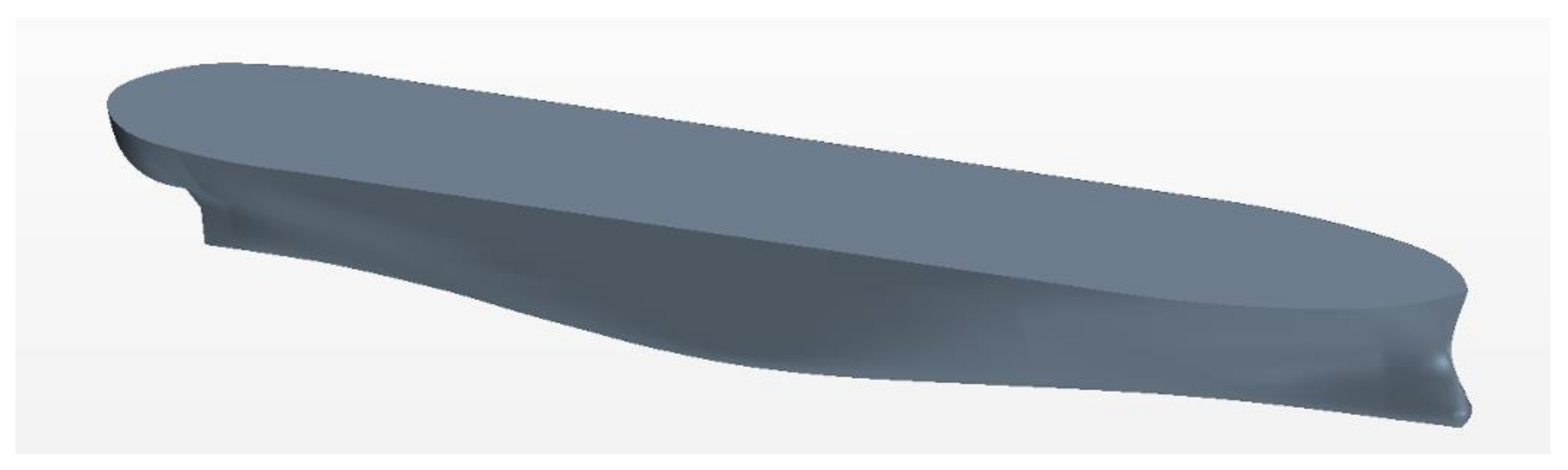
The ship motion simulations in cross wave were applied to a 1:40 scaled S175 containership model without the rudder, propeller, or bilge keels appended. The main particulars of the ship and model are presented in Table 1. Body plan of the ship is shown in Figure 2. A 3D view of the ship hull modeled using STAR-CCM+ software’s pre-processing module is shown in Figure 3.
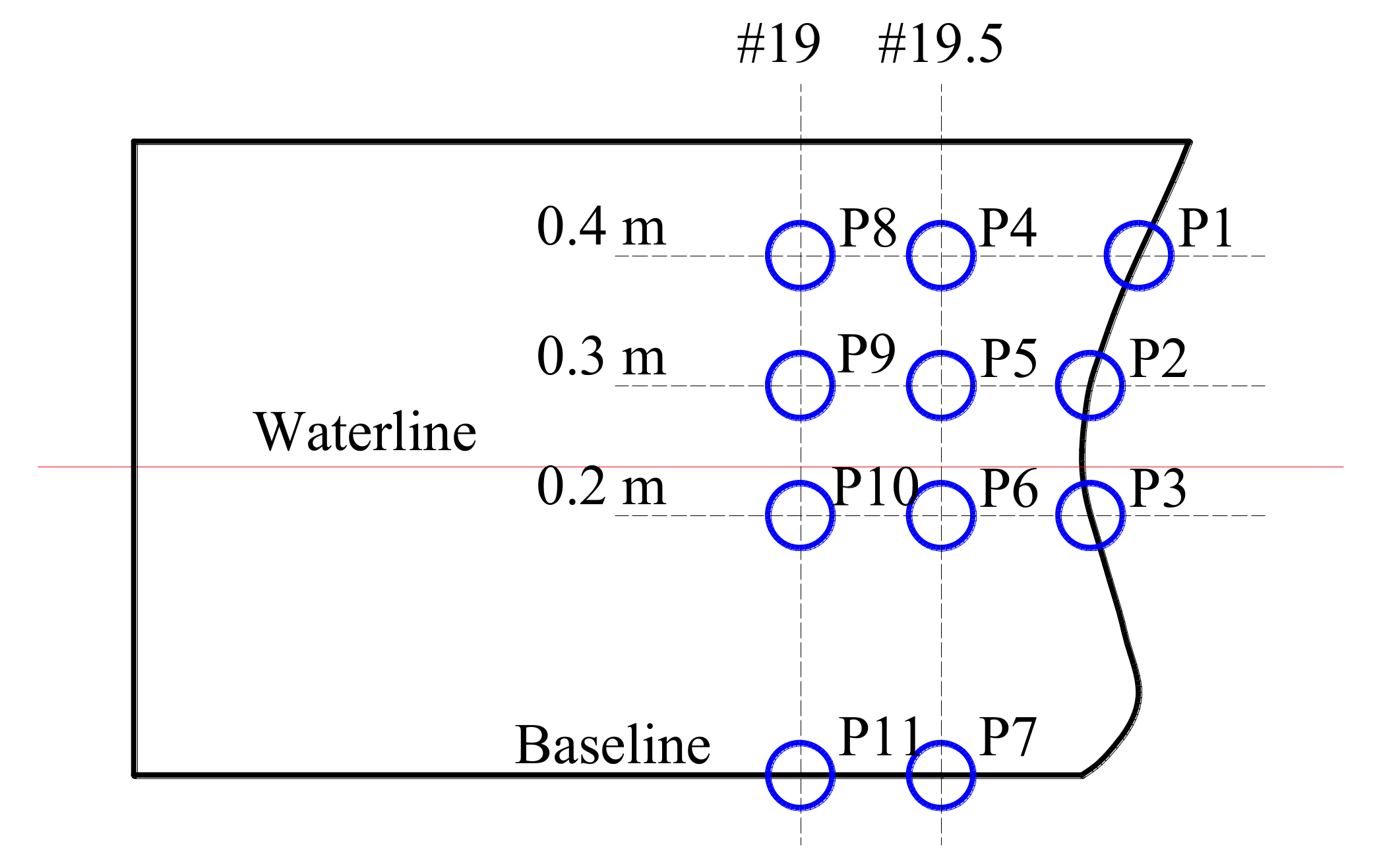
For the investigation of asymmetric impact loads on a ship when sailing in cross waves, an array of 17 pressure sensors were arranged on both the port and starboard sides of the ship bow area. The exact location of the pressure sensors is depicted in Figure 4. The gauges are positioned in the vertical level of baseline, 0.2 m, 0.3 m, or 0.4 m waterline. P1–P3 are located at the centerline of front bow from top to bottom. P4–P7 (or P8–P11) are located at the intersection of cross-section at 19.5th station (or 19th station) with the 0.4 m, 0.3 m, 0.2 m waterline, and the keel. Note that the P4–P6 and P8–P10 exist in both the port and starboard sides of ship, while the P7 and P11 singly locate on the centerline of bow bottom.
2.2. Numerical Scheme
The CFD numerical calculations were performed by the finite volume method (FVM) based STAR-CCM+ software, which use the URANS and Volume of Fluid (VOF) model. The realizable k-ε turbulence model, which provides a good compromise between robustness, computational cost, and accuracy, was used in this study [18,19]. The realizable k-ε turbulence model has more advantages in the simulation of separation flow and flow with larger streamline curvature, which is helpful for the simulation of the flow around hull. A second-order convection scheme was used throughout all simulations to accurately capture sharp interfaces between the two phases of air and water. Convection terms in the RANS formulae were discretised by applying a second-order upwind scheme. The overall solution procedure was obtained according to a SIMPLE-type algorithm. The rigid ship model was free to move in three degrees of freedom (3-DoF), i.e., heave, pitch, and roll, which is realized by the dynamic fluid body interaction (DFBI) model. The motion at ship’s center of gravity (CoG) was monitored and used for analysis.
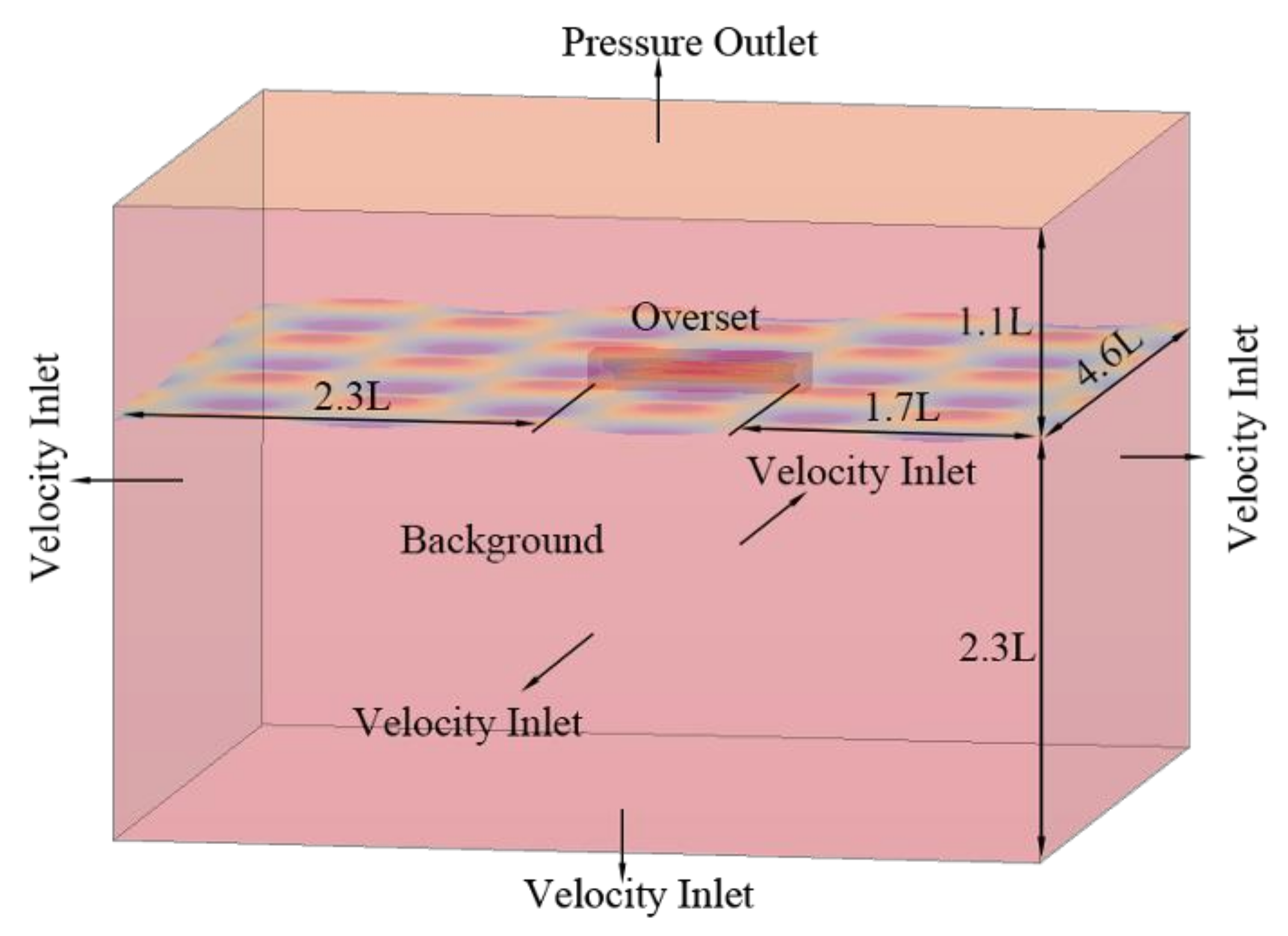
The origin of the coordinate system is located at the intersection of the free surface of calm water, symmetry plane, and cross section at the after perpendicular of the ship. The positive of ox, oy, and oz axes point to the bow, port side, and sky, respectively. A numerical wave tank for the entire fluid domain without symmetry plane was established to simulate the fluid flow. The extents of the computational domain are −2.3 L < x < 2.7 L, −2.3 L < y < 2.3 L, and −2.3 L < z < 1.1 L. For the generation of a multi-directional wave, the boundary conditions of the numerical wave tank were set in the following style: the four sidewalls and bottom of the fluid domain were set as the velocity inlet boundary; the top of the fluid domain was set as the pressure outlet; and the hull body surface was set as the no-slip wall. General view of the fluid domain and the ship model and the notations of boundary conditions are shown in Figure 5.
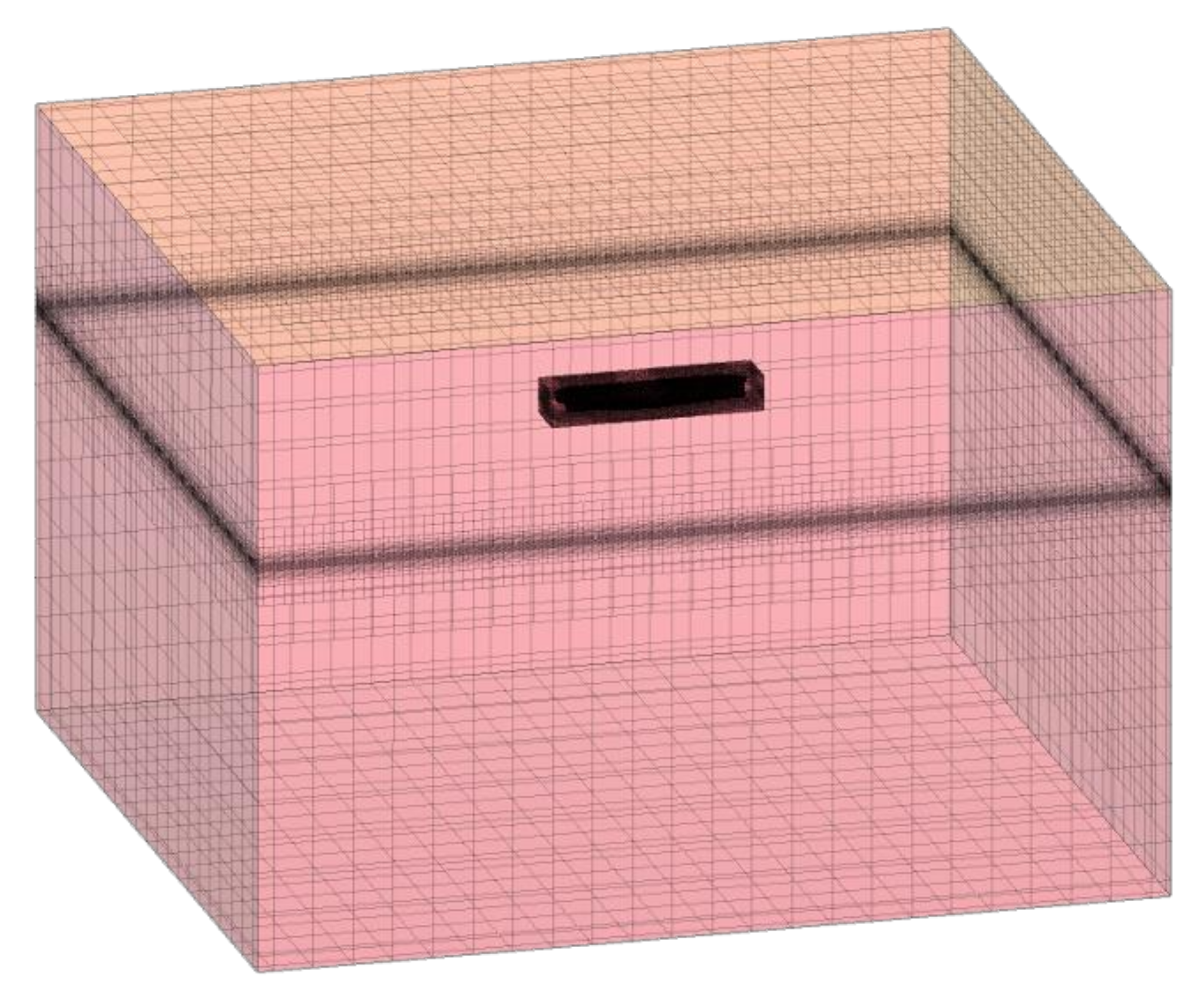
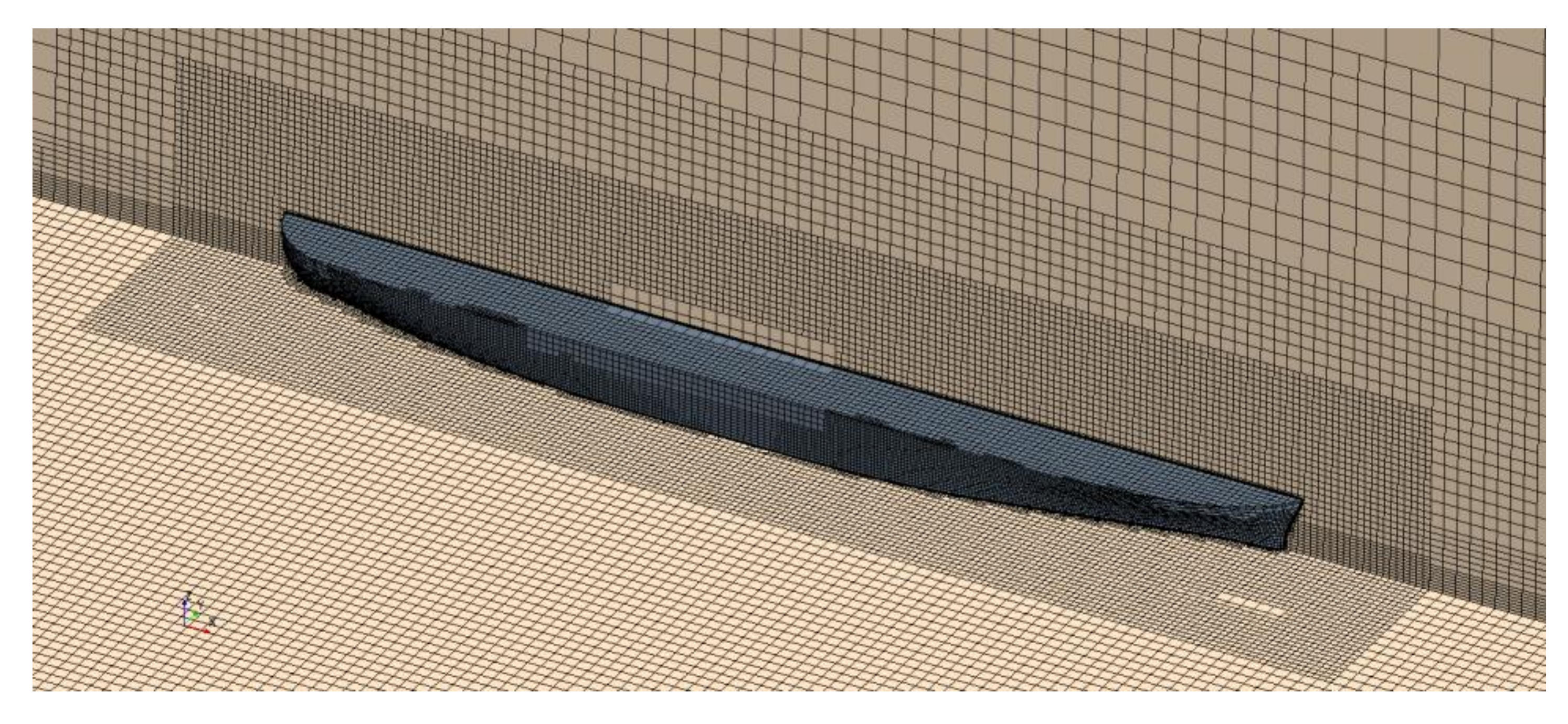
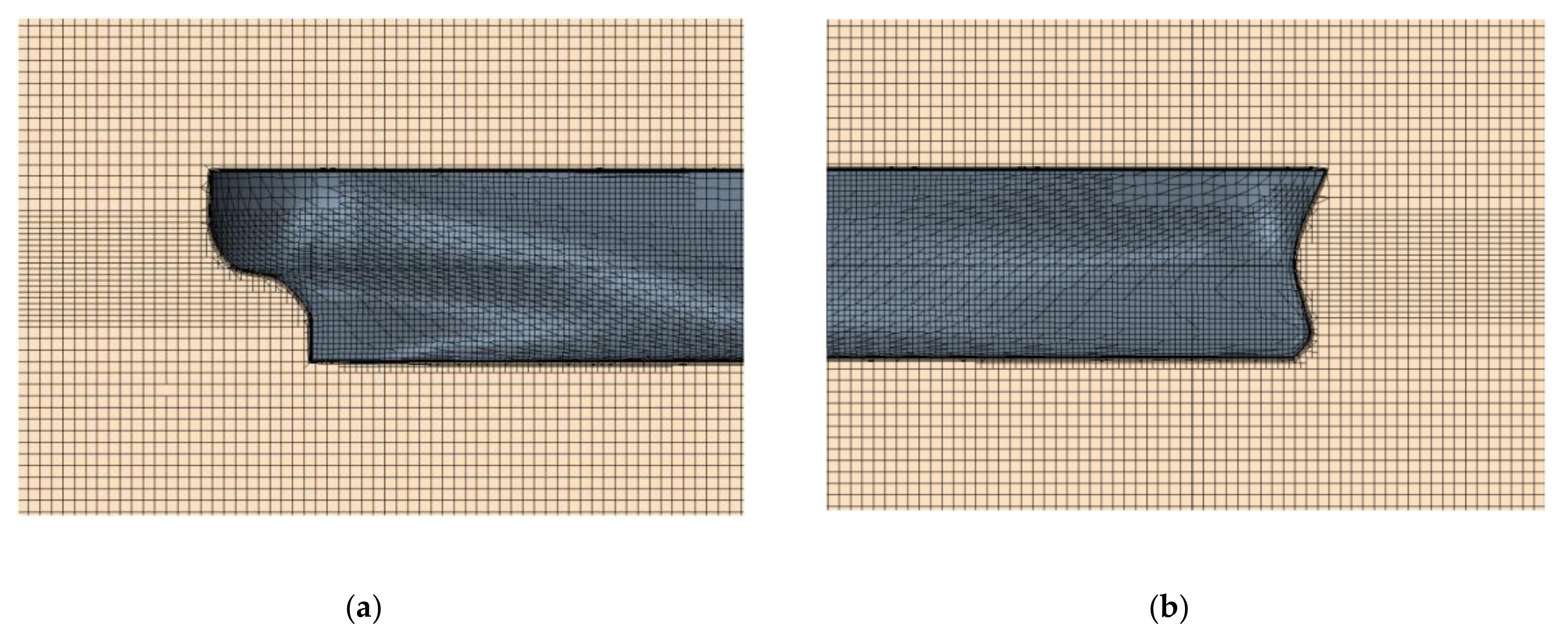
As shown in Figure 6, the fluid domain includes a background region and an overset region. Mesh generation was conducted by the automatic meshing facility in STAR-CCM+. A trimmed cell mesher was employed to produce a high-quality grid for complex mesh-generating problems. The ensuing mesh was formed primarily of unstructured hexahedral cells with trimmed cells adjacent to the surface. The computation mesh has areas of progressively refined mesh size in the area immediately around the hull, as well as the expected free surface, to ensure that the complex flow features were appropriately captured. The refined mesh density in these zones was achieved using volumetric controls applied to these areas. Local mesh was refined around the free surface. At least 16 cell layers are contained within the vertical range of wave height. The horizontal range of per wave length includes 45−150 cell layers for regular waves with wave length ranging from λ/L = 0.6 to 2.0 as a linear ratio scheme. As a result, approximately 4 million cells in total were generated, which turned out to be sufficient for the simulation of the cross wave and ship rigid-body motion responses. Figure 7 shows the refined grid near the free surface and hull body. As shown in Figure 8, the overlapping region consisted of five cell layers of boundary layer mesh near the hull surface (the normalized wall distance y+ value lies in the range of 30−60).
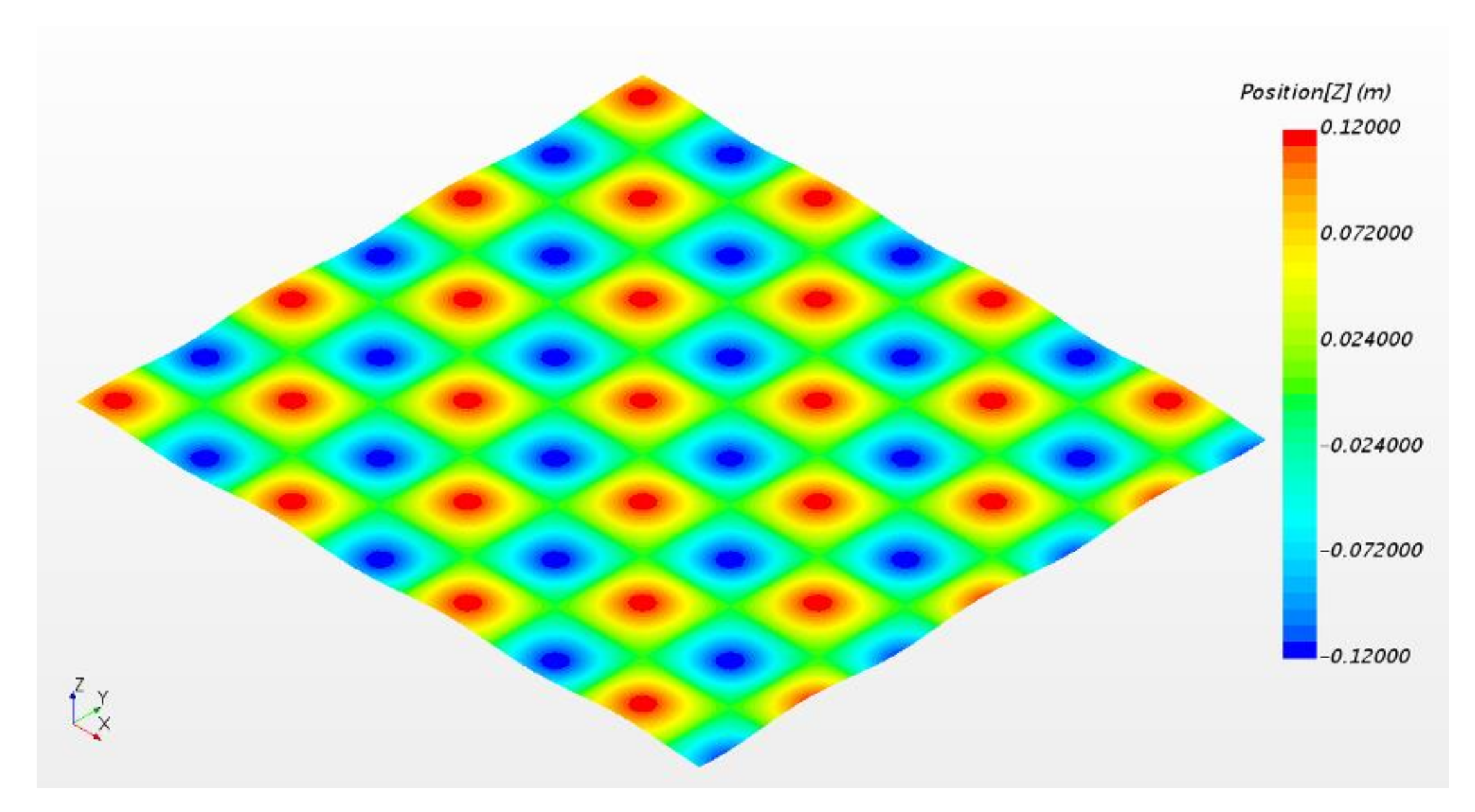
The bi-directional cross wave can be obtained by the superposition of linear regular Airy waves coming from two orthogonal directions. The momentum source-term wave generating method was adopted to formulate the cross wave [20]. This kind of wave generating method can reduce the size of the computational domain and thus reduce the computing effort while not compromising the accuracy and reliability of the solution. Forcing region was applied near the four sidewalls of fluid domain to force the pattern of cross wave [21]. An example of the simulated cross wave field is shown in Figure 9, which shows the wave surface elevation. The figure confirmed that the cross wave simulation was well achieved, and the simulated cross waves are uniformly distributed throughout the tank.
2.3. Simulation Conditions
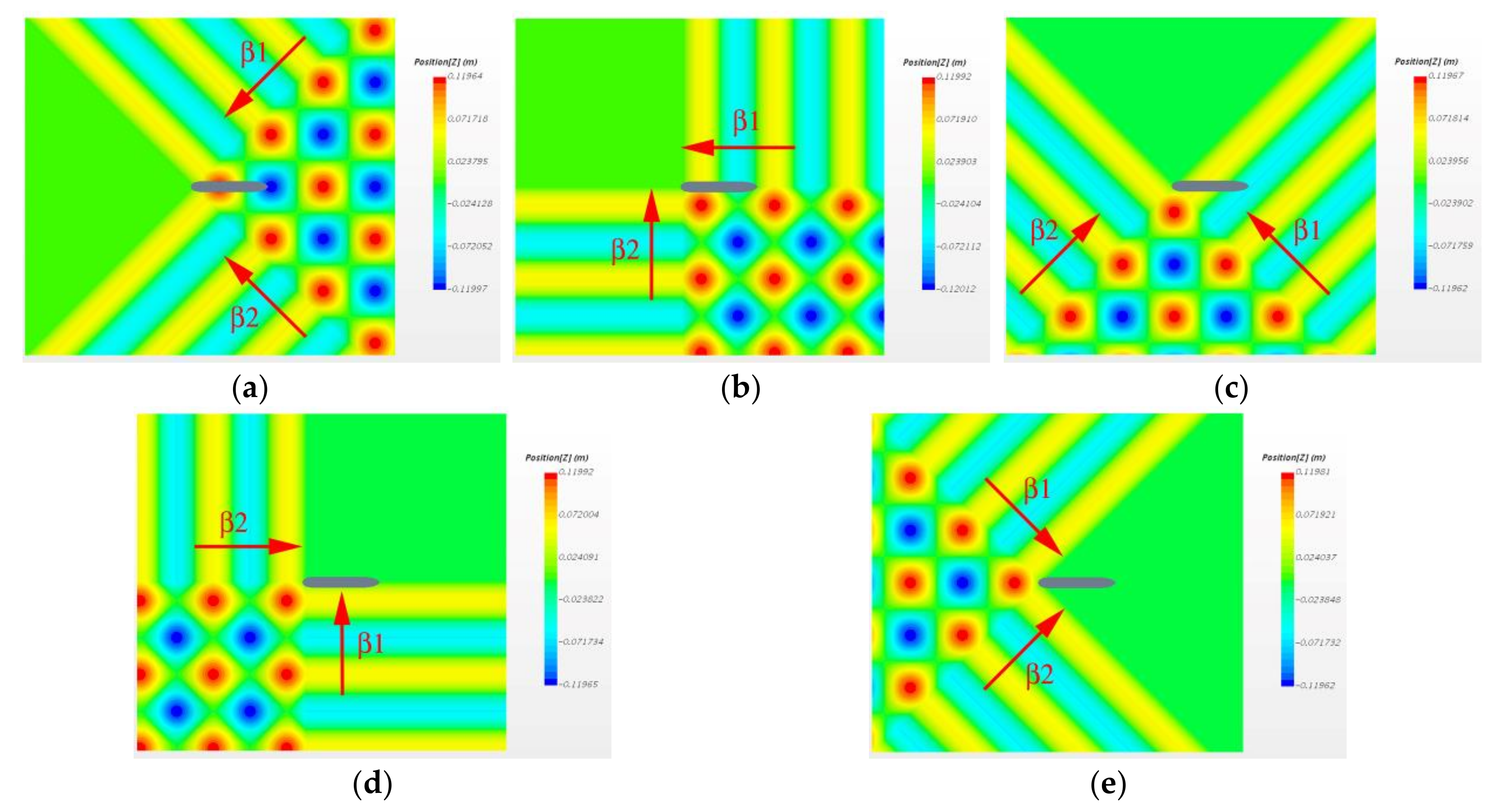
The CFD numerical simulations of ship operating in cross waves have been carried out for different conditions. The involved conditions are summarized in Table 2. For the cross waves involved in this study, the wave lengths (and wave heights) of the two component regular waves are assumed to be identical and they are coming from two directions separated by 90°, i.e., only the monochrome cross wave is involved in this study. Moreover, different wave heading angles with respect to the ship are investigated. The head wave corresponds to 0°, and it increases clockwise, i.e., 90°, 180°, and 270°, corresponding to the starboard beam wave, following wave, and port beam wave, respectively. The ship forward speed is set at Froude’s number of Fn = 0.25 for all cases. In the CFD calculations, for different simulation cases, the ship course angle was unchanged, while different wave heading angle was realized by changing the wave propagation direction of incident waves, which is shown in Figure 10.
The CFD simulations were performed using a computer with Intel Core i-9 CPU, 3.0 GHz, 18 core processors, 64 GB RAM, and 1 TB SSD disk for data writing. The majority of the conditions focus on calculating ship rigid-body motion responses; thus, the time step was set at 0.005 s, which was determined per the Courant number. On average, each of the simulation case took around three days to obtain sufficient time series of ship model’s motions of 16 s. The slamming pressures were involved for calculation only in some typical calculation conditions due to the heavy calculation burden. In these conditions, the time step was set at 0.001 s, which is much smaller than other conditions, in order to capture the impact pressure peak. The mesh was also refined with a total number of over 6 million cells for the slamming involved conditions. Higher mesh resolutions and smaller time step used for slamming pressure study took longer hours. On average, each simulation case took around 30 days for the same simulation period of 16 s.
The iterative convergence of CFD simulation was mainly judged by the residuals and behavior of the simulated signals. In the calculation procedure, the residual decreases gradually and oscillates periodically within a certain range. Moreover, the wave elevation and ship motion signals were also monitored for auxiliary judgment. For example, once the simulation converged, the wave elevation will be consistent with the theoretical value without any signal pollution.
3. Analysis of Cross Waves
The temporal and spatial distributional characteristics of the cross wave are analyzed in this section, which is fundamental for the subsequent ship seakeeping analysis. Due to the orthogonal property of the two component regular waves, the time series of surface elevation of resultant cross wave at any specific point follows a sine function, and it has a same frequency with the component regular wave. The wave amplitude at any specific point within the cross wave field is constant which falls in the closed interval of 0−2A, where A denotes the amplitude of component regular wave. It is noted that in the spatial field of cross wave there are stagnation points where the wave elevation remains zero and time-invariant.
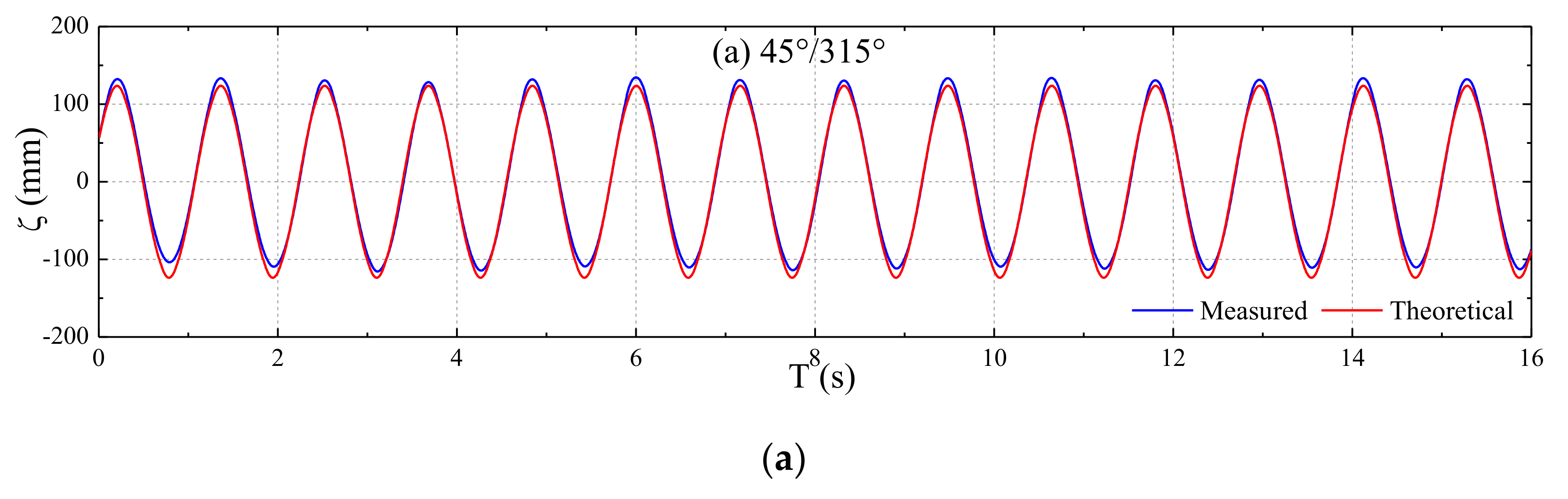
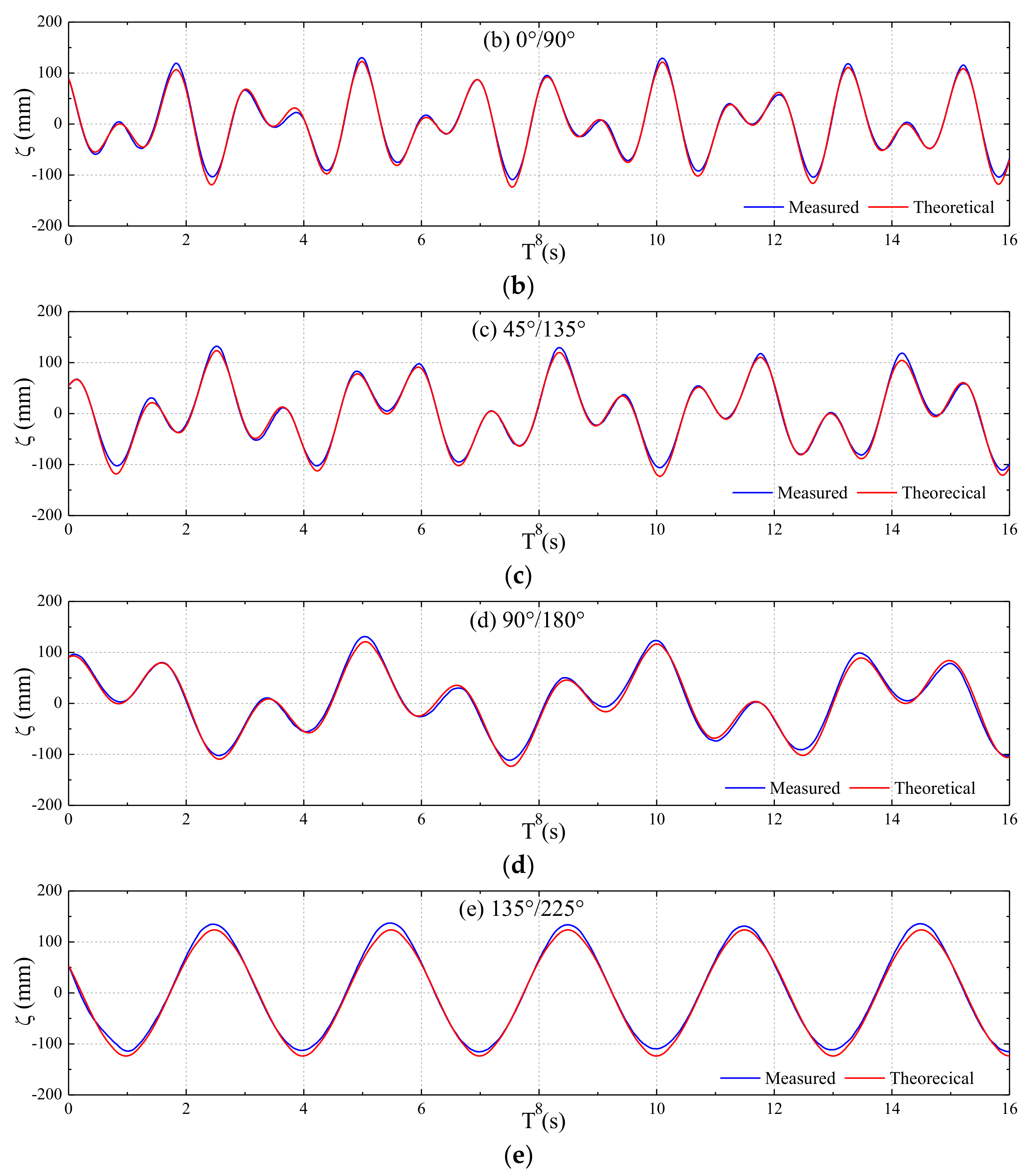
However, the ship encounter wave is quite different from the in situ measurement result, and it depends on ship forward speed, course angle and navigational route. In the numerical wave tank, a wave probe was arranged in front of and with a distance of L/6 away from the ship bow to measure the incoming wave. The measured surface elevation of encounter wave includes the effects of radiation and diffraction due to the present of ship is summarized in Figure 11. This figure includes the cases for ship sailing in different wave headings at constant speed Fn = 0.25 in the same wave field with a wave length of λ/L = 1.0. The theoretical surface elevations of incident wave are also presented in the figures for comparison. As can be seen from the results, the measured data coincide well with the theoretical data of incident wave apart from the surface elevation at crest and trough peaks due to the radiation and diffraction waves in front of the advancing ship. The largest difference between the measured and theoretical value divided by wave amplitude (120 mm) are 16.72%, 13.64%, 14.00%, 10.87%, and 13.87% for the cases of wave heading 45°/315°, 0°/90°, 45°/135°, 90°/180°, and 135°/225°, respectively.
It can be found that the time series of the encounter wave for ship advancing with wave heading 45°/315° or 135°/225° are monochromatic and sinusoidal, while the time series for the remaining three wave heading cases (0°/90°, 45°/135°, 90°/180°) are bichromatic and irregular. This can be explained by the fact that the ship encounter wave can be regarded as the superposition of two encounter component waves. For the cases of wave heading 45°/315° or 135°/225°, the encounter frequencies of the two component waves are identical; for the remaining three cases, the encounter frequencies of the two component waves are not identical. The encounter frequency of component wave can be obtained by
where ω denotes wave frequency, ωe denotes wave encounter frequency, U denotes ship speed, β denotes wave heading angle, and g denotes acceleration of gravity.
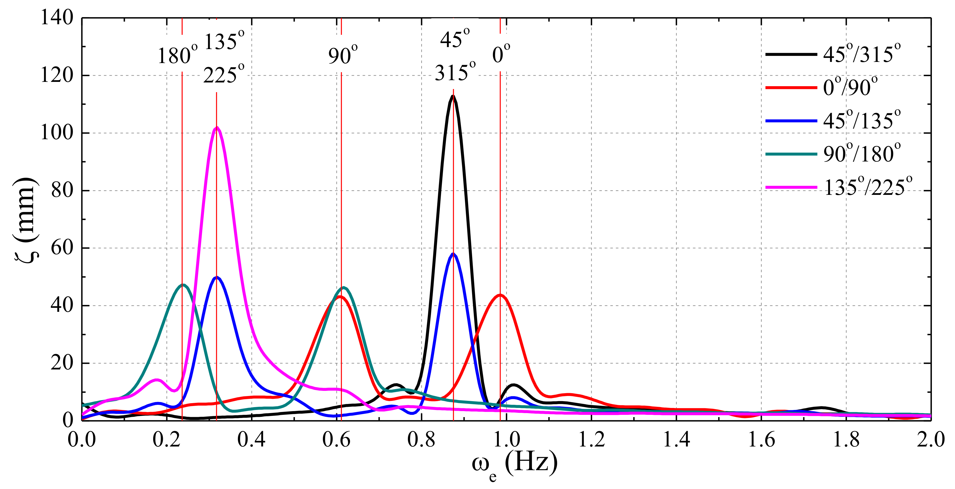
The frequency domain results of the ship encounter wave obtained by applying fast Fourier Transformation (FFT) of the time series data for different wave heading cases are summarized in Figure 12. The peak frequency can be identified from the vertical auxiliary red lines. As is seen from the curves, the peak frequency of encounter wave coincides well between the curves for different wave headings. The peak value of the curve for 45°/315° or 135°/225° that induced by two symmetric component waves is approximately double of the response peak value induced by asymmetric component wave due to the linear superposition effect of component waves. Moreover, a comparison of the peak frequency in Figure 12 against the encounter frequency obtained by Equation (1) is summarized in Table 3. The results indicate that the difference increases from 1.44% to 5.83% with the decrease of encounter frequency. The reason is that, in the case of head wave 180°, the ship speed is consistent with the wave propagation direction. Thus, the incident waves get superposed with the more diffraction wave, radiation wave, and ship steady wave, which affects the peak frequency of the incoming wave.
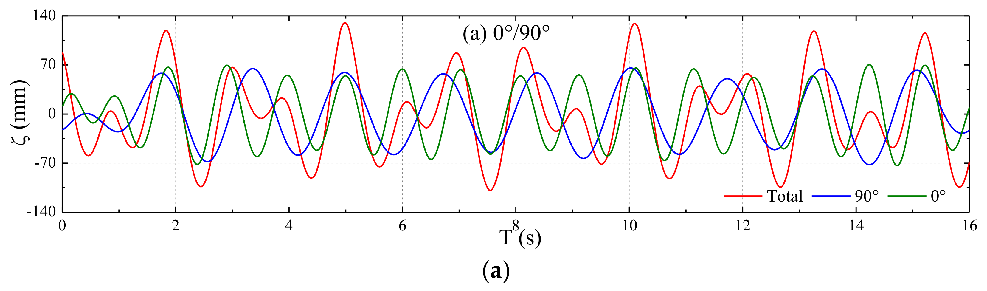
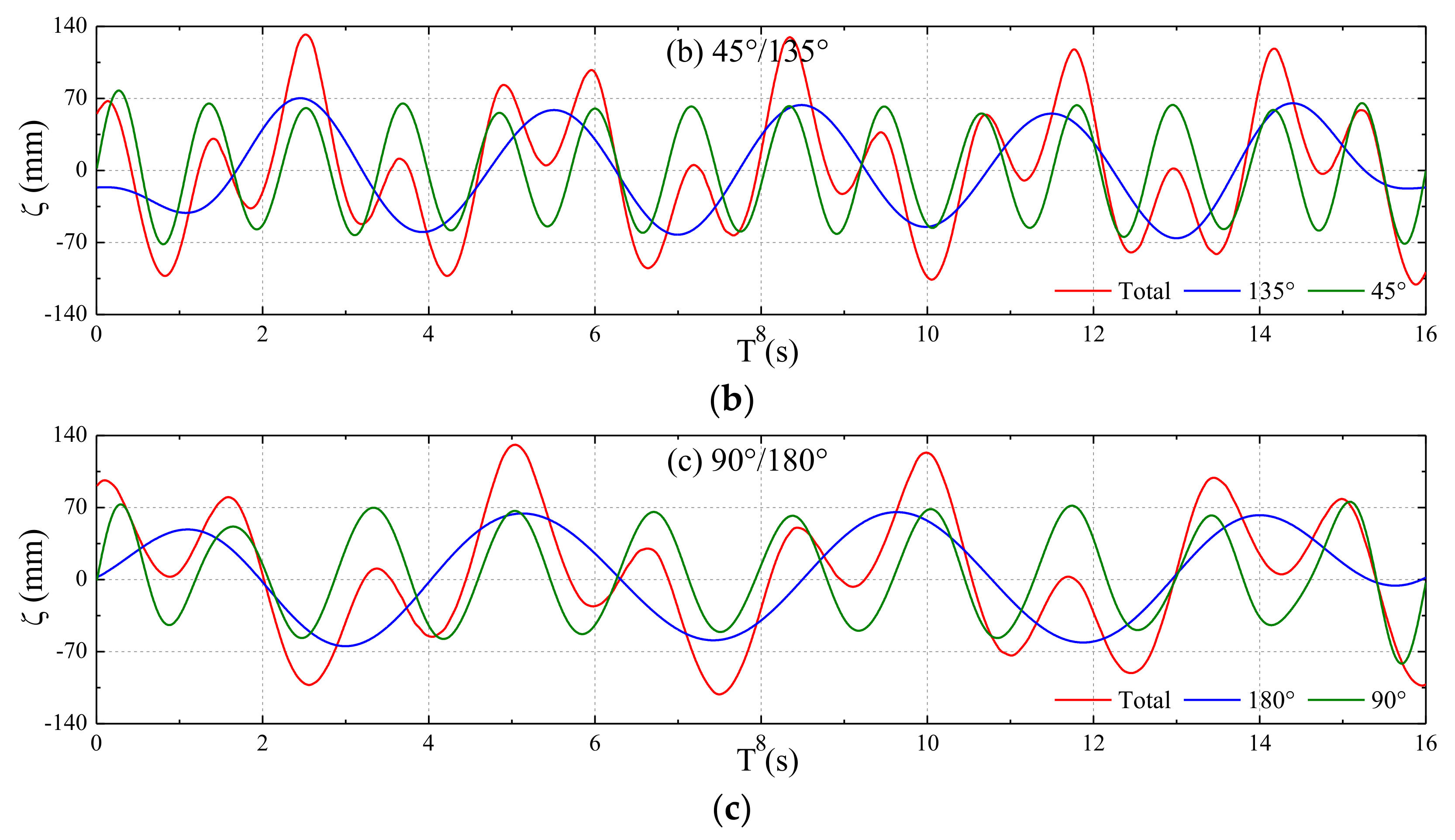
A band-pass filter was used to separate the component waves from the measured total cross wave for the three asymmetric wave heading cases. The cut-off frequency was set at 0.8 Hz, 0.6 Hz, and 0.4 Hz to divide the low- and high-frequency component wave for the cases of wave heading 0°/90°, 45°/125° and 90°/180°, respectively. As shown from the results in Figure 13, all the component waves show regular behavior with nearly the same amplitude of 60 mm. The results confirm that the cross wave can be regarded as the linear superposition of two component regular waves.
4. Analysis of Ship Seakeeping Behavior
Ship seakeeping behavior in the cross wave is systemically analyzed in this section. The CFD algorithm is preliminarily validated by comparing with experimental data of ship vertical motions in head regular waves. Then, ship motion responses and green water on deck in different cross wave fields are systemically analyzed. The impact pressure on the bow area induced by cross waves in typical conditions is also analyzed by the calculation results of the refined grid scheme. The results also indicate that ship motion response in a cross wave can be quite large, which is different from that induced by a uni-directional regular wave. It is worth mentioning that a comparative study on the ship’s motion behavior in uni- and bi-directional waves has been conducted and reported in the authors’ recently published paper [22].
4.1. Validation of the CFD Numerical Model
Some worldwide state-of-the-art wave basins are equipped with a two-side wave maker, which can be used for the generation of a cross wave. However, until now, ship seakeeping test in a cross wave has not been conducted or reported. Therefore, in this section, the developed CFD algorithm for ship seakeeping prediction is validated by comparison with some existing experimental data of ship motions in head regular waves presented by Fonseca and Guedes Soares [23].
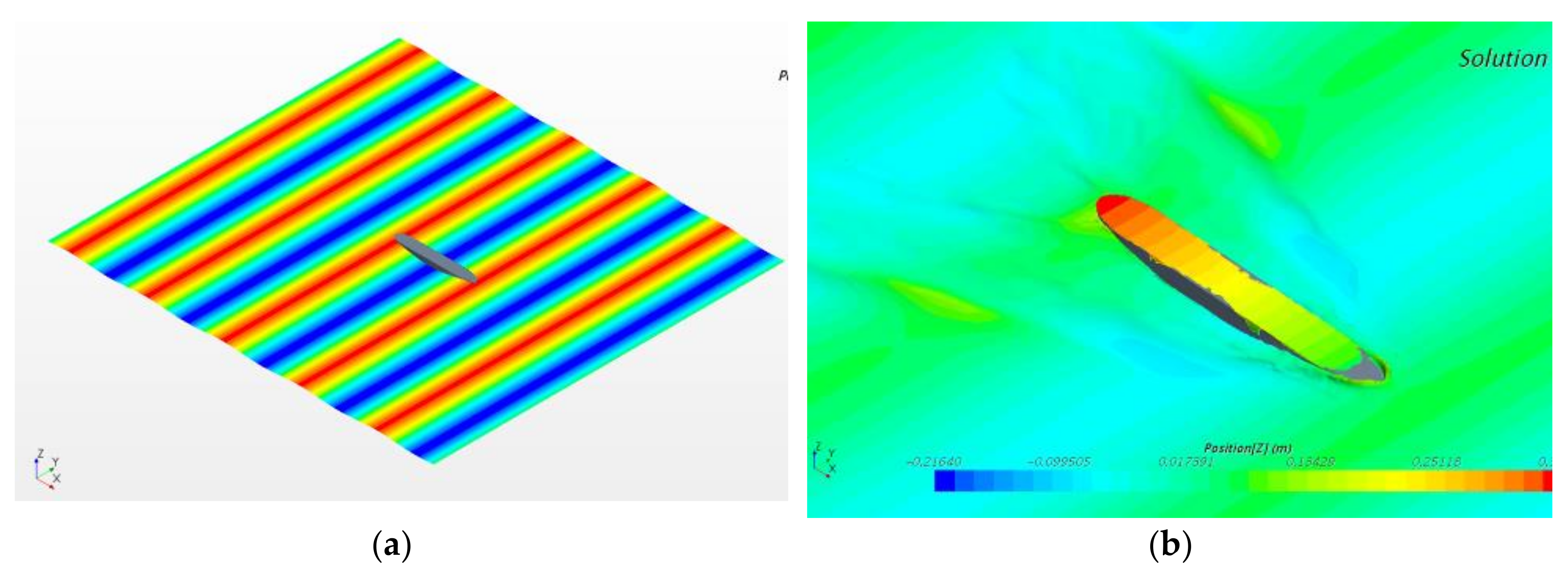
The tests were conducted at the Laboratory of Ship Dynamics of the El Pardo Model Basin in Madrid, Spain, which is 150 m long by 30 m wide by 5 m deep. The experimental S175 ship model has the same dimensions as the numerical model used in this study. The ship speed Fn = 0.25 and wave amplitude 60 mm are selected in both the experiment and numerical simulation for the sake of consistence. The ship heave and pitch motions in regular waves at different wave length range conditions are compared. It is worth mentioning that the numerical details including the mesh generation, wave making, and ship motion simulation methods in the regular wave cases are consistent with those in the cross wave cases. An example of the CFD simulated regular wave interaction with ship in a head wave case is shown in Figure 14.
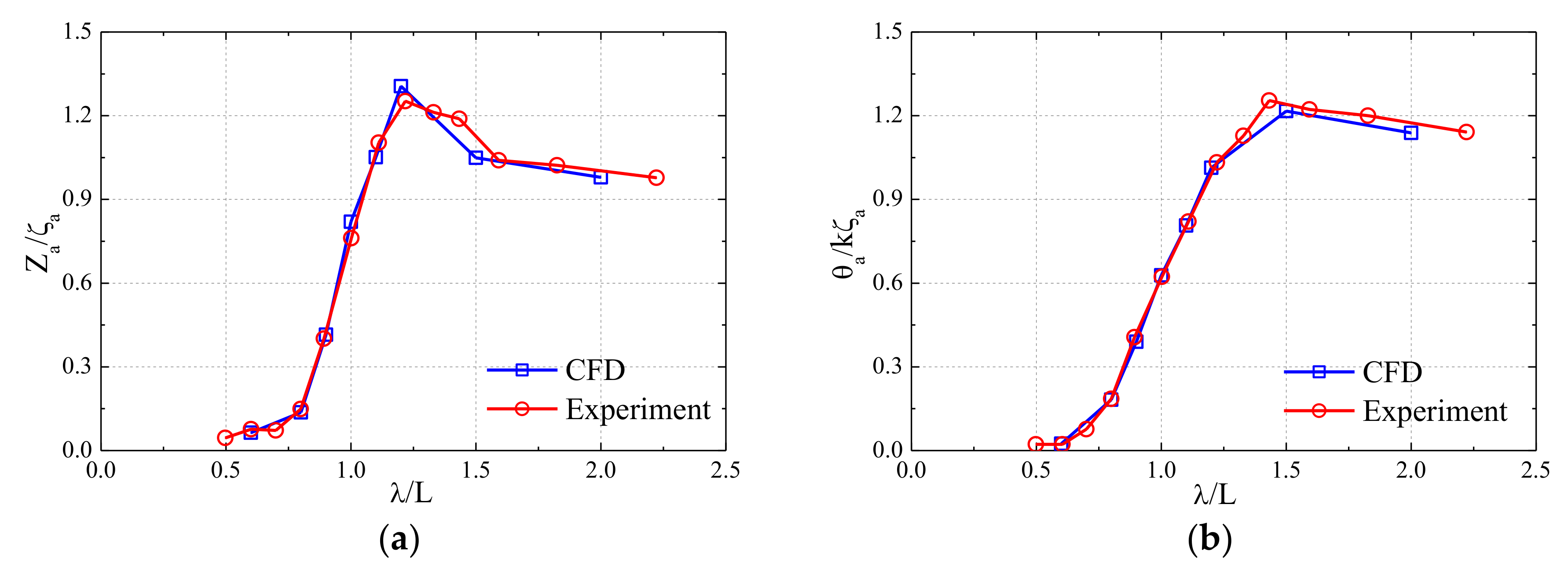
The comparative response amplitude operators (RAOs) of heave and pitch for the ship sailing in the head regular wave by experiment and numerical simulation are shown in Figure 15. As seen from the curves, the results confirmed that the ship motion responses predicted by the CFD solver coincide well with the experimental data even though there exist small difference near the peaks of the curve. The CFD numerical result overestimates the heave value by 4.25% at the peak of curve (at λ/L = 1.2). The experimental pitch value is slightly greater than the numerical data for the cases of λ/L > 1.2 and the largest difference 6.39% occurred at the peak of curve (around λ/L = 1.4).
4.2. Influence of Wave Heading on Ship Motions
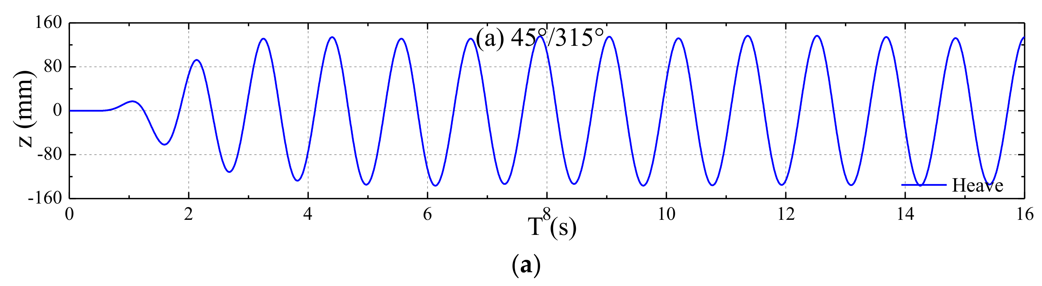
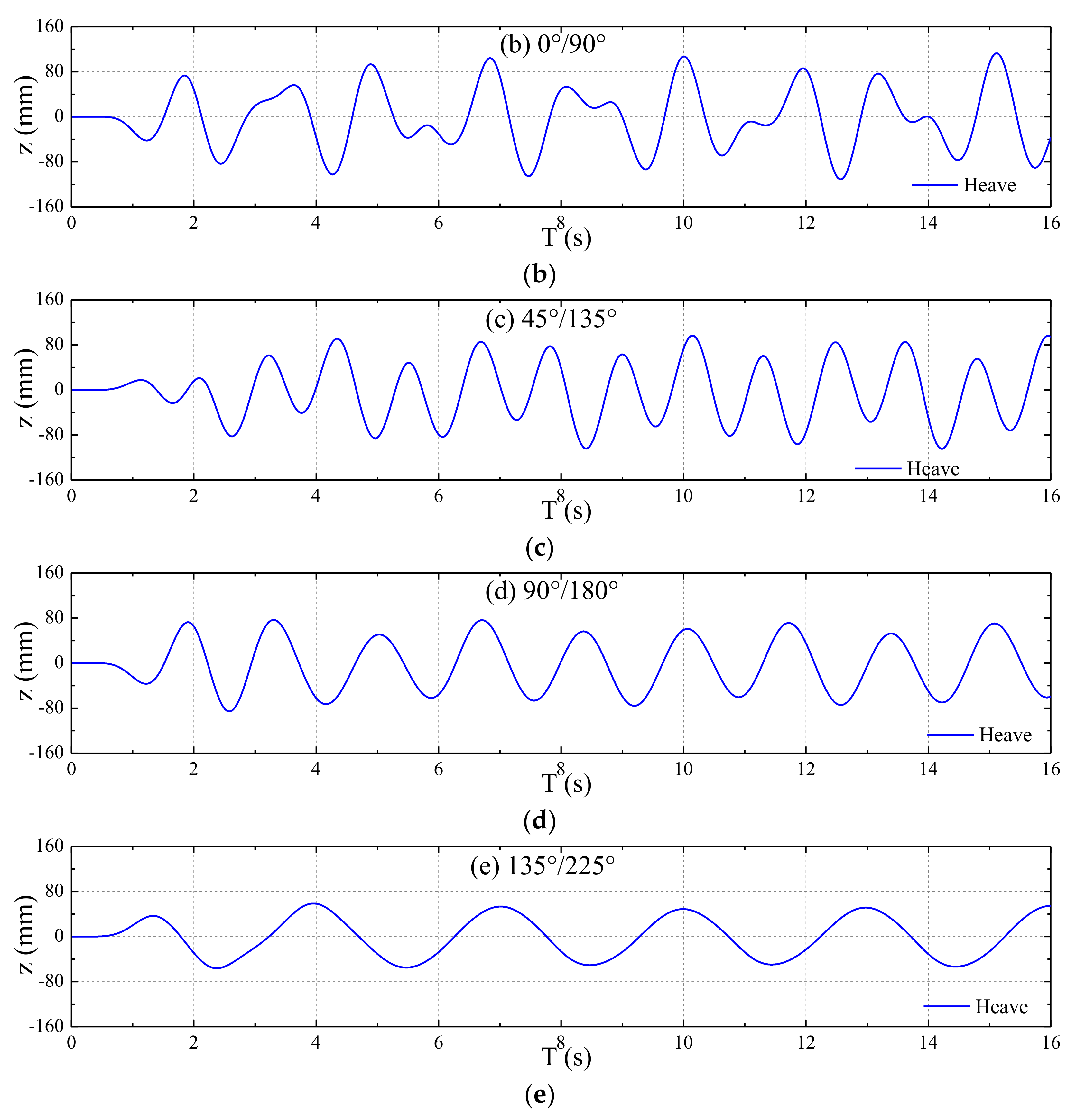
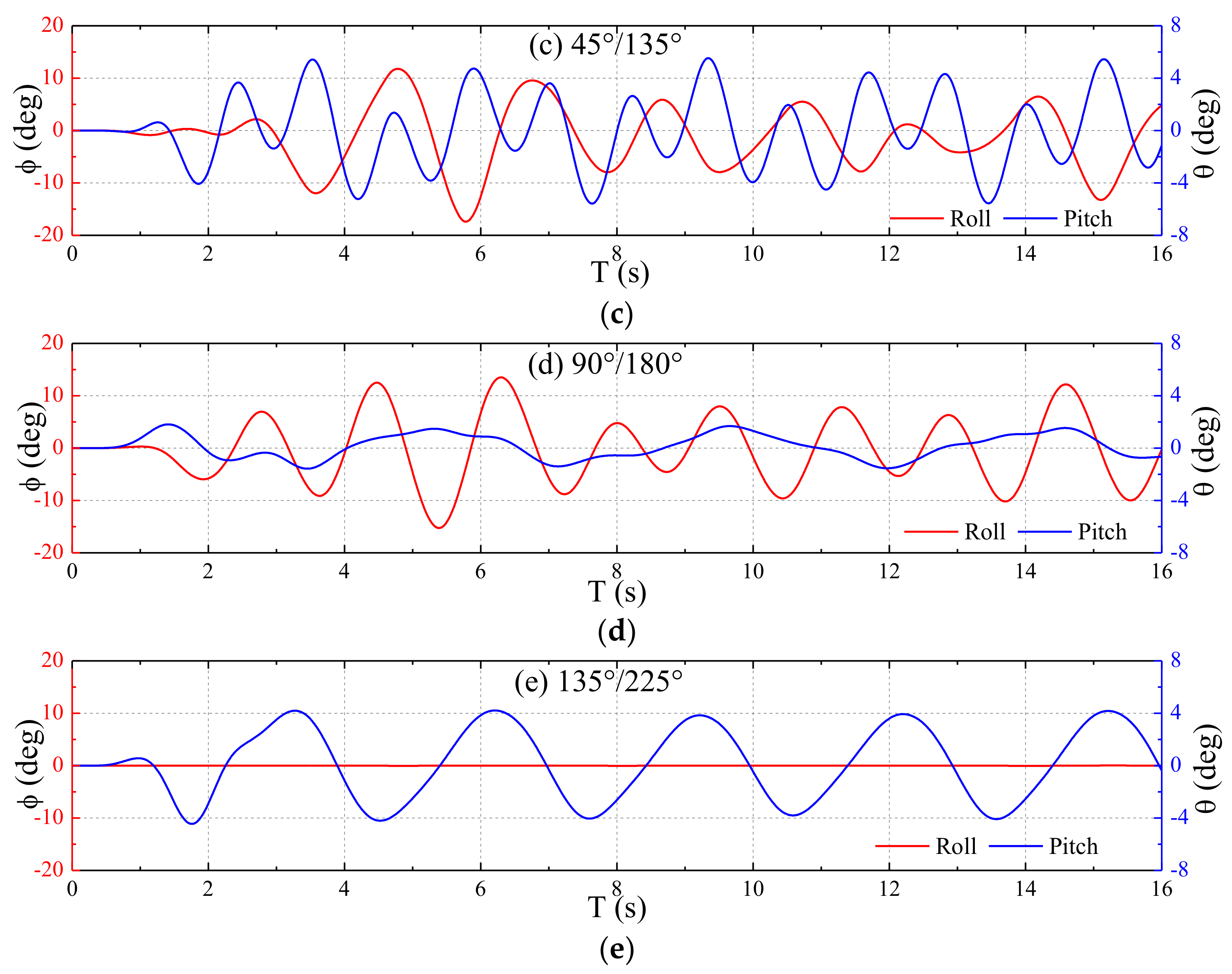
The simulated time series of heave, pitch, and roll motions for the ship sailing in the cross wave field (λ/L = 1.0) at speed Fn = 0.25 at different wave headings (45°/315°, 0°/90°, 45°/135°, 90°/180°, and 135°/225°) are shown in Figure 16 and Figure 17.
As can be seen from the results, the heave motion signal for ship sailing at wave headings 0° (45°/315°) and 180° (135°/225°) is regular or sinusoidal. Both the amplitude and frequency of the heave signal at wave heading angle 0° (45°/315°) is much greater than that of 180° (135°/225°). On the other hand, the heave signal of the ship sailing at wave headings 45° (0°/90°), 90° (45°/135°), and 135° (90°/180°) is irregular and bichromatic. However, the bichromatic behavior of the ship sailing at wave heading 135° (90°/180°) is weak since the following component wave of 180° contributes less to the total heave response and the heave is mainly induced by the beam component wave of 90°.
Moreover, due to the symmetry of the incident wave, the roll motion is zero when the ship is sailing at wave heading 0° (45°/315°) or 180° (135°/225°), while the corresponding heave and pitch motion are regular. However, the roll and pitch motions for ship sailing at wave headings 45° (0°/90°), 90° (45°/135°), and 135° (90°/180°) are irregular or bichromatic, and the peak value of the roll is generally much larger than the pitch value for each case. The pitch response is small, with the largest value of 1.81° in the case of wave heading 135° (90°/180°) since the encounter frequency is far from its natural frequency. It is noted that the roll motion does not show steady behavior within the 16 s period. This is because the natural period of roll motion is relatively large, but the cycle period of roll encountered by the ship within 16 s is limited. Since the CFD simulation time is not long enough due to computational cost limitation in this study, a longer simulation will be performed in future work to obtain more insightful conclusions.
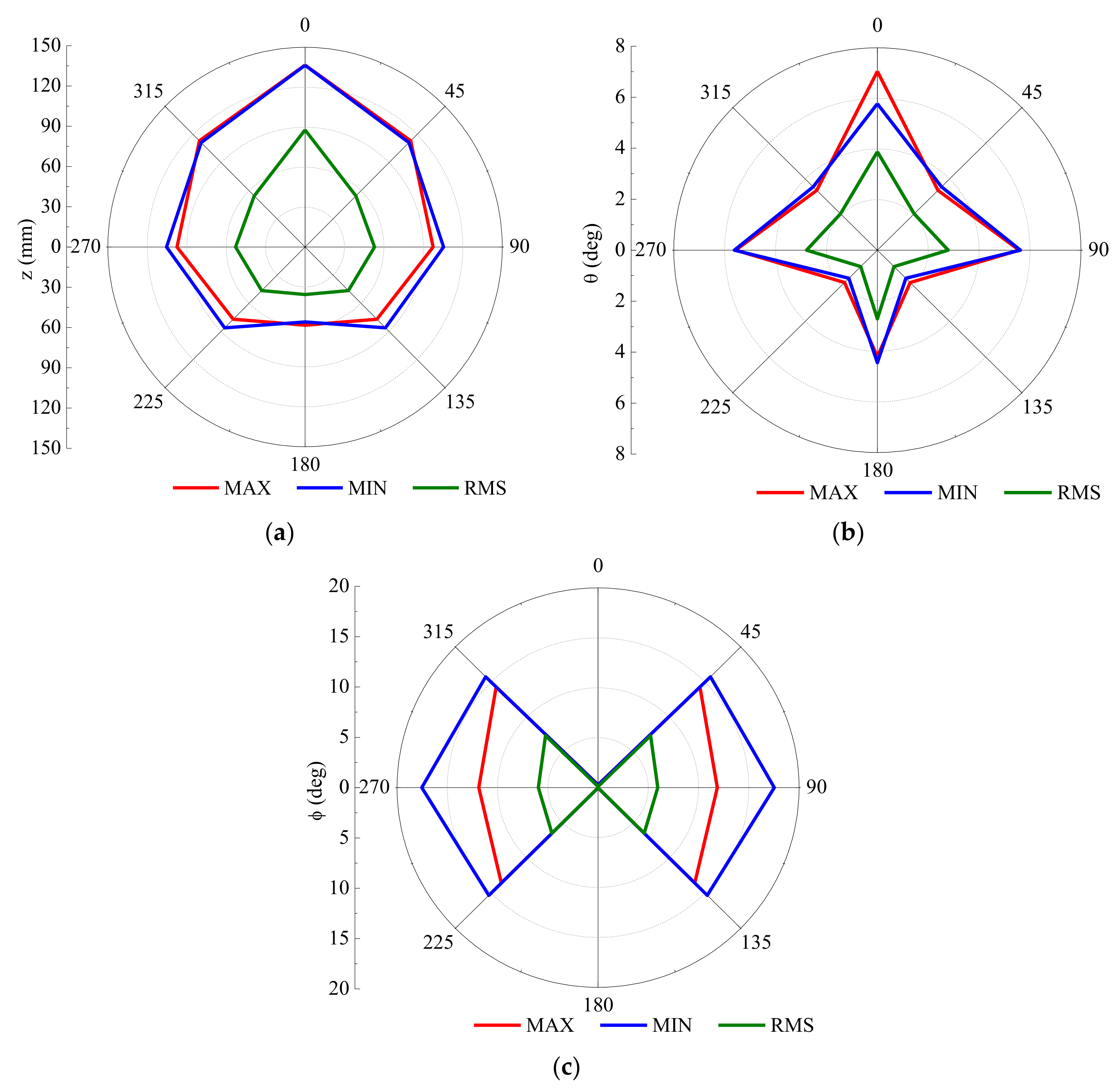
The largest crest and trough peak values and the root mean square (RMS) of time series of ship motions within the 16 s varying with different resultant wave headings are summarized in Figure 18. Note that the polar angle in the polar coordinate denotes resultant wave heading of two component waves. As seen from the results, the largest heave and pitch response occur at resultant wave heading 0° (45°/315°). The second largest response values for heave and pitch occur at resultant wave heading 45° (0°/90°) and 90° (45°/135°), respectively. The lowest heave and pitch responses occur at resultant wave heading 180° (135°/225°) and 135° (90°/180°), respectively. The roll response value remains zero for the symmetrical wave heading case of resultant wave heading 0° (45°/315°) and 180° (135°/225°). The roll motion time series is not as steady as the pitch motion signal. The difference among the roll response statistical values in the three cases of resultant wave heading 45° (0°/90°), 90° (45°/135°), and 135° (90°/180°) is relatively small, and the largest peak (MAX) value lies in the narrow range of 15.25°−17.39°.
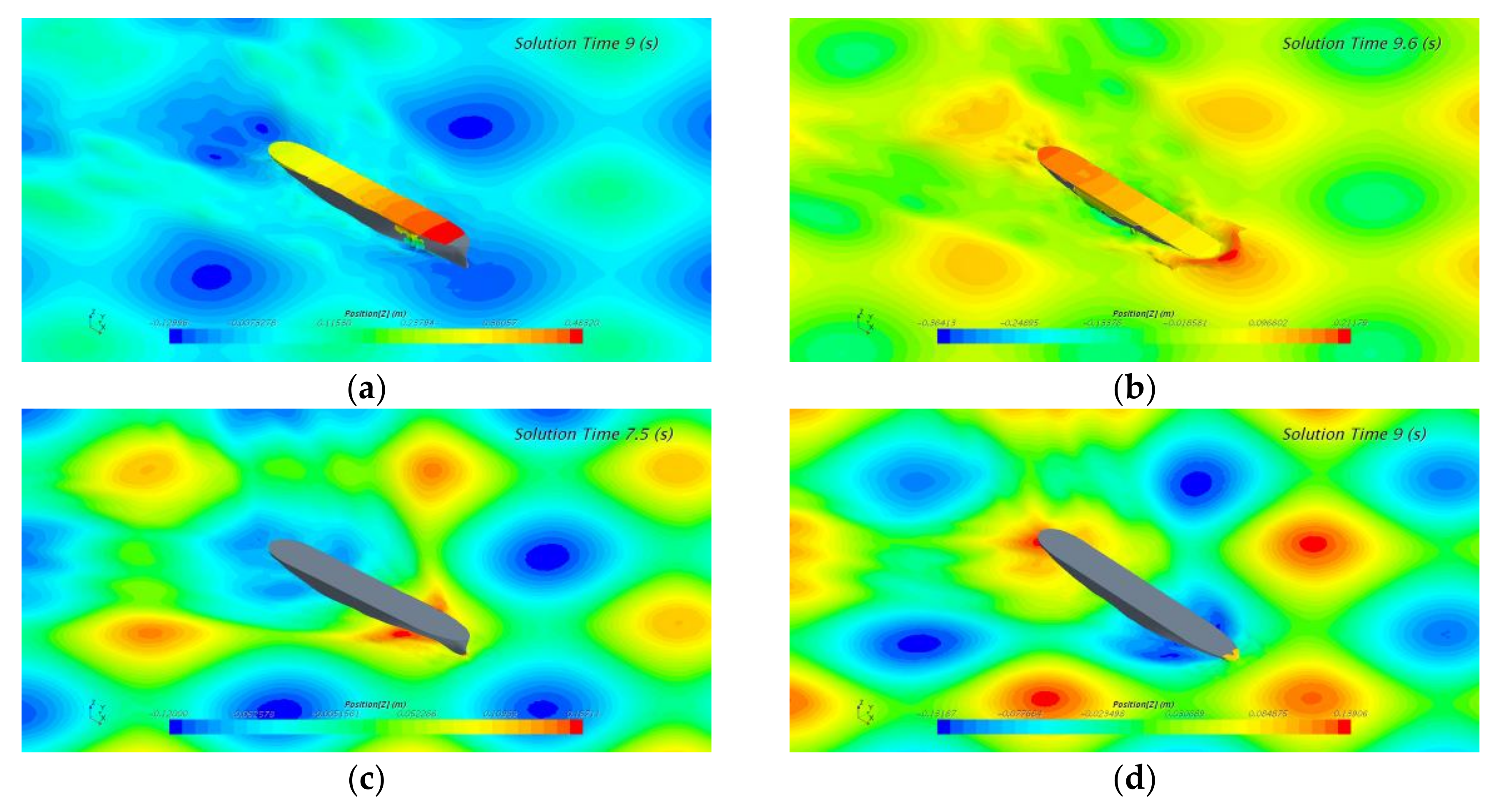
The severest vertical motion of the ship occurs in the resultant head wave condition 0° (45°/315°). The RMS value of heave and pitch for a ship sailing at the wave heading 0° (45°/315°) is, respectively, about three and two times as large as the value for the wave heading 180° (135°/225°). For a better understanding of the ship wave interaction problem, a comparison of the large amplitude longitudinal motion and green water on deck for a ship in the two symmetric wave conditions is shown in Figure 19. The figure includes two phases of ship motion state, which are bow up and bow down motions. As can be seen from the figures, severe green water on deck occurred when the ship was sailing in the wave heading 0° (45°/315°), and the water even overtopped and scoured the whole deck from bow to stern. However, due to the relatively small pitch and heave motion, only slight green water occurred when the ship was in a bow down motion phase at the wave heading 180° (135°/225°).
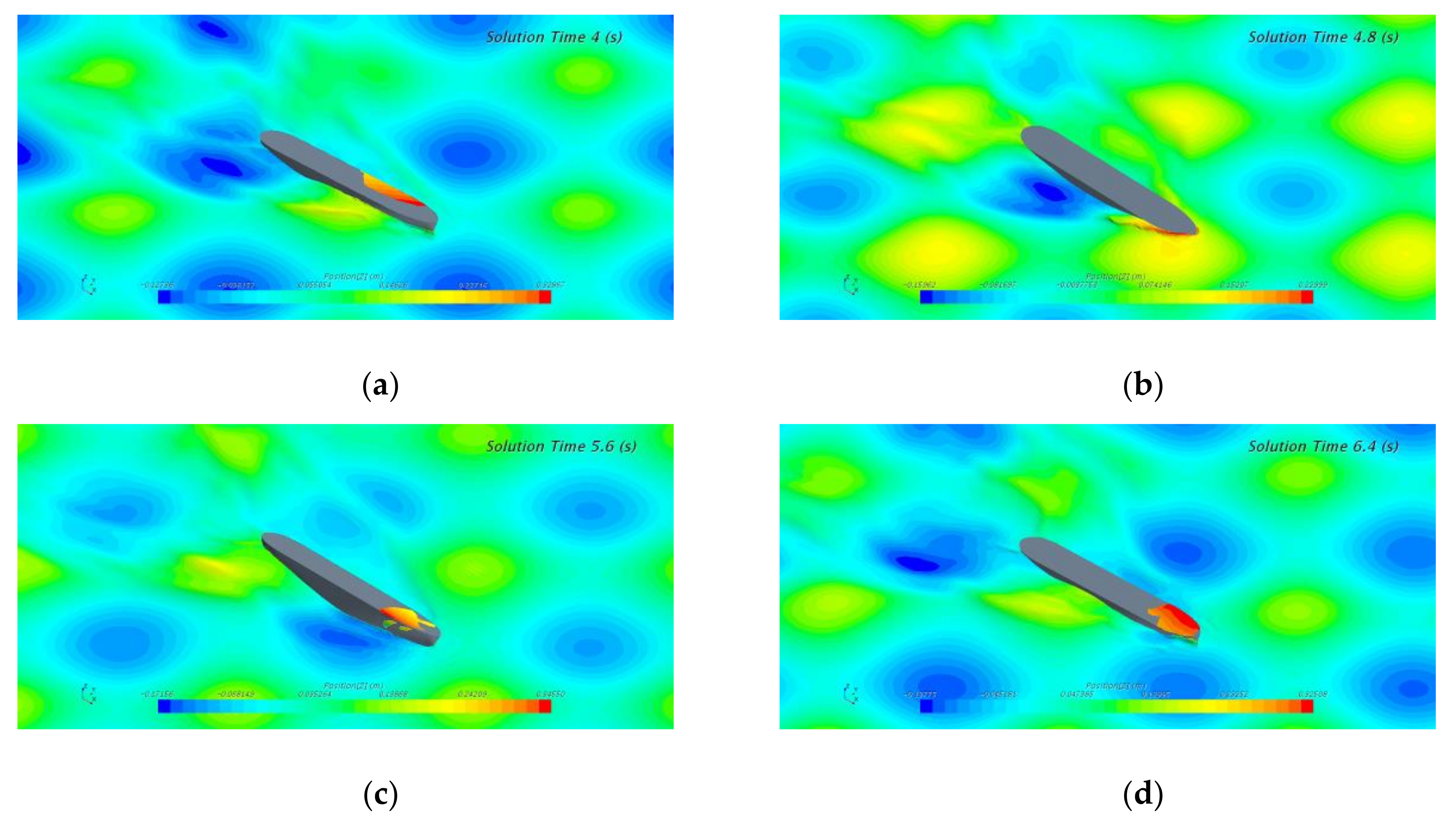
To be different from the large amplitude vertical motion of ship in the symmetrical waves, significant roll motion would occur for a ship sailing in the asymmetrical waves. The large amplitude roll motion procedure of a ship sailing in the wave heading 90° (45°/135°) is depicted in Figure 20. It can be observed that the water scoured onto the deck from the port side and ran out from the starboard side due to the coupled effect of pitch and roll motions. The green water for a ship in the wave heading 90° (45°/135°) is not as severe as that in the head wave condition 0° (45°/315°), and the reason is twofold: first, the vertical acceleration on deck is lower for ship in the wave heading 90° (45°/135°); second, the roll period is much larger than pitch period even though the roll amplitude is relatively large. Thus, the large roll will not result in so violent a flow on deck as that of the pitch motion.
4.3. Influence of Wave Length on Ship Motions
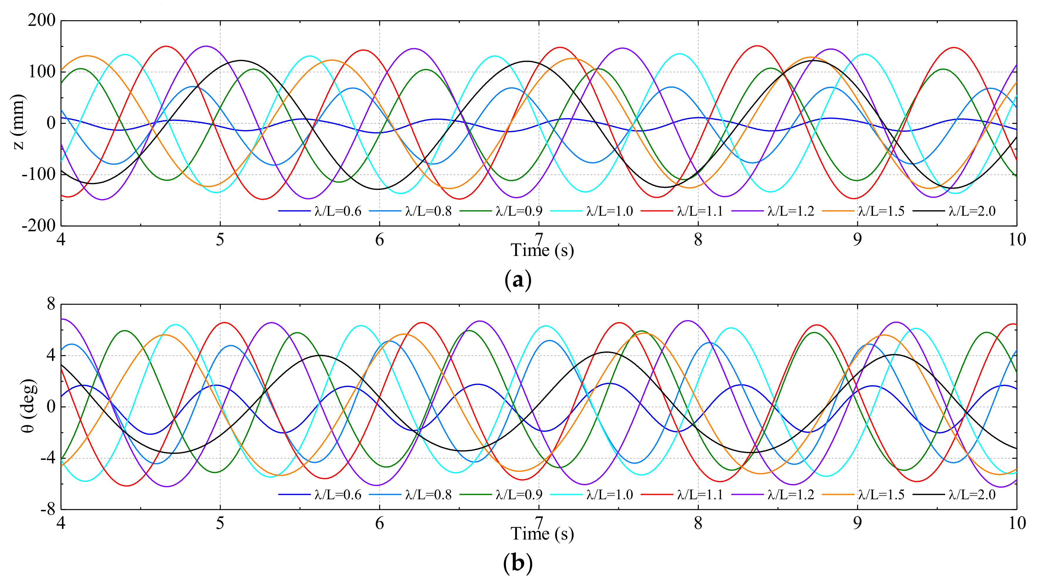
As concluded from the above analysis, the severest heave and pitch motions generally occur when ship sailing at the wave heading 45°/315°. The time series of ship heave and pitch motions at different wave lengths λ/L = 0.6−2.0 for wave heading 45°/315° and ship speed Fn = 0.25 are summarized in Figure 21. As it is seen from the time series, the vertical motion signals are generally regular and sinusoidal, with different amplitudes and different encounter frequencies.
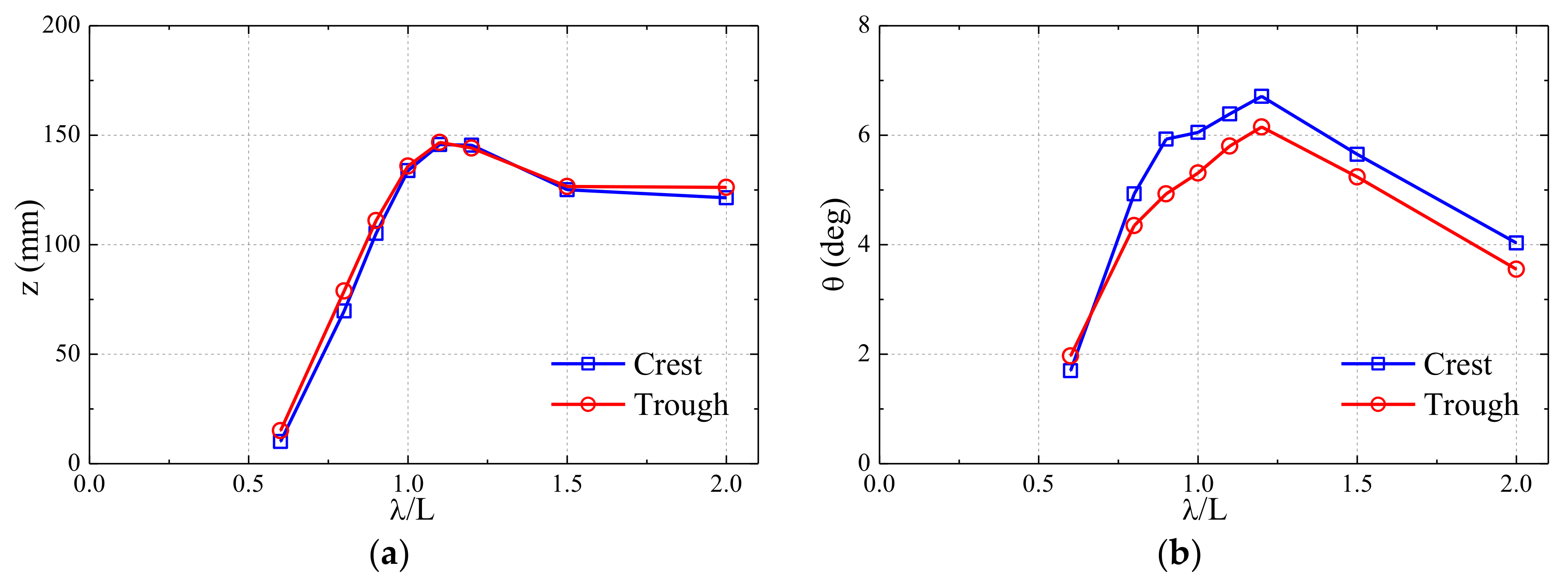
The amplitude of ship vertical motions in different wave lengths λ/L = 0.6−2.0 at the wave heading 45°/315° is summarized in Figure 22. The results indicate that the heave increases from λ/L = 0.4 to 1.0 almost linearly, and the largest heave amplitude of 146.7 mm appears at λ/L = 1.1. The heave amplitude trends steadily with a same value of the wave amplitude 120 mm when λ/L is greater than 1.5. The largest pitch amplitude 6.71° occurs at λ/L = 1.2 and decreases rapidly with the increasing λ/L. To summarize, the largest vertical motion response occurs when the encounter frequency is at or near the natural frequency of ship. The forward speed also contributes to the vertical motion especially for the cases around the peak.
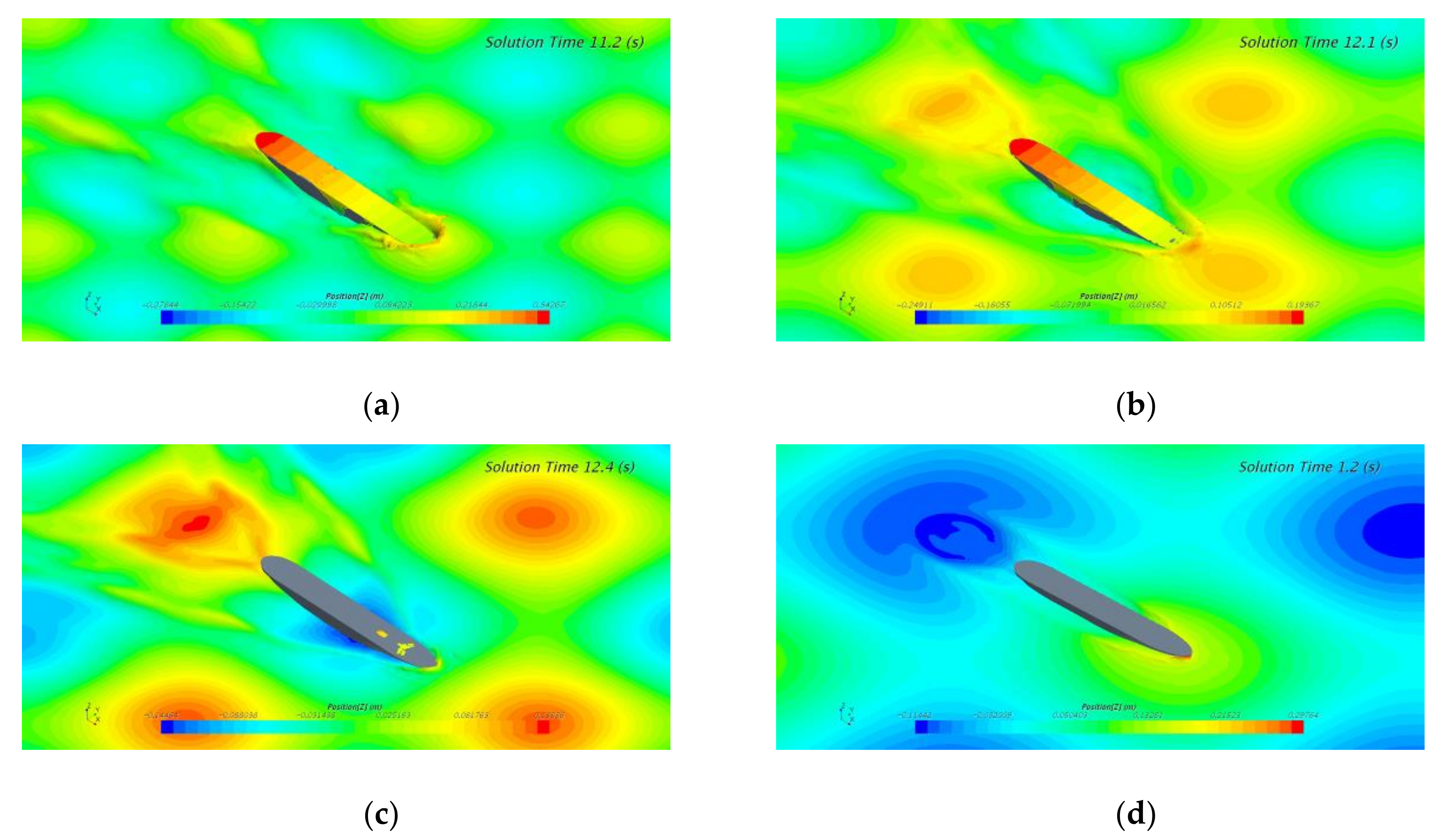
The green water on deck phenomenon for ship sailing in the wave heading 45°/315° at four typical wave lengths of λ/L = 0.8, 1.2, 1.5, and 2.0 is compared in Figure 23. The figures reveal that the severest green water occurred in the case of λ/L = 1.2. This can be explained by the fact that a severe slamming event and green water on deck occurred when the encounter frequency is at or near the ship motion’s resonant frequency. The green water on deck in the cases of λ/L = 0.8 and 1.2 is quite harsh. The heave and pitch motion response in the range of λ/L = 0.8–1.2 are also relatively high (see Figure 22), which results in the severe slamming and green water on deck. Only slight deck wetness occurred in the case of λ/L = 1.5, and no green water occurred in the case of λ/L = 2.0.
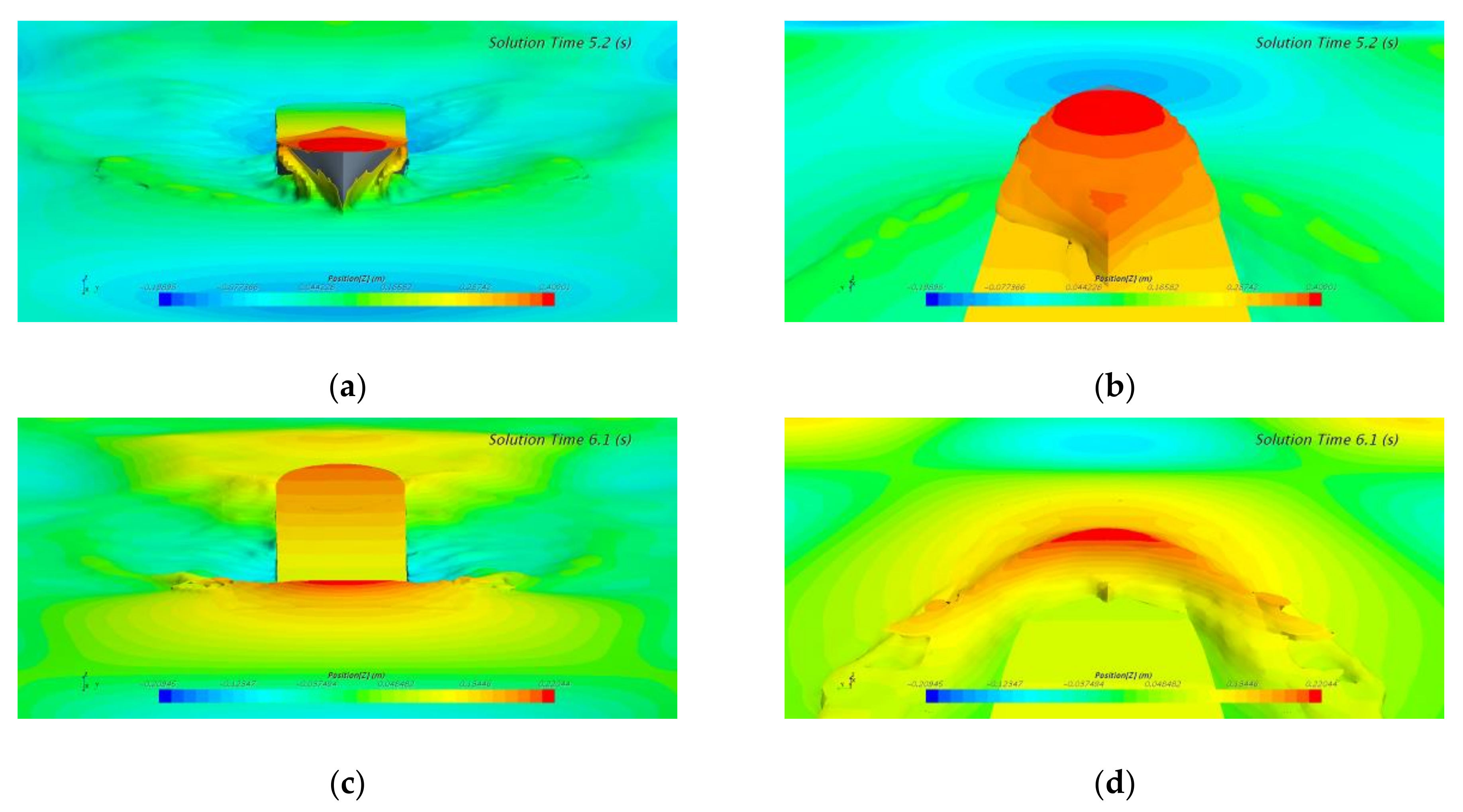
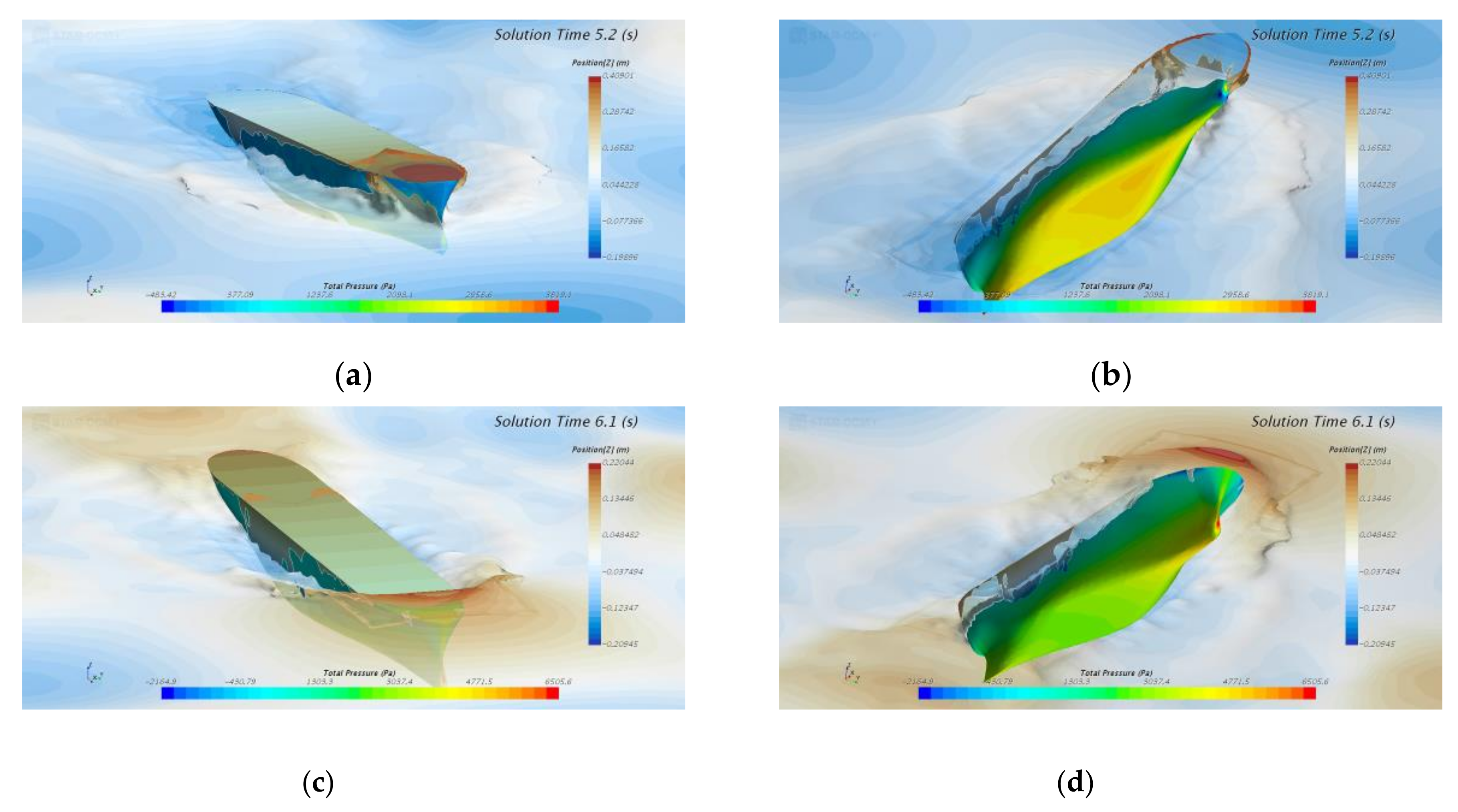
In addition, a view of ship slamming and green water procedure within one encounter period for ship sailing in the wave condition of λ/L = 1.2 is shown in Figure 24 and Figure 25. The figures reveal that the water overtopped and scoured the whole deck from bow to stern. These figures also clearly reveal that the breaking waves and the splashing water have been successfully captured by the CFD simulation.
5. Slamming Pressure on Ship Bow Area
The distribution of wave impact pressure on the bow area for the ship sailing in a cross wave is investigated in this section. Two typical conditions including the ship sailing in both symmetric and asymmetric cross wave fields are selected for investigation.
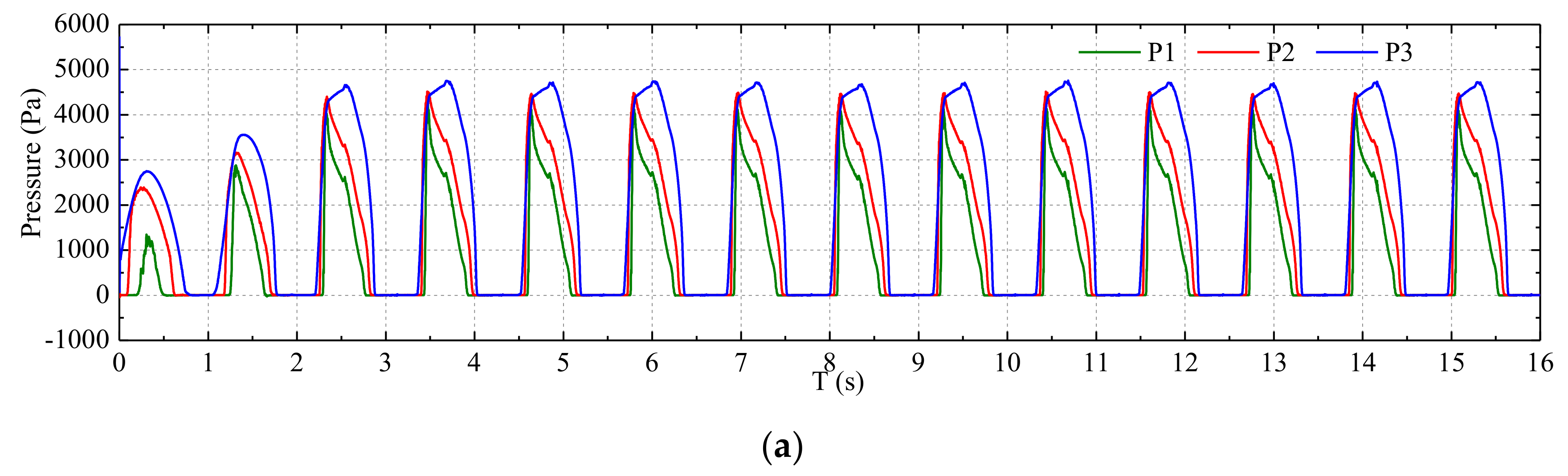
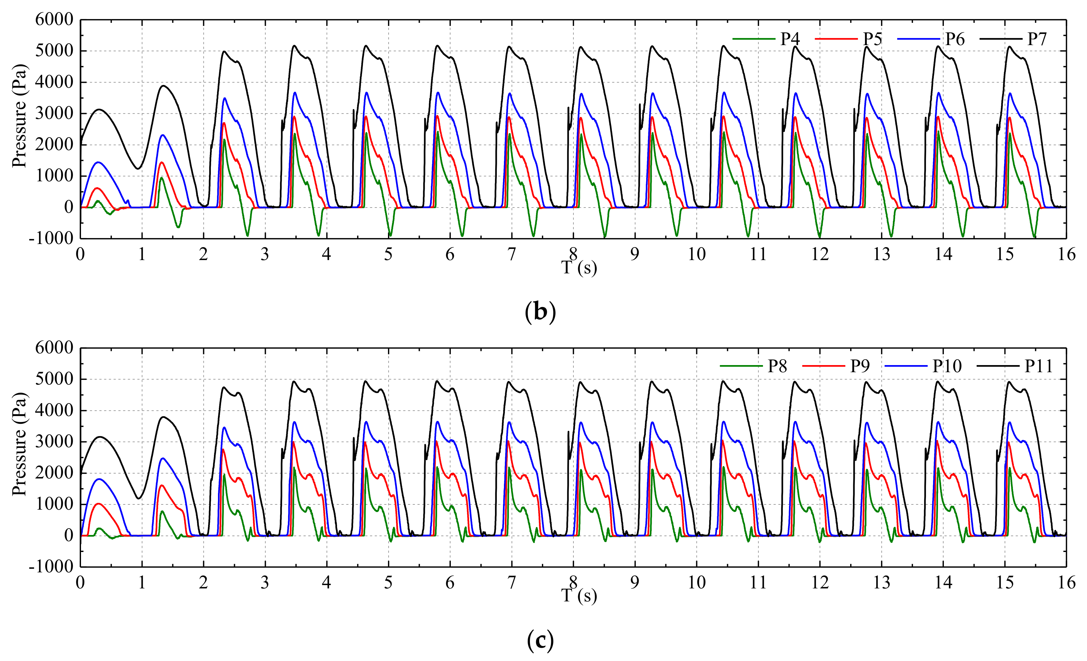
The time series of ship bow impact pressure in the severest wave condition (λ/L = 1.2, wave heading 45°/315° and ship speed Fn = 0.25) is summarized in Figure 26. In the figure, only the pressure data on the port side and the centerline of bow are presented due to the symmetry of the ship motion response and pressure distribution. Generally, the peak value of impact pressure decreases from the bottom to the deck and also from the bow to the stern. For example, the pressure peak value decreases from P7 to P3 (or from P11 to P8) and also decreases from P1 to P8 (or from P2 to P9, from P3 to P10). The largest impact pressure peak occurred at pressure sensor P7, which is mounted on bow bottom area. The peak of the pressure signal is very sharp for the measurement in the upper locations, and the peak of the curve becomes much smoother for the measurement downward. This is affected by the contact time and velocity of the hull surface with respect to the water wave and the dead rise angle of geometry. The sharpness of the pressure signal increases with the increasing of velocity of water entry and with the decreasing of the dead rise angle.
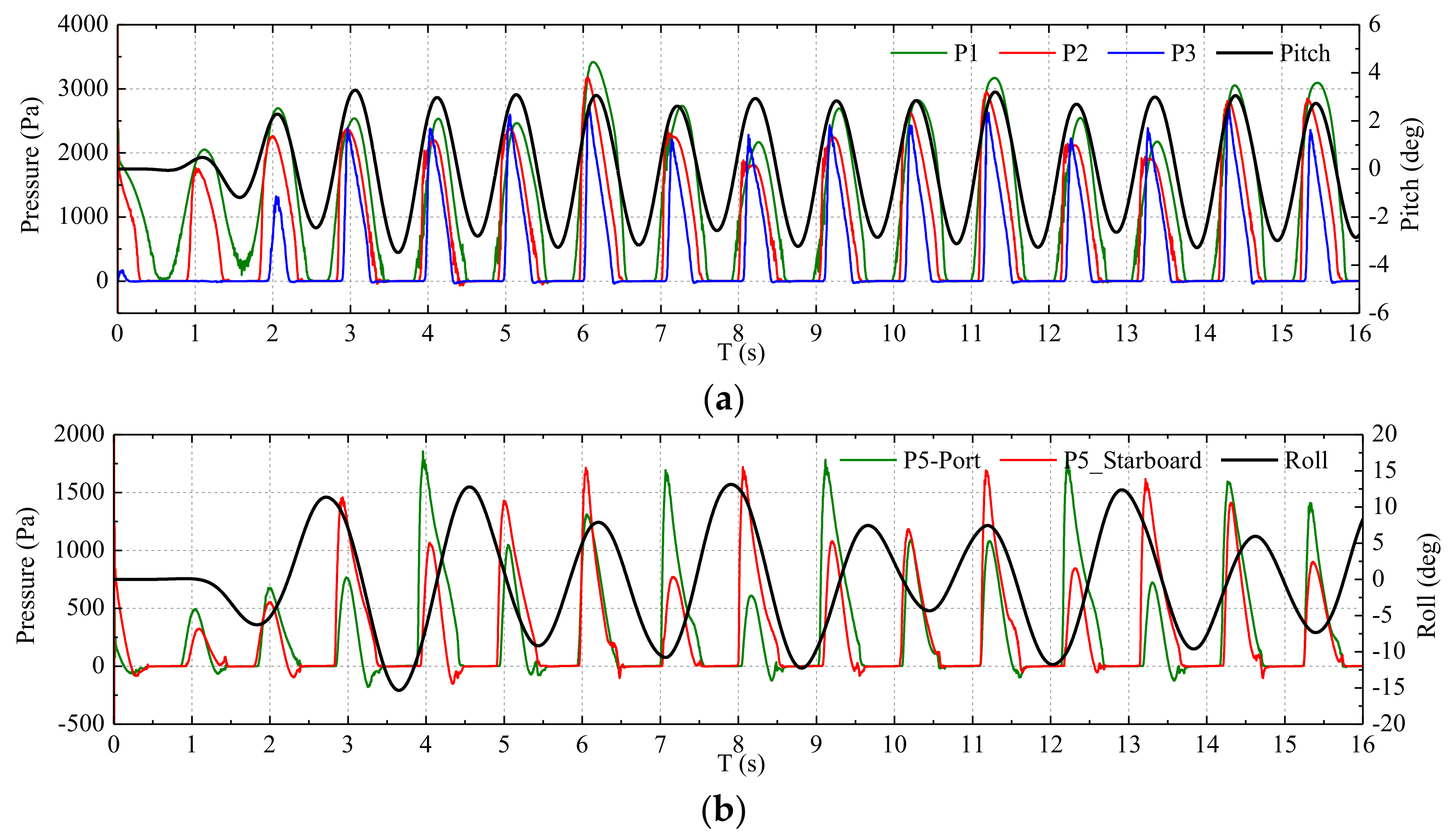
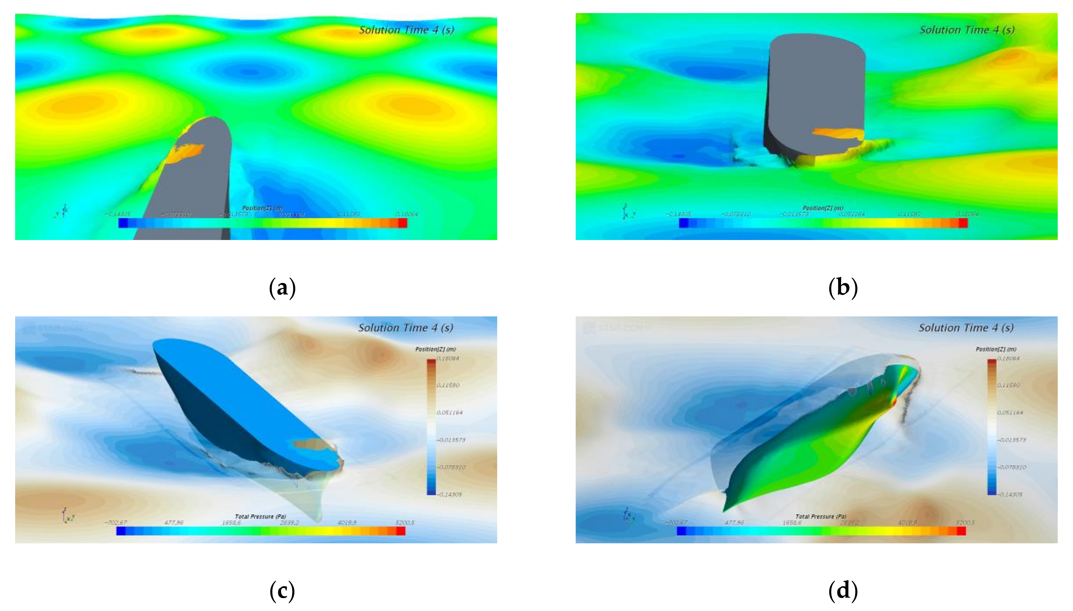
The asymmetric impact pressure acting on ship bow in the case of wave condition (λ/L = 1.2, wave heading 0°/90° and ship speed Fn = 0.25) is shown in Figure 27. Five typical pressure positions are involved for illustration, which include P1–P3 at centerline and two symmetric P5 points at both the port and starboard sides. The pitch and roll motion are also presented together with the pressure curves for reference. As seen from the results, the pressure peak for the measurements of P1–P3 at centerline occurred almost simultaneously when the ship was in a bow down motion phase. Their slamming peak values fluctuate in a small range. However, due to the large roll motion, the pressure signal P5 at the bow side area is unsteady, and the large peak value alternates between the port and starboard sides. Their slamming peak values fluctuate in a relatively large range. View of the ship wave interaction in the asymmetric wave field at t = 4 s from different visual angles are presented in Figure 28, which corresponds to the moment of largest impact peak at P5 of port side.
The largest peak values of slamming pressure monitored by different sensors in the two conditions are summarized in Table 4. It can be found that a small difference (below 1%) can be observed at the corresponding sensors of the port and starboard sides even in the symmetric wave 0° (45°/315°) case. This was caused by the error introduced in geometric modeling and grid generating and the strongly randomicity and uncertainty of the slamming signal. The peak pressure at each sensor positions in the symmetric wave 0° (45°/315°) case are all greater than in the asymmetric wave 45° (0°/90°) case. For ship sailing in the asymmetric wave 45° (0°/90°) case, the peak pressure on the starboard side are generally greater than the port side since the resultant wave heading is starboard quarter wave. For both of the two conditions, the largest impact pressure peak occurred at pressure sensor P7, which is mounted on bow bottom area, and the smallest pressure peak occurred at P8 due to its lowest velocity of water entry.
According to the above analysis, ship will probably encounter large amplitude vertical or transverse motion and severe slamming and green water on deck when sailing in cross waves. The cross wave will pose a threat to the navigational safety of a ship. Therefore, it is of great importance to provide some insightful strategies for the operational guidance of a ship when suffering a cross wave. As concluded from the wave analysis section, in the cross wave field, there exist stagnation lines where the wave elevation remains zero and time-invariant. The ship will experience the lowest wave if it travels along the stagnation lines. The motions of ship sailing along the stagnation line have been investigated in our recent work [24]. The lowest vertical motion responses can be realized when the ship sails along the stagnation lines at a wave heading of 0° (45°/315°).
6. Conclusions
This paper presents a numerical study on the seakeeping and slamming behavior of a S175 ship sailing in cross waves by CFD-based software STAR-CCM+. An URANS solver, which uses VOF and overset grid techniques, was developed in the framework of CFD to predict ship seakeeping behavior. This study also sheds some light on ship motion and slamming behavior in multi-directional or short-crested waves.
The numerical simulation results reveal that the cross wave can be approximately regarded as the linear superposition of two component regular waves. The surface elevation at a specific location within a monochromatic cross wave field follows the sine function with stagnation points existing in the wave field. The encounter wave is regular when the ship sails at a symmetrical wave heading with respect to the cross wave. However, the encounter wave is irregular and bi-chromatic when the ship sails at an asymmetrical wave heading with respect to the cross wave.
The ship heave and pitch motion is sinusoidal and regular, whereas the roll motion remains zero when the ship wave heading is symmetric with respect to the cross wave. The ship will experience the severest vertical motion when sailing at wave heading 45°/315°. The ship roll motion is generally large in addition to the pronounced vertical motions when the ship wave heading is asymmetric with respect to the cross wave. Ship vertical motion behavior in a cross wave is quite different from that in a regular wave, and the coupled effect of vertical and transverse motions of a ship in the cross wave should be of concern for the safety of ship.
For a ship advancing in a symmetric cross wave, the peak value of impact pressure decreases from the bottom to the deck and also from the bow to the aft. The peak of pressure signal is very sharp for the measurement in the upper locations, and the curve peak becomes much smoother for the measurement downwards. For ship advancing in an asymmetric cross wave, the pressure signal at bow side area is unsteady and the large peak value alternates between port and starboard sides due to the large roll motion.
Although the CFD model was preliminary validated by the experimental data of ship motion in uni-directional head regular wave from tank measurement, the tank experiments for ship operating in cross wave have not been conducted or reported. Future work will focus on the experimental investigation of ship motion behavior in a cross wave and the validation of the CFD numerical method using experiment data. Moreover, comprehensive analysis of ship motions and slamming loads in different cross waves (i.e., various wave lengths, wave heights, wave heading angles, and phase differences, and even bichromatic cross waves) will be undertaken in our future studies.
Author Contributions
J.J. and S.H. contributed equally to this paper. J.J. and S.H. designed the research scheme, S.H. conducted the CFD computation, J.J. analyzed the data, and J.J. wrote the paper. All authors have read and agreed to the published version of the manuscript.
Funding
This research was supported by the National Natural Science Foundation of China (No. 51909096), the Pre-Research Field Foundation of Equipment Development Department of China (No. 61402070106), and the Guangdong Basic and Applied Basic Research Foundation (No. 2020A1515011181).
Conflicts of Interest
The authors declare no conflict of interest. The funders had no role in the design of the study; in the collection, analyses, or interpretation of data; in the writing of the manuscript, or in the decision to publish the results.
References
- Zheng, W.T.; Miao, Q.M.; Zhou, D.C.; Kuang, X.F. Difference between motions in 3D and 2D waves. J. Ship Mech. 2009, 13, 184–188. (In Chinese) [Google Scholar]
- Hirdaris, S.E.; Bai, W.; Dessi, D.; Ergin, A.; Gu, X.; Hermundstad, O.A.; Huijsmans, R.; Iijima, K.; Nielsen, U.D.; Parunov, J.; et al. Loads for use in the design of ships and offshore structures. Ocean Eng. 2014, 78, 131–174. [Google Scholar] [CrossRef]
- Song, H.; Tao, L. Short-crested wave interaction with a concentric porous cylindrical structure. Appl. Ocean Res. 2007, 29, 199–209. [Google Scholar] [CrossRef] [Green Version]
- Ji, X.; Liu, S.; Bingham, H.B.; Li, J. Multi-directional random wave interaction with an array of cylinders. Ocean Eng. 2015, 110, 62–77. [Google Scholar] [CrossRef]
- Wang, L.Q. The Study of 3D and 3D Random Waves Acting on a Semicircular Breakwater. Ph.D. Thesis, Dalian University of Technology, Dalian, China, 2006. (In Chinese). [Google Scholar]
- Renaud, M.; Rezende, F.; Waals, O.; Chen, X.B.; Dijk, R.V. Second-order wave loads on a LNG carrier in multi-directional waves. In Proceedings of the ASME 27th International Conference on Offshore Mechanics and Arctic Engineering, Estoril, Portugal, 15–20 June 2008; pp. 1–8. [Google Scholar]
- Chen, J.P.; Wei, J.F.; Zhu, D.X. Numerical simulations of ship motions in long-crested and short-crested irregular waves by a 3D time domain method. Chin. J. Hydrodyn. 2011, 26, 589–596. (In Chinese) [Google Scholar]
- Jiao, J.; Chen, C.; Ren, H. A comprehensive study on ship motion and load responses in short-crested irregular waves. Int. J. Nav. Archit. Ocean Eng. 2019, 11, 364–379. [Google Scholar] [CrossRef]
- ITTC. The Seakeeping Committee, Final report and recommendations to the 26th ITTC. In Proceedings of the 26th ITTC, Vol. I, Rio de Janeiro, Brazil, 28 August–3 September 2011. [Google Scholar]
- ITTC. The Seakeeping Committee, Final report and recommendations to the 27th ITTC. In Proceedings of the 27th ITTC, Vol. I, Copenhagen, Denmark, 31 August–5 September 2014. [Google Scholar]
- ITTC. The Seakeeping Committee, Final Report and Recommendations to the 28th ITTC. In Proceedings of the 28th ITTC, Vol. I, Wuxi, China, 18–22 September 2017. [Google Scholar]
- Hashimoto, H.; Yoneda, S.; Omura, T.; Umeda, N.; Matsuda, A.; Stern, F.; Tahara, Y. CFD prediction of wave-induced forces on ships running in irregular stern quartering seas. Ocean Eng. 2020, 239, 106277. [Google Scholar] [CrossRef]
- Guo, B.J.; Steen, S.; Deng, G.B. Seakeeping prediction of KVLCC2 in head waves with RANS. Appl. Ocean Res. 2012, 35, 56–67. [Google Scholar] [CrossRef]
- Chen, S.; Hino, T.; Ma, N.; Gu, X. RANS investigation of influence of wave steepness on ship motions and added resistance in regular waves. J. Mar. Sci. Technol. 2018, 23, 991–1003. [Google Scholar] [CrossRef] [Green Version]
- Wang, W.; Bihs, H.; Kamath, A.; Arntsen, Ø.A. Multi-directional irregular wave modelling with CFD. Lecture Notes Civil Eng. 2019, 22, 521–529. [Google Scholar]
- Cao, H.J.; Wan, D.C. Development of multidirectional nonlinear numerical wave tank by Naoe-FOAM-SJTU solver. Int. J. Ocean Syst. Eng. 2014, 4, 49–56. [Google Scholar] [CrossRef]
- Wang, W.; Kamath, A.; Bihs, H. CFD simulations of multi-directional irregular wave interaction with a large cylinder. In Proceedings of the 37th International Conference on Ocean, Offshore and Arctic Engineering (OMAE), Madrid, Spain, 17–22 June 2018. [Google Scholar]
- Tezdogan, T.; Incecik, A.; Turan, O. Full-scale unsteady RANS simulations of vertical ship motions in shallow water. Ocean Eng. 2016, 123, 131–145. [Google Scholar] [CrossRef] [Green Version]
- Pereira, F.S.; Eça, L.; Vaz, G. Verification and Validation exercises for the flow around the KVLCC2 tanker at model and full-scale Reynolds numbers. Ocean Eng. 2017, 129, 133–148. [Google Scholar] [CrossRef]
- CD-adapco. User Guide STAR-CCM+ Version 14.02; CD-adapco: Melville, NY, USA, 2019. [Google Scholar]
- Li, D.Q.; Li, G.H.; Dai, J.J.; Zhang, Y.L.; Li, P. Numerical prediction of the added resistance and motions of ship in head waves based on overset mesh method. Ship Sci. Technol. 2018, 40, 13–20. (In Chinese) [Google Scholar]
- Huang, S.X.; Jiao, J.L.; Chen, C.H. Comparative study on ship motions in uni- and bi-directional waves by CFD. In Proceedings of the 30th International Ocean and Polar Engineering Conference (ISOPE-2020), Shanghai, China, 12–16 October 2020. [Google Scholar]
- Fonseca, N.; Guedes Soares, C. Experimental investigation of the nonlinear effects on the vertical motions and loads of a containership in regular waves. J. Ship Res. 2004, 48, 118–147. [Google Scholar]
- Jiao, J.L.; Huang, S.X.; Chen, C.H. Numerical investigation of ship motions in cross waves using CFD. Appl. Ocean Res. 2020. (Under Review). [Google Scholar]
Figure 1.
Phenomenon of cross sea wave: (a) swell wave; (b) wind wave.

Figure 2.
Body plan of the S175 hull.

Figure 3.
A 3D view of the model hull.

Figure 4.
Arrangement of pressure sensors.

Figure 5.
Overview of the fluid domain.

Figure 6.
General view of meshes in fluid domain.

Figure 7.
Refined grid near the free surface and hull.

Figure 8.
Boundary layer mesh around hull surface at bow and stern: (a) stern; (b) bow.

Figure 9.
Example of the simulated cross wave field.

Figure 10.
The initialized cross wave for different ship wave headings: (a) 45°/315° (Case 4); (b) 0°/90° (Case 9); (c) 45°/135° (Case 10); (d) 90°/180° (Case 11); (e) 135°/225° (Case 12).
Figure 10.
The initialized cross wave for different ship wave headings: (a) 45°/315° (Case 4); (b) 0°/90° (Case 9); (c) 45°/135° (Case 10); (d) 90°/180° (Case 11); (e) 135°/225° (Case 12).

Figure 11.
Surface elevation of ship encounter wave: (a) 45°/315° (Case 4); (b) 0°/90° (Case 9); (c) 45°/135° (Case 10); (d) 90°/180° (Case 11); (e) 135°/225° (Case 12).
Figure 11.
Surface elevation of ship encounter wave: (a) 45°/315° (Case 4); (b) 0°/90° (Case 9); (c) 45°/135° (Case 10); (d) 90°/180° (Case 11); (e) 135°/225° (Case 12).


Figure 12.
Frequency domain results of ship encounter wave.

Figure 13.
Wave components filtered from the measured cross wave: (a) 0°/90° (Case 9); (b) 45°/135° (Case 10); (c) 90°/180° (Case 11).
Figure 13.
Wave components filtered from the measured cross wave: (a) 0°/90° (Case 9); (b) 45°/135° (Case 10); (c) 90°/180° (Case 11).


Figure 14.
Numerical simulation of ship motion in head regular wave: (a) overview of initial state; (b) green water on deck.
Figure 14.
Numerical simulation of ship motion in head regular wave: (a) overview of initial state; (b) green water on deck.

Figure 15.
Comparison of experimental and numerical ship motions in head regular waves: (a) heave; (b) pitch.
Figure 15.
Comparison of experimental and numerical ship motions in head regular waves: (a) heave; (b) pitch.

Figure 16.
Time series of ship heave motion in different wave headings: (a) 45°/315° (Case 4); (b) 0°/90° (Case 9); (c) 45°/135° (Case 10); (d) 90°/180° (Case 11); (e) 135°/225° (Case 12).
Figure 16.
Time series of ship heave motion in different wave headings: (a) 45°/315° (Case 4); (b) 0°/90° (Case 9); (c) 45°/135° (Case 10); (d) 90°/180° (Case 11); (e) 135°/225° (Case 12).


Figure 17.
Time series of ship roll and pitch motions in different wave headings: (a) 45°/315° (Case 4); (b) 0°/90° (Case 9); (c) 45°/135° (Case 10); (d) 90°/180° (Case 11); (e) 135°/225° (Case 12).
Figure 17.
Time series of ship roll and pitch motions in different wave headings: (a) 45°/315° (Case 4); (b) 0°/90° (Case 9); (c) 45°/135° (Case 10); (d) 90°/180° (Case 11); (e) 135°/225° (Case 12).


Figure 18.
Response statistical values at different resultant wave heading: (a) heave; (b) pitch; (c) roll.
Figure 18.
Response statistical values at different resultant wave heading: (a) heave; (b) pitch; (c) roll.

Figure 19.
Comparative view of ship green water on deck at bow emergence and down phases: (a) 0° (45°/315°) at t = 9 s; (b) 0° (45°/315°) at t = 9.6 s; (c) 180° (135°/225°) at t = 7.5 s; (d) 180° (135°/225°) at t = 9 s.
Figure 19.
Comparative view of ship green water on deck at bow emergence and down phases: (a) 0° (45°/315°) at t = 9 s; (b) 0° (45°/315°) at t = 9.6 s; (c) 180° (135°/225°) at t = 7.5 s; (d) 180° (135°/225°) at t = 9 s.

Figure 20.
Ship large amplitude roll motion process at wave heading 90° (45°/135°): (a) t = 4 s; (b) t = 4.8 s; (c) t = 5.6 s; (d) t = 6.4 s.
Figure 20.
Ship large amplitude roll motion process at wave heading 90° (45°/135°): (a) t = 4 s; (b) t = 4.8 s; (c) t = 5.6 s; (d) t = 6.4 s.

Figure 21.
Time series of ship vertical motion at different wave lengths: (a) heave; (b) pitch.

Figure 22.
Ship vertical motion amplitude value at different wave lengths: (a) heave; (b) pitch.

Figure 23.
Green water on deck for ship in different wave length: (a) λ/L = 0.8; (b) λ/L = 1.2; (c) λ/L = 1.5; (d) λ/L = 2.0.
Figure 23.
Green water on deck for ship in different wave length: (a) λ/L = 0.8; (b) λ/L = 1.2; (c) λ/L = 1.5; (d) λ/L = 2.0.

Figure 24.
Front and deck view of wave impact and green water on deck (λ/L = 1.2): (a) front view (t = 5.2 s); (b) deck view (t = 5.2 s); (c) front view (t = 6.1 s); (d) deck view (t = 6.1 s).
Figure 24.
Front and deck view of wave impact and green water on deck (λ/L = 1.2): (a) front view (t = 5.2 s); (b) deck view (t = 5.2 s); (c) front view (t = 6.1 s); (d) deck view (t = 6.1 s).

Figure 25.
Starboard side view of wave impact and green water on deck (λ/L = 1.2): (a) top view (t = 5.2 s); (b) bottom view (t = 5.2 s); (c) top view (t = 6.1 s); (d) bottom view (t = 6.1 s).
Figure 25.
Starboard side view of wave impact and green water on deck (λ/L = 1.2): (a) top view (t = 5.2 s); (b) bottom view (t = 5.2 s); (c) top view (t = 6.1 s); (d) bottom view (t = 6.1 s).

Figure 26.
Impact pressure for the case of ship sail in symmetric wave field: (a) sensors at centerline of bow; (b) sensors at cross-section of #19.5 station; (c) sensors at cross-section of #19 station.
Figure 26.
Impact pressure for the case of ship sail in symmetric wave field: (a) sensors at centerline of bow; (b) sensors at cross-section of #19.5 station; (c) sensors at cross-section of #19 station.


Figure 27.
Impact pressure and pitch & roll for the case of ship sail in asymmetric wave field: (a) sensors at centerline of bow; (b) sensors at P5.
Figure 27.
Impact pressure and pitch & roll for the case of ship sail in asymmetric wave field: (a) sensors at centerline of bow; (b) sensors at P5.

Figure 28.
View of ship wave interaction in the asymmetric wave field (t = 4 s): (a) deck view; (b) front view; (c) top view; (d) bottom view.
Figure 28.
View of ship wave interaction in the asymmetric wave field (t = 4 s): (a) deck view; (b) front view; (c) top view; (d) bottom view.


Table 1.
Main properties of the S175 containership.
| Item | Full-Scale | Model |
|---|---|---|
| Scale | 1:1 | 1:40 |
| Length between perpendiculars (L) | 175 m | 4.375 m |
| Breadth (B) | 25.4 m | 0.635 m |
| Depth (D) | 19.5 m | 0.488 m |
| Draft (T) | 9.5 m | 0.238 m |
| Displacement (Δ) | 23,711 t | 370 kg |
| Block coefficient (CB) | 0.562 | 0.562 |
| Midship section coefficient (CM) | 0.990 | 0.990 |
| Prismatic coefficient (CP) | 0.568 | 0.568 |
| Longitudinal centre of gravity (LCG) from after perpendicular | 84.980 m | 2.125 m |
| Vertical centre of gravity (KG) from base line | 8.5 m | 0.213 m |
| Transverse radius of gyration | 9.652 m | 0.241 m |
| Longitudinal radius of gyration | 42.073 m | 1.052 m |
Table 2.
Numerical simulation conditions.
| Case ID | Wave Heading, β1/β2 (°) | Resultant Wave Heading β (°) | Wave length, λ/L | Wave Height, H (mm) | Phase Difference, ε (rad) | Ship Speed, Fn |
|---|---|---|---|---|---|---|
| 1−8 | 45/315 | 0 | 0.6, 0.8, 0.9, 1.0, 1.1, 1.2, 1.5, 2.0 | 120 | 0 | 0.25 |
| 9 | 0/90 | 45 | 1.0 | 120 | 0 | 0.25 |
| 10 | 45/135 | 90 | 1.0 | 120 | 0 | 0.25 |
| 11 | 90/180 | 135 | 1.0 | 120 | 0 | 0.25 |
| 12 | 135/225 | 180 | 1.0 | 120 | 0 | 0.25 |
Table 3.
Comparison of the peak frequency with encounter frequency.
| Wave Heading (°) | Peak Frequency (Hz) | Encounter Frequency (Hz) | Difference |
|---|---|---|---|
| 0 | 0.985 | 0.971 | 1.44% |
| 45/315 | 0.875 | 0.862 | 1.51% |
| 90 | 0.611 | 0.597 | 2.35% |
| 135/225 | 0.317 | 0.333 | 4.80% |
| 180 | 0.236 | 0.223 | 5.83% |
Table 4.
Summary of the largest peak values at bow area (in kPa).
| Sensor ID | P1 | P2 | P3 | P4 | P5 | P6 | P7 | P8 | P9 | P10 | P11 | |
|---|---|---|---|---|---|---|---|---|---|---|---|---|
| Symmetric case 0° (45°/315°) | Port | 4.40 | 4.49 | 4.75 | 2.41 | 2.92 | 3.68 | 5.17 | 2.18 | 3.03 | 3.65 | 4.94 |
| Starboard | 2.39 | 2.91 | 3.67 | 2.16 | 3.03 | 3.64 | ||||||
| Asymmetric case 45° (0°/90°) | Port | 2.72 | 3.18 | 3.42 | 1.51 | 1.84 | 2.56 | 3.89 | 1.42 | 1.97 | 2.56 | 3.79 |
| Starboard | 1.71 | 1.74 | 2.49 | 1.71 | 2.07 | 2.71 | ||||||
© 2020 by the authors. Licensee MDPI, Basel, Switzerland. This article is an open access article distributed under the terms and conditions of the Creative Commons Attribution (CC BY) license (http://creativecommons.org/licenses/by/4.0/).
Share and Cite
MDPI and ACS Style
Jiao, J.; Huang, S. CFD Simulation of Ship Seakeeping Performance and Slamming Loads in Bi-Directional Cross Wave. J. Mar. Sci. Eng. 2020, 8, 312. https://doi.org/10.3390/jmse8050312
AMA Style
Jiao J, Huang S. CFD Simulation of Ship Seakeeping Performance and Slamming Loads in Bi-Directional Cross Wave. Journal of Marine Science and Engineering. 2020; 8(5):312. https://doi.org/10.3390/jmse8050312
Chicago/Turabian StyleJiao, Jialong, and Songxing Huang. 2020. "CFD Simulation of Ship Seakeeping Performance and Slamming Loads in Bi-Directional Cross Wave" Journal of Marine Science and Engineering 8, no. 5: 312. https://doi.org/10.3390/jmse8050312
Note that from the first issue of 2016, this journal uses article numbers instead of page numbers. See further details here.