
Complete Coverage Path Planning of an Unmanned Surface Vehicle Based on a Complete Coverage Neural Network Algorithm


1
College of Harbor, Coastal and Offshore Engineering, Hohai University, Nanjing 210098, China
2
School of Naval Architecture, Ocean and Civil Engineering, Shanghai Jiao Tong University, Shanghai 200240, China
3
National Engineering Research Center of Dredging, Shanghai 200136, China
*
Author to whom correspondence should be addressed.
J. Mar. Sci. Eng. 2021, 9(11), 1163; https://doi.org/10.3390/jmse9111163
Submission received: 6 September 2021
/
Revised: 4 October 2021
/
Accepted: 11 October 2021
/
Published: 22 October 2021
(This article belongs to the Special Issue Advances in Autonomous Underwater Robotics Based on Machine Learning)
Abstract
:In practical applications, an unmanned surface vehicle (USV) generally employs a task of complete coverage path planning for exploration in a target area of interest. The biological inspired neural network (BINN) algorithm has been extensively employed in path planning of mobile robots, recently. In this paper, a complete coverage neural network (CCNN) algorithm for the path planning of a USV is proposed for the first time. By simplifying the calculation process of the neural activity, the CCNN algorithm can significantly reduce calculation time. To improve coverage efficiency and make the path more regular, the optimal next position decision formula combined with the covering direction term is established. The CCNN algorithm has increased moving directions of the path in grid maps, which in turn has further reduced turning-angles and makes the path smoother. Besides, an improved A* algorithm that can effectively decrease path turns is presented to escape the deadlock. Simulations are carried out in different environments in this work. The results show that the coverage path generated by the CCNN algorithm has less turning-angle accumulation, deadlocks, and calculation time. In addition, the CCNN algorithm is capable to maintain the covering direction and adapt to complex environments, while effectively escapes deadlocks. It is applicable for USVs to perform multiple engineering missions.
1. Introduction
The demand for the exploration and development of ocean coerce human beings to employ surface and underwater vehicles to explore and study water environments [1]. With the development of artificial intelligence, the unmanned surface vehicle (USV) has replaced human in certain fields to reduce cost and improve efficiency of exploration. Currently, USV has become a basic tool in marine exploration [2]. A USV refers to an intelligent platform that relies on shipborne sensors to navigate on the surface in an autonomous or semi-autonomous manner [3]. It is extensively employed in marine environment investigation, marine resources exploration, guard patrol, anti-mine, and anti-submarine missions [4].
The path planning of a USV implies that a USV selects an optimal or suboptimal obstacle avoidance path that can be connected from the starting point to the destination in the task area with reference to a certain index (such as the lowest work generation value, the shortest path length, and the shortest calculation time consumption) [5]. According to different planning purposes, the path planning can be categorized as point-to-point path planning and complete coverage path planning [6]. Point-to-point path planning is primarily used for the rapid movement of USVs in water environment. An optimal collision-free path from the origin to the destination is planned by the algorithm. Complete coverage path planning requires a USV to pass through every region of the workspace, and reduce repetition rate and turns of the path as much as possible [7]. In practical engineering applications, complete coverage path planning is often applied for the all-round search or information collection of the task area. Typical engineering applications include the use of USVs for terrain, velocity, water quality, and hydrological measurements [8].
Complete coverage path planning is extensively employed in the robotic navigation, such as the exact cell [9], boustrophedon cellular [10], morse [11], and line-sweep-based decompositions [12], etc. Traditional algorithms often plan paths according to fixed planning templates and are unable to dynamically adjust with environments, which is less smart. In a complex environment, the repetition rate will increase significantly. Recently, a neural network algorithm based on bionics is increasingly used in the field of complete coverage path planning for robotics. Yang [13] has proposed the biological inspired neural network (BINN) algorithm and applied it to the complete coverage path planning of cleaning robots. The BINN algorithm does not need any templates, even in unknown environments. And it’s capable of planning more reasonable and shorter collision-free complete coverage paths. However, the BINN algorithm has certain defects, such as a complex process of calculation that is time-consuming and easy path deviation. Many scholars have improved the BINN algorithm to solve these drawbacks. Guo and Balakrishnan [14] have realized the continuous steering control of the robot covering the bounded area in a limited time based on the biological excitation neural network. Fan et al. [15] have proposed an improved algorithm employing the template method for the possible local optimal solution of the BINN algorithm. Zhu et al. [16] have simplified the calculations of the shunting equation and proposed an improved algorithm based on the BINN algorithm for the AUV complete coverage path planning, which can effectively reduce the path planning time and improve the efficiency. Zhao et al. [17] have proposed a new optimal decision formula to solve the problem of the local path yaw, and applied it to the complete coverage path planning of USVs.
The BINN algorithm is mainly used for mobile robots on land (such as cleaning robots). When it is applied for a USV in water, due to the differences in the dynamics between a land robot and a USV, the BINN algorithm causes a series of problems, such as time-consuming, too many navigation direction changes, excessive turning-angles, and difficult to maintain a covering direction.
In this paper, with the aim of addressing the aforementioned problems, a complete coverage neural network (CCNN) algorithm is proposed for the path planning of a USV. The CCNN algorithm simplifies the differential equation for calculating the neural activity into a simple equation with the environmental correction term. An optimal next position decision formula combining with the covering direction term is established for the better selection of the next position. Also, compared with the BINN algorithm, the CCNN algorithm increases 4 more moving directions of the path in grid maps, which contributes to a smoother path. With the aid of the turn avoidance (TA) inspection, the continuous turns to avoid repetition are further reduced. Furthermore, an improved A* algorithm that adds turning cost into the heuristic function is introduced to escape deadlocks. As a consequence, the CCNN algorithm can generate a coverage path with a smaller turning-angle and fewer navigation direction changes in shorter calculation time, compared with the BINN algorithm. Also, it’s able to maintain a fixed covering direction and escape the deadlock effectively.
The rest of this paper is organized as follows. In Section 2, the principle and process of the CCNN algorithm is described in detail. In Section 3, simulations studies have been carried out to compare the effects of multiple algorithms in artificial and real-world environments. Finally, concluding remarks are summarized in Section 4.
2. Complete Coverage Neural Network (CCNN) Algorithm
2.1. The Dynamics Model of USV
In general, dynamics of a USV in 6 degrees of freedom (6 DOF) include surge, sway, heave, roll, pitch and yaw. However, the USV with dual-propeller propulsion system merely stresses the model of horizontal motion components in 3 degrees of freedom (3 DOF), including surge, sway, and yaw [18], as shown in Figure 1.
Suppose there is no side thruster on the USV, and effects of disturbance forces are not stressed for the sake of simplicity. The motion equation of the USV in 3 DOF can be described as follows [19]:
where is the matrix of inertia parameters. C(ν) is the Coriolis and centripetal matrix. is the matrix of hydrodynamic damping parameter. is the position vector of a USV in earth-fixed frame. is the velocity vector of a USV in body-fixed frame consisting of the velocities u in surge and v in sway, and yaw rate r. is the control vector, and are the surge force and the yaw torque input, respectively.
Compared with a USV, the dynamics model of a mobile robot on land (such as cleaning robot) does not have hydrodynamic damping term. It concludes ground friction and propulsion resistance as constraints term to the motion equation [20]. Since ground friction is much larger than hydrodynamic damping, a mobile robot on land can easily perform braking, turning in place, and other complex movements. However, it’s much more difficult for a USV to perform precise motion control. Especially in the presence of water currents, an excessively large turning-angle may cause the USV to be washed away by water currents, making it difficult to approach the scheduled path. Therefore, when conducting the complete coverage path planning of a USV, it’s better to reduce the turning-angle and navigation direction changes, maintain a certain covering direction, and fully consider the impact of the environment on the planning results.
2.2. Principle of the BINN Algorithm
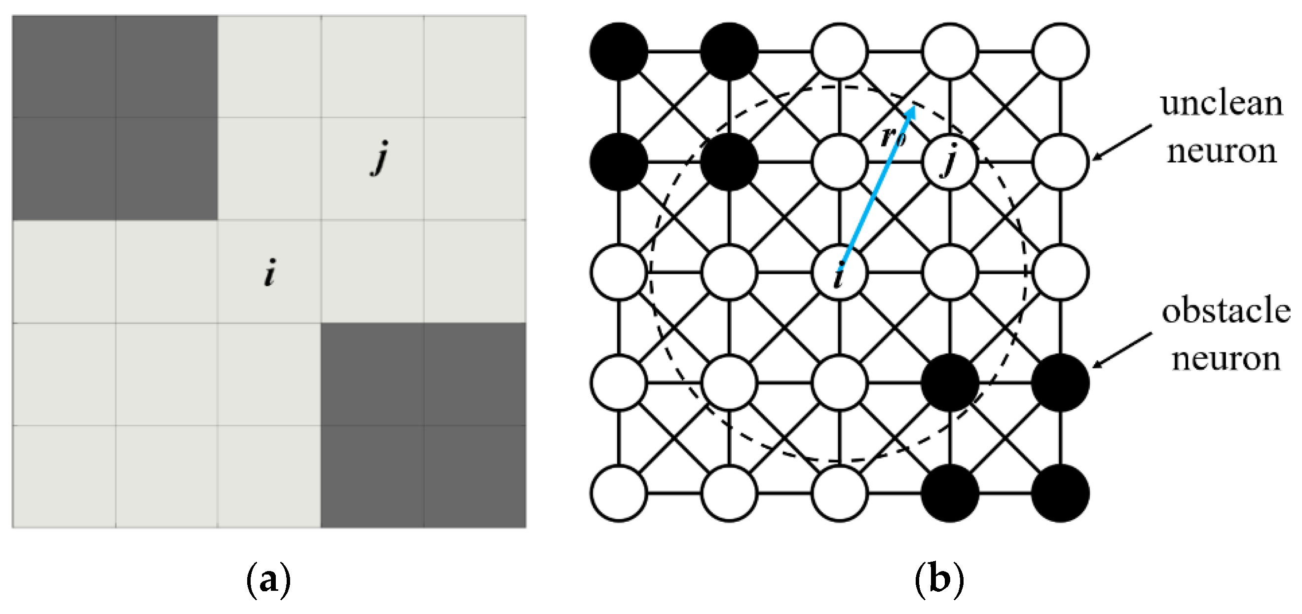
Hodgkin and Huxley [21] have proposed the circuit model of the nerve cell membrane and the dynamic equation describing the cell membrane (Hodgkin and Huxley model), Grossberg [22] has proposed the shunting equation based on the Hodgkin and Huxley model and applied it to biology and machine vision, sensing and motion control, and other fields. Based on the shunting equation proposed by Grossberg [22], Yang [13] has proposed the biologically inspired neural network (BINN) algorithm and applied it to the complete coverage path planning of mobile robots, and achieved good results. It should be noted that while the BINN method is called neural network, it has significant differences from the traditional neural networks. The traditional neural network often contains the input layer, output layer, hidden layer, and neuronal transfer function. For the BINN, there is no such function [16]. The idea of the BINN model is to consider the dynamically changing environment as a neural network architecture with dynamic neural activity. Neurons are divided into unclean, cleaned, and obstacle neurons in the network, as shown in Figure 2. The unclean neurons will attract the robot in the whole workspace, while the obstacle neurons have local effect to avoid collisions. The collision-free path of a mobile robot is planned in real time based on the dynamic activity of each neuron in the neural network.
The shunting equation proposed by Grossberg [22] has the following form:
where represents the activity of the ith neuron. Here A represents the attenuation rate, B and D represent the upper and lower limits of the neural activity, respectively. Here k is the number of neurons adjacent to the ith neuron. is the external input, which can be defined as:
where E is a very large positive constant. The terms and are the excitatory and inhibitory inputs, respectively. Function is the Relu function defined as , and . represents the connection weight for the ith and the jth neurons, which can be defined as:
where is the neuron connection radius, which is related to the detection range of the robot. And represents the Euclidean distance between the ith and the jth neuron.
Further, for the complete coverage path planning of mobile robots, navigation direction changes should be avoided as much as possible. Yang [23] has proposed a next position decision formula to optimize the selection of the next position. For the given current robot position , the next position is obtained by
where the current position is , the previous position is , and the next position is . c is a positive constant and k is the number of neighboring neurons of the th neuron, i.e., all the possible next positions of the current position . Variable is the neural activity of the jth neuron that is the same as that in Equation (3). is a monotonically increasing function of the difference between the current to next robot moving directions. is the turning-angle between the current moving direction and next moving direction. Here, atan2 indicates the function used to calculate the four-quadrant inverse tangent of fixed-point values in C language, which can be defined as:
While the robot is planning the coverage path, the activities of neurons with different attributes change over time, as shown in Figure 3a. Then the robot uses the next position decision formula to select the next waypoint until it covers all neurons. As shown in Figure 3b, , , according to the next position decision formula, (4,5) is the next waypoint. In Figure 3b, the dark gray grid represents the obstacle neuron, the white grid represents the unclean neuron, the dark green grid represents the cleaned neuron, and the green grid S represents the starting point. The dashed line indicates the generated path.
2.3. Principle of the CCNN Algorithm
The BINN algorithm is a complete coverage path planning method mainly used for indoor cleaning robots. A cleaning robot is easy to operate, the BINN algorithm does not need to consider the robot’s dynamics. However, as mentioned above, the dynamics of a USV is quite different from that of a cleaning robot. When it plans a coverage path for a USV, a series of problems will arise, such as easy path deviation, hard to maintain the covering direction, and low adaptability to complex environment, etc. To solve these problems and improve the effectiveness, inspired by the principle of the BINN algorithm, a CCNN algorithm for complete coverage path planning of the USV has been proposed in this paper. The basic idea in CCNN algorithm of environment modeling and neural activity calculation is the same as BINN algorithm. The main improvements of the CCNN algorithm lie in the calculation process of neural activity, the next position decision formula and the moving directions of the path.
The neural activity calculation formula employed in the CCNN algorithm is given as:
where represents the activity of the ith neuron. represents the attribute of the ith neuron, defined as:
where a is the upper limit of neural activity.
In Equation (10), is the environmental correction term and k is the number of neighboring neurons of the jth neuron. represents the Euclidean distance between the ith neuron and the jth neuron. Further, represents the gain coefficient of the environmental correction term, defined as:
where is the gain coefficient of the unclean neurons, the gain coefficient of the cleaned neurons and the gain coefficient of the obstacle neurons.
The next position decision formula is optimized as:
where the current position is , the previous position is , and the next position is . Here , . is the covering direction, up is (0,−1), down is (0,1), left is (−1,0), right is (1,0), upper left is (−1,−1), and lower left is (−1,1), the upper right is (1,−1), the lower right is (1,1). Further, c is the gain coefficient of the covering direction term, and b is a positive constant, viz., . represents the included angle between the current direction and the previous direction, viz., . represents the included angle between the current direction and the covering direction, viz., .
2.3.1. Improve on the Calculation Process of Neural Activity
The BINN algorithm calculates the neural activity by solving ordinary differential equation Equation (3). For the cleaned neuron, the initial value is the activity of the unclean neuron at the current moment. Because the activity of the unclean neuron changes with time, the initial conditions of cleaned neurons are different. So, the calculation equation of each cleaned neuron is different. As shown in Figure 4, the time for the robot to pass through a grid is 0.01 s; 3 cleaned neurons will produce 3 different activity change curves. With the expansion of the path, the number of equations to be solved increases linearly, consuming a lot of computing resources, resulting in long calculation time.
The CCNN algorithm adopts a simplified neural activity calculation formula fused with environmental correction term (Equation (10)). It has avoided the computational complexity caused by solving differential equations, and effectively reduced calculation time. In a 10 × 10 grid map with no obstacles, the calculation time of the BINN algorithm is 68 times that of the CCNN algorithm, as shown in Figure 5 and Table 1. The environmental correction term reflects the influence of different neurons on the planning path. The gain coefficients of different neurons can be modified to adapt to the different environments, making the planned path more regular.
2.3.2. Improve on the Next Position Decision Formula
In the next position decision formula of BINN algorithm, the four-quadrant inverse tangent function atan2 is used to calculate the included angle between the current moving direction and the next moving direction (Equation (8)). The path will be biased to the left and down. Therefore, the next position decision formula of BINN algorithm is only suitable for the ideal situation where the starting point is in the upper left corner. When the starting point is in the lower right corner, the planned path deviation will occur, resulting in multiple turns and reducing the coverage efficiency, as shown in Figure 6a.
The CCNN algorithm optimizes the next position decision formula by encapsulating the covering direction term. In Equation (14), reflects the included angle between the current direction and the previous direction. Compared with the function atan2 in the BINN algorithm, function arccos does not consider the absolute direction. It calculates the relative included angle only, which improves the applicability in different environments. Further, reflects the included angle between the current direction and the covering direction. When the included angle is smaller, the covering direction can be better maintained. Through the function sin, the influence of the direction can be eliminated and a more regular coverage planning path can be obtained, as shown in Figure 6.
2.3.3. Improve on the Moving Directions
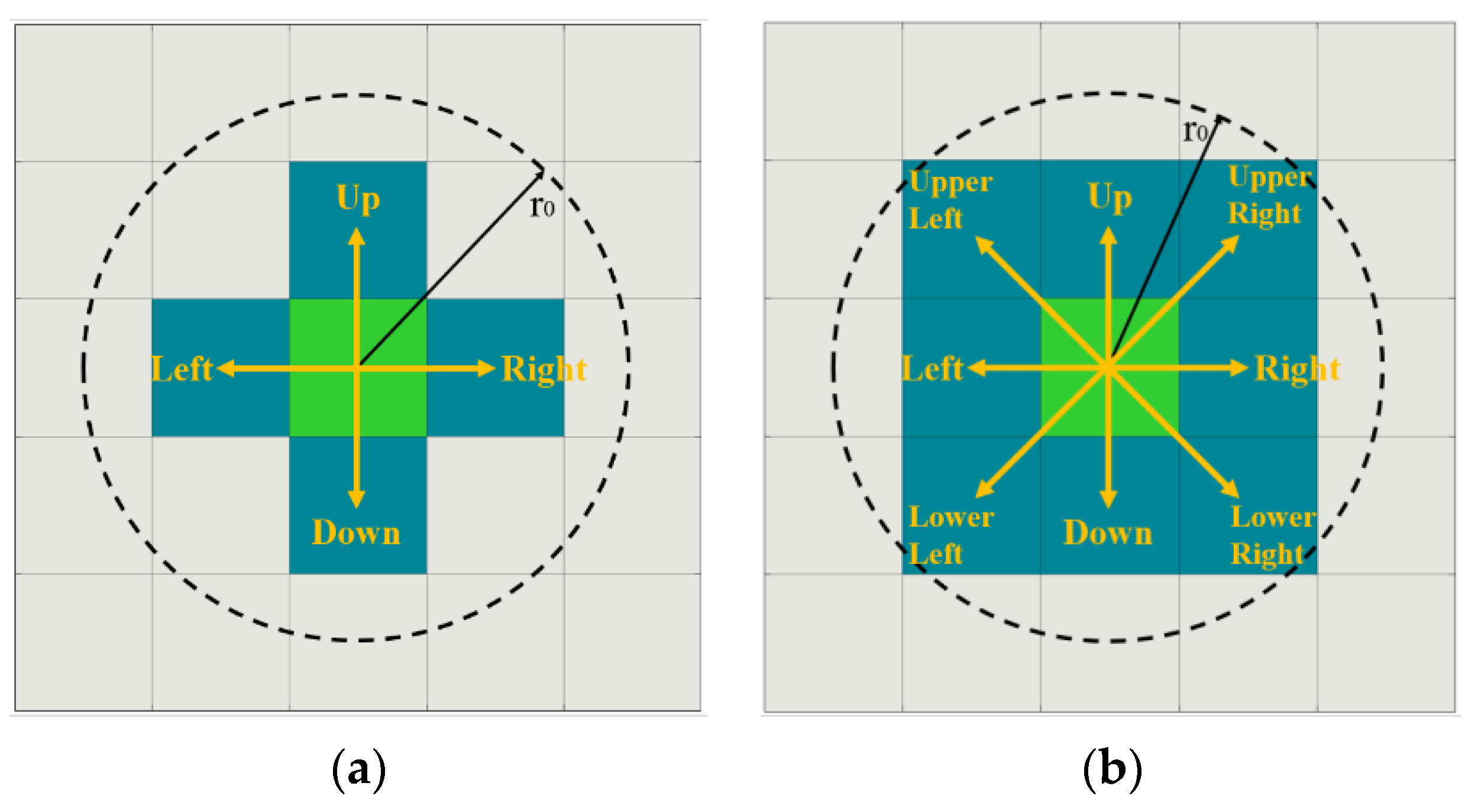
The activity of the unclean neuron in BINN algorithm are much higher than those of the cleaned neurons and obstacle neurons. Therefore, the path often shifts towards the area with more unclean neurons. Further, the next position decision formula of BINN algorithm only considers the included angle with the previous direction. At the edge of the map, the path is in danger of a yaw from the covering direction. Therefore, the moving directions of path in BINN algorithm is limited to only four, i.e., up, down, left, and right. The USV can only make a 90° turn, as shown in Figure 7a. For a USV, larger turning-angle and more navigation direction changes will make it difficult to track the planned path and will affect the operation results. With the aid of the environmental correction term and the covering direction term, the CCNN algorithm can solve the problem of easy yaw at the corner of the edge. It can increase the moving directions to eight, i.e., up, down, left, right, upper left, lower left, upper right, and lower right. As a result, the USV can make 45° and 90° turns, as shown in Figure 7b, which has reduced the turning-angle effectively.
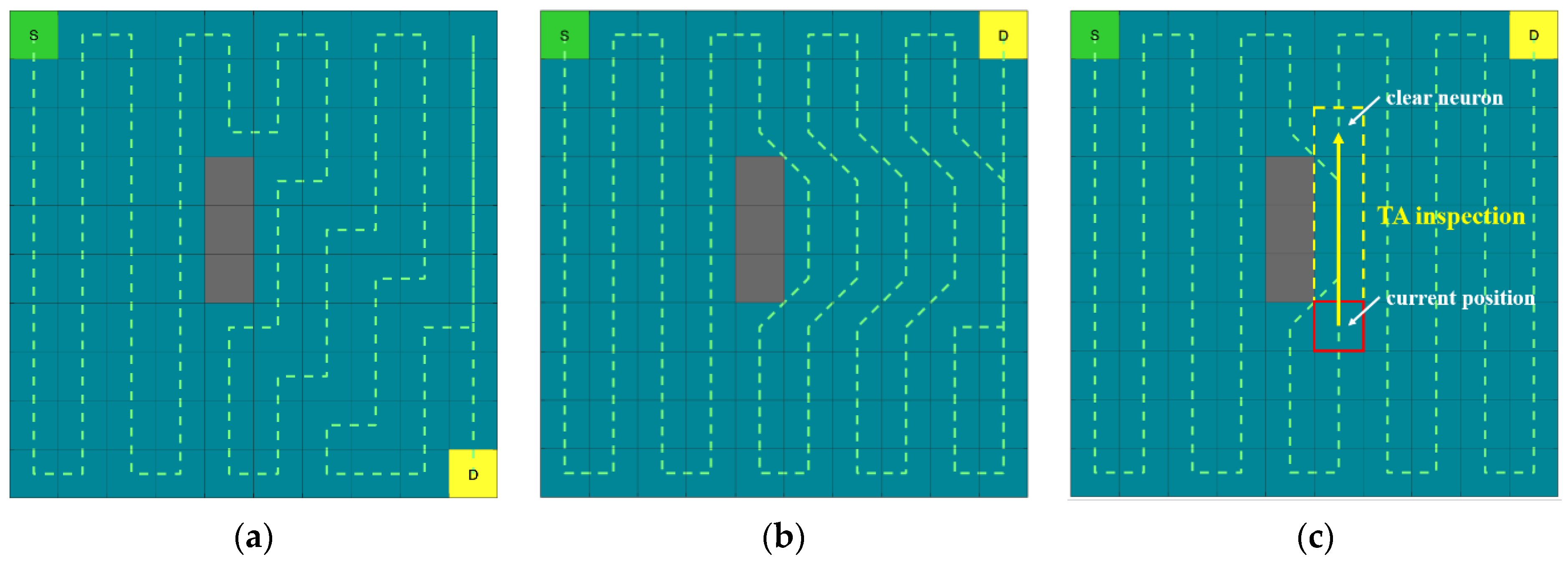
When the path come across the obstacle neurons, the BINN algorithm will deviate from the original covering direction and produce more turns, as shown in Figure 8a. Under the same circumstance, the CCNN algorithm will plan an obstacle avoidance path, and return to the original coverage path to continue scanning after bypassing the obstacle neurons. However, owing to the low activities of the cleaned neurons, the path will bypass the cleaned neurons to avoid repeated scanning, resulting in the continuous turns of the subsequent path, as shown in Figure 8b. Therefore, the turning avoidance (TA) inspection has been introduced to solve this problem. Once a cleaned neuron appears in front of the current position and the USV is about to take a turn, the TA inspection is performed to scan the neurons in the forward direction. If there are unclean neurons and no obstacle neurons in the inspection range, the path will avoid a turn and cross the front cleaned neurons to reach the unclean neurons and continue covering the remaining task area, as shown in Figure 8c. Otherwise, the path will take a turn to bypass the cleaned neuron. Although the repetition rate increases, the navigation direction changes decrease, and the covering direction is maintained.
2.4. Deadlock Escape Strategy Based on Improved A* Algorithm
A deadlock situation of a USV is the fact that the neighboring neuron of the central neuron is either visited, obstacle, or with smaller neural activity. An improved A* algorithm has been adopted to escape the deadlock in this paper. When the path falls into the deadlock, the algorithm will look for the unclean neuron, closest to the deadlock, as the escape point and automatically plan the path to the escape point, through the improved A* algorithm, to escape the deadlock.
The A* algorithm is a classical heuristic algorithm, which plans the optimal path through the heuristic function. The algorithm expands from the starting point to the neighboring area, and it calculates the cost value of each of the expand point and selects the expand point with the lowest cost value as the next point of the path. This process is repeated until the goal point is reached and the final path is generated. The heuristic function of A* algorithm is given as:
where is the total cost at the current point n, the moving cost from the starting point s to current point n, and the estimated path cost from the current point n to the goal point g, which is generally calculated in the following ways.
When mobile points can move up, down, left, and right, h(n) can be calculated using Manhattan distance formula:
The mobile points can move up, down, left, right, top left, top right, bottom left, and bottom right. The Chebyshev distance formula can be used here. The moving cost for the up, down, left, and right motion is 1, whereas the moving cost for the upper left, upper right, lower left, and lower right is the diagonal distance .
Generally, it is favorable to have less navigation direction changes. However, the heuristic function in A* algorithm only considers the path length, resulting in larger turning-angle and less smooth path, which makes it difficult for the navigation and path tracking control of a USV. Therefore, an improved A* algorithm has been proposed in this paper with respect to the dynamics characteristics of a USV and the shortage of excessive turns of A* algorithm, by adding the cost of the turning-angle to the heuristic function, the number of turns in the path has been reduced. The path with the smallest turning-angle accumulation and the shortest path length is selected as the optimal path. The improved function is given as
where is the vector from the parent point p to the current point n. Further, is the vector from the grandparent point pp to the parent point p. represents the conversion ratio of the turning-angle and is the moving cost from the parent point p to the current point n. The cost of moving up, down, left, and right is one, and the cost of moving upper left, upper right, lower left, and lower right is √2.
To compare the effects of path planning between A* and improved A* algorithms, the simulation environment is set to 20 × 40 grid map and four vertical obstacles have been arranged along the horizontal direction in the environment. The generated path and the results from simulation are shown in Figure 9 and Table 2.
According to Figure 9 and Table 2, the A* algorithm generates the largest number of turns, though it can obtain a shorter path in a complex environment, thus resulting in a large turning-angle accumulation. Compared with the A* algorithm, the number of turns and turning-angle accumulation have been greatly reduced in the improved A* algorithm despite the increase in path length. The effect of is more significant than that of for an improved A* algorithm with different conversion ratios for the turning-angle. The number of turns and the turning-angle accumulation have been further reduced. Compared with the A* algorithm, the reduction in the number of turns and the turning-angle accumulation are 71.0% and 84.6%, respectively, in the improved A* algorithm with . For different environments, the path can be more suitable for the USV by changing conversion ratio of the turning-angle .
The generated path of the escaping the deadlock using the improved A* algorithm is shown in Figure 10. The red grid in the figure indicates the deadlock.
2.5. CCNN Algorithm Flow
The flow of the CCNN algorithm by integrating the improved A* algorithm to escape the deadlock is given as follows:
Initialize the map, rasterize the map information, set the unit grid as the scanning width of the USV, and assign the initial attributes to each neuron (obstacle, unclean, cleaned).
Parameter initialization: by setting the parameters a, b, c, , , and , besides setting the trend direction of the coverage path.
Entering the algorithm for pathfinding cycle: first check for the unclean neurons remaining in the map. If there are unclean neurons, further judge the deadlock. If there are no deadlocks, traverse the neurons around the current position and calculate the neural activity. The neuron with the largest neural activity is selected as the next position. If there are cleaned neurons in front of the path, the TA inspection is performed. If there are unclean neurons in the inspection range, the unclean neuron will be selected as the next position, or else it will remain unchanged.
If all neurons have been cleaned, the algorithm completes the jump out cycle. If it enters the deadlock, the improved A* algorithm will be used to escape the deadlock.
Subsequent to jumping out of the cycle, the planning path quality is evaluated. The repetitive rate, path length, turning-angle accumulation, and other relevant data are calculated.
The flow of the CCNN algorithm is shown in Figure 11.
3. Simulation Studies
In order to demonstrate the feasibility and efficiency of the proposed complete coverage path planning scheme based on CCNN algorithm, several path planning simulation studies are conducted in various environments, i.e., artificial environment and real-world environment. In this section, boustrophedon cellular [10], BINN [23], improved BINN [17] algorithm are compared to the CCNN algorithm. All simulations are performed in a PC with Intel i7 2.2 GHz and 16 GB RAM, running by the Visual Studio 2019 Community, Microsoft in USA.
3.1. Simulation in an Artificial Environment
The artificial environment is set to 15 × 30 grid map with concave obstacles, edge obstacles, jagged obstacles, etc. To verify the path planning effect of different algorithm in an artificial environment, the following simulation has been carried out:
The parameters of BINN algorithm are set as, viz., A = 10, B = D = 1, E = 100, μ = 1, and = 2. The BINN and improved BINN algorithms adopt the improved A* algorithm of the Manhattan distance formula with 4 directions of motion to escape the deadlock.
The parameters of the CCNN algorithm are set as a = 1.5, b = 0.5, c = 1, = 0.1, = 2, and = 2. The CCNN algorithm adopts the improved A* algorithm of the Chebyshev distance formula with 8 directions of motion to escape the deadlock.
The generated path and the simulation results of different algorithms are shown in Figure 12 and Table 3. The dark gray grid represents the obstacle neuron, the dark green grid represents the cleaned neuron, the green grid S represents the starting point, the yellow grid D represents the destination, and the red grid represents the deadlock. The dashed line indicates the generated path.
According to Table 3, it can be observed that the boustrophedon cellular algorithm obtains a complete coverage path using the longest path length and the most deadlocks, while the BINN algorithm effectively reduces the number of deadlocks and further shortens the path length. It should be noted that the improved BINNN algorithm generates the shortest path and the least repetitive rate. However, as shown in Table 3, the improved BINNN algorithm has the maximum turning-angle accumulation and the longest calculation time, which increases the difficulty of path tracking and reduces the efficiency of the algorithm. Comparing to the boustrophedon cellular, BINN, and improved BINNN algorithm, the CCNN algorithm generates a coverage path with the minimum turning-angle accumulation in the shortest calculation time and greatly reduces the number of deadlocks. When compared with other three algorithms, the turning-angle accumulation of CCNN algorithm has reduced by 4.0%, 5.2%, and 12.5% respectively, the calculation time has reduced by 39.9%, 98.6% and 98.6% respectively. Therefore, the CCNN algorithm can find a nearly shortest and the least navigation direction changes path using the shortest time.
More practically, as shown in Figure 12, with the aid of the environmental correction term and 8 moving directions of the path in grid maps, the path generated by the CCNN algorithm can produce fewer turns near jagged obstacles and concave obstacles. Besides, by the optimal next position decision formula combining with the covering direction term, the CCNN algorithm maintains a consistent overall covering direction. However, the boustrophedon, BINN, and improved BINNN algorithms produce more turns near various obstacles, and the covering direction is not regular enough. Clearly, the CCNN algorithm can better adapt to complex environments and maintain a certain covering direction.
3.2. Simulation in a Real-World Environment
When a USV performs operational tasks, it needs to rely on the online satellite map or the electronic ocean map for path planning. A real-world environment is more complex than an artificial environment. The distribution of size and location of obstacles are increasingly random, which will in turn influence the result of path planning. A 750 × 1500 m ocean area has been set up, where there are islands and shorelines of different sizes. The image of the real-world environment is shown in Figure 13.
To verify the path planning effect of different algorithms in a real-world environment, the following simulation has been carried out:
The parameters of the BINN algorithm have been set as, viz., A = 10, B = D = 1, E = 100, μ = 1, and = 2. The BINN and improved BINN algorithms adopt the improved A* algorithm of the Manhattan distance formula with 4 directions of motion to escape the deadlock.
The parameters of the CCNN algorithm are set as, viz., a = 1.5, b = 0.5, c = 1, = 0.4, = 2, and = 2. The CCNN algorithm adopts the improved A* algorithm of the Chebyshev distance formula with 8 directions of motion to escape the deadlock.
The generated path and simulation results are shown in Figure 14 and Table 4. The green grid S represents the starting point, the yellow grid D represents the destination, and the red grid represents the deadlock. The dashed line indicates the generated path.
According to Table 4, the CCNN algorithm plans the path with the least number of deadlocks within the shortest time. Although the path planned by the improved BINN algorithm is shorter with less repetitive rate (only 6.6% shorter than the CCNN), it has the maximum turning-angle accumulation and longer calculation time. While the path generated by the CCNN algorithm has the smallest turning-angle accumulation, which is reduced by 20.6%, 54.7%, and 61.3% respectively compared with the boustrophedon cellular, BINN, and improved BINN algorithm. In addition, the CCNN algorithm has the least deadlocks, which is reduced by 75.0%, 71.4%, and 50.0% respectively compared with the other 3 algorithms. Less navigation direction changes and deadlocks are more conducive for path tracking of a USV in a complex environment, which will greatly improve operation efficiency.
In the real-world environment, the covering direction is supposed to change with different terrain. As can be seen from Figure 14, the BINN algorithm does not consider the covering direction, the path is rather chaotic, which makes it difficult for a USV to navigate. Due to the limitation of the optimal decision formula, the improved BINN algorithm can only plan the path with vertical covering direction, resulting in a lot of turns. The boustrophedon cellular algorithm adopts horizontal covering direction, but it does not consider the specific environment, and plans the path with a fixed template, resulting in plenty of deadlocks and high repetition rate. The CCNN algorithm maintains horizontal covering direction in most positions. Through LOS inspection, although repetition rate increased slightly, continuous navigation direction changes are avoided, which is better for USV.
Finally, from Figure 12, Figure 13 and Figure 14 and Table 3 and Table 4, the CCNN algorithm enables a USV to avoid navigation direction changes and deadlocks as much as possible, and significantly reduces calculation time, which is conducive to the path tracking of USV. In this context, the proposed CCNN algorithm can efficiently carry out the complete coverage path planning of a USV.
4. Conclusions
In this paper, inspired by the principle of the BINN, a CCNN algorithm for complete coverage path planning of a USV is proposed for the first time. The CCNN algorithm provides a simplified calculation process of the neural activity and an optimal next position decision formula for path planning, which reflects the influence of the environment and covering direction on the planning results. It increases the moving directions of the path in grid maps and makes the path more flexible. An improved A* algorithm, which introduces turning cost into the heuristic function, is presented to escape deadlocks. The complete coverage path planning scheme for a USV based on the proposed algorithm is capable of autonomously planning a collision-free path that can not only significantly reduce the turning-angle accumulation, deadlocks, and calculation time, but also maintain the covering direction and adapt to complex environments. Simulations and comprehensive comparisons in artificial and real-world environments are conducted to demonstrate the feasibility and efficiency of the CCNN algorithm.
Author Contributions
Conceptualization, Y.-X.D. and J.-C.L.; methodology, Y.-X.D.; validation, P.-F.X., Y.-X.D. and J.-C.L.; formal analysis, Y.-X.D.; data curation, Y.-X.D.; writing—original draft preparation, Y.-X.D.; writing—review and editing, Y.-X.D.; supervision, P.-F.X.; project administration, P.-F.X.; funding acquisition, P.-F.X. All authors have read and agreed to the published version of the manuscript.
Funding
National Natural Science Foundation of China (52071131), Marine Science and Technology Innovation Project of Jiangsu Province (HY2018-15), and China Postdoctoral Science Foundation (2018M640390).
Institutional Review Board Statement
Not applicable.
Informed Consent Statement
Not applicable.
Data Availability Statement
Not applicable.
Acknowledgments
Thanks to Yan Kai, Chen Cheng and Hong-Xia Cheng for their preliminary preparations for this article.
Conflicts of Interest
The authors declare no conflict of interest.
References
- Xiang, X.; Yu, C.; Lapierre, L.; Zhang, J.; Zhang, Q. Survey on Fuzzy-Logic-Based Guidance and Control of Marine Surface Vehicles and Underwater Vehicles. Int. J. Fuzzy Syst. 2018, 20, 572–586. [Google Scholar] [CrossRef]
- Huntsberger, T.; Woodward, G. Intelligent Autonomy for Unmanned Surface and Underwater Vehicles. In Proceedings of the OCEANS’11 MTS/IEEE KONA, Waikoloa, HI, USA, 19–22 September 2011. [Google Scholar]
- Liu, Z.; Zhang, Y.; Yu, X.; Yuan, C. Unmanned surface vehicles: An overview of developments and challenges. Annu. Rev. Control. 2016, 41, 71–93. [Google Scholar] [CrossRef]
- Yan, R.-J.; Pang, S.; Sun, H.-B.; Pang, Y.-J. Development and missions of unmanned surface vehicle. J. Mar. Sci. Appl. 2010, 9, 451–457. [Google Scholar] [CrossRef]
- Li, J.; Sun, X.-X. Route planning’s method for unmanned aerial vehicles based on improved a-star algorithm. Binggong Xuebao Acta Armamentarii 2008, 29, 788–792. [Google Scholar]
- Yan, M.Z.; Zhu, D.Q. An Algorithm of Complete Coverage Path Planning for Autonomous Underwater Vehicles. Key Eng. Mater. 2011, 467–469, 1377–1385. [Google Scholar] [CrossRef]
- Enric, G.; Marc, C. A survey on coverage path planning for robotics. Robot. Auton. Syst. 2013, 61, 1258–1276. [Google Scholar]
- Wang, Y.; Han, Q. Network-Based Fault Detection Filter and Controller Coordinated Design for Unmanned Surface Vehicles in Network Environments. IEEE Trans. Ind. Inform. 2016, 12, 1753–1765. [Google Scholar] [CrossRef]
- Latomabe, J.C. Robot Motion Planning. Commun. Pure Appl. Math. 1991, 48, 1173–1186. [Google Scholar]
- Choset, H. Coverage Path Planning: The Boustrophedon Cellular Decomposition; Springer: London, UK, 1998. [Google Scholar]
- Acar, E.U.; Choset, H.; Rizzi, A.A.; Atkar, P.N.; Hull, D. Morse Decompositions for Coverage Tasks. Int. J. Robot. Res. 2002, 21, 331–344. [Google Scholar] [CrossRef]
- Huang, W.H. Optimal line-sweep-based decompositions for coverage algorithms. In Proceedings of the IEEE International Conference on Robotics and Automation, 2001 ICRA, Seoul, Korea, 21–26 May 2001; Volume 21, pp. 27–32. [Google Scholar]
- Luo, C.; Yang, S.X. A real-time cooperative sweeping strategy for multiple cleaning robots. In Proceedings of the 2000 IEEE International Symposium on Intelligent Control. Held Jointly with the 8th IEEE Mediterranean Conference on Control and Automation, Patras, Greece, 19 July 2000. [Google Scholar]
- Yi, G.; Balakrishnan, M. Complete coverage control for nonholonomic mobile robots in dynamic environments. In Proceedings of the IEEE International Conference on Robotics & Automation, Orlando, FL, USA, 15–19 May 2006. [Google Scholar]
- Fan, L.L.; Wang, Q.Z.; Sun, F.C. Simulation Research and Improvement on Biologically Inspired Neural Network Path Planning. J. Beijing Jiaotong Univ. 2006, 30, 84–88. (In Chinese) [Google Scholar]
- Zhu, D.; Tian, C.; Sun, B.; Luo, C. Complete Coverage Path Planning of Autonomous Underwater Vehicle Based on GBNN Algorithm. J. Intell. Robot. Syst. 2018, 94, 237–249. [Google Scholar] [CrossRef]
- Hong, Z.; Derun, Z.; Ning, W.; Chen, G. Research on Improved BINN Algorithm for Coverage of Prioritized Area in Path Planning of Unmanned Surface Vessel. Shipbuild. China 2020, 61, 91–102. (In Chinese) [Google Scholar]
- McCue, L. Handbook of Marine Craft Hydrodynamics and Motion Control [Bookshelf]. IEEE Control Syst. Mag. 2016, 36, 78–79. [Google Scholar] [CrossRef]
- Ma, Y.; Nie, Z.; Yu, Y.; Hu, S.; Peng, Z. Event-triggered fuzzy control of networked nonlinear underactuated unmanned surface vehicle. Ocean Eng. 2020, 213, 107540. [Google Scholar] [CrossRef]
- Karavaev, Y.L.; Kilin, A.A. The dynamics and control of a spherical robot with an internal omniwheel platform. Regul. Chaotic Dyn. 2015, 20, 134–152. [Google Scholar] [CrossRef]
- Hodgkin, A.L.; Huxley, A.F. A quantitative description of membrane current and its application to conduction and excitation in nerve. J. Physiol. 1952, 117, 500–544. [Google Scholar] [CrossRef] [PubMed]
- Öǧmen, H.; Gagné, S. Neural network architectures for motion perception and elementary motion detection in the fly visual system. Pergamon 1990, 3, 487–505. [Google Scholar] [CrossRef]
- Luo, C.; Yang, S.X. A Bioinspired Neural Network for Real-Time Concurrent Map Building and Complete Coverage Robot Navigation in Unknown Environments. IEEE Trans. Neural Netw. 2008, 19, 1279–1298. [Google Scholar] [CrossRef]
Figure 1.
Motions in 3 DOF of USV.

Figure 2.
A neural network based on a grid map in the BINN algorithm: (a) Grid Map. (b) Corresponding neural network.
Figure 2.
A neural network based on a grid map in the BINN algorithm: (a) Grid Map. (b) Corresponding neural network.

Figure 3.
The BINN algorithm path planning procedure: (a) The neural-activity landscape (b) Progress of selecting the next position.
Figure 3.
The BINN algorithm path planning procedure: (a) The neural-activity landscape (b) Progress of selecting the next position.

Figure 4.
Activities of different cleaned neurons in BINN algorithm: (a) Generated path. (b) Activities of different cleaned neurons.
Figure 4.
Activities of different cleaned neurons in BINN algorithm: (a) Generated path. (b) Activities of different cleaned neurons.

Figure 5.
Generated path in 10 × 10 grid map with no obstacles.

Figure 6.
Influence of the covering direction term on the generated path: (a) BINN algorithm. (b) CCNN algorithm without covering direction term. (c) CCNN algorithm with covering direction term.
Figure 6.
Influence of the covering direction term on the generated path: (a) BINN algorithm. (b) CCNN algorithm without covering direction term. (c) CCNN algorithm with covering direction term.

Figure 7.
Direction of motion of different algorithm: (a) BINN algorithm. (b) CCNN algorithm.

Figure 8.
Influence of the TA inspection on the generated path: (a) BINN algorithm. (b) CCNN algorithm without TA inspection. (c) CCNN algorithm with TA inspection.
Figure 8.
Influence of the TA inspection on the generated path: (a) BINN algorithm. (b) CCNN algorithm without TA inspection. (c) CCNN algorithm with TA inspection.

Figure 9.
Generated path of the A* algorithm and improved A* algorithm: (a) A* algorithm. (b) Improved A* algorithm with . (c) Improved A* algorithm with .
Figure 9.
Generated path of the A* algorithm and improved A* algorithm: (a) A* algorithm. (b) Improved A* algorithm with . (c) Improved A* algorithm with .

Figure 10.
Generated path of the escaping the deadlock using the improved A* algorithm.

Figure 11.
The flow of the CCNN algorithm.

Figure 12.
Generated path of different algorithms in the artificial environment: (a) Boustrophedon cellular algorithm. (b) BINN algorithm. (c) Improved BINN algorithm. (d) CCNN algorithm.
Figure 12.
Generated path of different algorithms in the artificial environment: (a) Boustrophedon cellular algorithm. (b) BINN algorithm. (c) Improved BINN algorithm. (d) CCNN algorithm.

Figure 13.
The real-world environment.

Figure 14.
Generated path of different algorithms in the real-world environment: (a) Boustrophedon cellular algorithm. (b) BINN algorithm. (c) Improved BINN algorithm. (d) CCNN algorithm.
Figure 14.
Generated path of different algorithms in the real-world environment: (a) Boustrophedon cellular algorithm. (b) BINN algorithm. (c) Improved BINN algorithm. (d) CCNN algorithm.


Table 1.
Calculation time in different algorithm.
| Algorithm | BINN | CCNN |
|---|---|---|
| Calculation time/s | 105.9 | 1.55 |
Table 2.
Simulation results of A* algorithm and improved A* algorithm.
| Algorithm | Path Length/Grid | Turning-Angle Accumulation/° | Number of Turns |
|---|---|---|---|
| A* | 40.3 | 585.0 | 7 |
| Improved A* | 41.9 | 135.0 | 3 |
| Improved A* | 41.9 | 90.0 | 2 |
Table 3.
Simulation results of different algorithms in artificial environment.
| Algorithm | Path Length/Grid | Turning-Angle Accumulation/° | Repetitive Rate/% | Number of Deadlocks | Calculation Time/s |
|---|---|---|---|---|---|
| Boustrophedon cellular | 457 | 8515 | 10.3 | 20 | 9.99 |
| BINN | 441 | 8640 | 16.0 | 14 | 414.9 |
| Improved BINN | 389 | 9360 | 4.9 | 3 | 423.6 |
| CCNN | 395 | 8190 | 5.3 | 3 | 6.0 |
Table 4.
Simulation results of different algorithms in the real-world environment.
| Algorithm | Path Length/km | Turning-Angle Accumulation/° | Repetitive Rate/% | Number of Deadlocks | Calculation Time/s |
|---|---|---|---|---|---|
| Boustrophedon cellular | 22.65 | 4877 | 8.0 | 8 | 6.2 |
| BINN | 20.85 | 8550 | 6.7 | 7 | 444.7 |
| Improved BINN | 19.85 | 9990 | 2.0 | 4 | 440.8 |
| CCNN | 21.25 | 3870 | 4.4 | 2 | 6.1 |
Publisher’s Note: MDPI stays neutral with regard to jurisdictional claims in published maps and institutional affiliations. |
© 2021 by the authors. Licensee MDPI, Basel, Switzerland. This article is an open access article distributed under the terms and conditions of the Creative Commons Attribution (CC BY) license (https://creativecommons.org/licenses/by/4.0/).
Share and Cite
MDPI and ACS Style
Xu, P.-F.; Ding, Y.-X.; Luo, J.-C. Complete Coverage Path Planning of an Unmanned Surface Vehicle Based on a Complete Coverage Neural Network Algorithm. J. Mar. Sci. Eng. 2021, 9, 1163. https://doi.org/10.3390/jmse9111163
AMA Style
Xu P-F, Ding Y-X, Luo J-C. Complete Coverage Path Planning of an Unmanned Surface Vehicle Based on a Complete Coverage Neural Network Algorithm. Journal of Marine Science and Engineering. 2021; 9(11):1163. https://doi.org/10.3390/jmse9111163
Chicago/Turabian StyleXu, Peng-Fei, Yan-Xu Ding, and Jia-Cheng Luo. 2021. "Complete Coverage Path Planning of an Unmanned Surface Vehicle Based on a Complete Coverage Neural Network Algorithm" Journal of Marine Science and Engineering 9, no. 11: 1163. https://doi.org/10.3390/jmse9111163
Note that from the first issue of 2016, this journal uses article numbers instead of page numbers. See further details here.