
A Wideband Radio Channel Sounder for Non-Stationary Channels: Design, Implementation and Testing


atlanTTic Research Center, University of Vigo, 36310 Vigo, Spain
*
Author to whom correspondence should be addressed.
Electronics 2021, 10(15), 1838; https://doi.org/10.3390/electronics10151838
Submission received: 30 June 2021
/
Revised: 22 July 2021
/
Accepted: 28 July 2021
/
Published: 30 July 2021
(This article belongs to the Special Issue Channel Measurements, Modelling and Simulations for Future Wireless Communication Systems)
Abstract
:The increasing bandwidths and frequencies proposed for new mobile communications give rise to new challenges for system designers. Channel sounding and channel characterization are important tasks to provide useful information for the design of systems, protocols, and techniques to fight the propagation impairments. In this paper, we present a novel radio channel sounder capable of dealing with non-stationary channels. It can be operated in real-time and has a compact size to ease transport. For versatility and cost purposes, the core of the system is implemented in Field Programmable Gate Arrays (FPGAs). Three measurement campaigns have been conducted to illustrate the performance of the sounder in both static and non-static channels. In its current configuration, the sounder reaches an RF null-to-null bandwidth of 1 GHz, providing a delay resolution of 2 ns, a maximum measurable Doppler shift of 7.63 kHz, and 4.29 s of continuous acquisition time. A comparison with other channel sounders in the literature reveals that our proposal achieves a good combination of performance, cost, and size.
1. Introduction
Wireless communications have been playing an increasing role in society since the 20th century. Electromagnetic spectrum is a scarce asset, so there has been a historical trend to use increasingly higher frequencies to allocate new communication systems. Larger bandwidths available at higher frequency bands, like the millimeter-wave (mmWave) band, enable larger data rates.
The need for channel characterization has made sounding an important field of knowledge. Through the use of sounders, it is possible to obtain different functions and figures of interest [1]. With these, predictions of how the channel will behave in the presence of different signals can be made. Channel models have been elaborated from the results of extensive sounding campaigns.
Taxonomically, channel sounders can be classified in two groups according to the channel characteristic functions and parameters they can measure: narrowband and wideband. Narrowband sounders are adequate for channels that behave in a correlated fashion within the bandwidth of interest. An unmodulated carrier can be used to fully characterize such channels and obtain fading characteristics and Doppler spread [2].
However, radio channel does not show a correlated behavior within the whole bandwidth of wideband systems. The symbol intervals are short compared to the delays of the different propagation paths produced by the scatterers present in the environment. This will produce inter-symbol interference (ISI) and limit the system throughput. In this case, wideband sounders are required to measure the channel impulse response (CIR) and the delay spread introduced by the channel. Alternatively, the frequency response of the channel or the coherence bandwidth can be measured. This parameter is defined as the bandwidth for which the channel exhibits a correlated behavior. The relation between delay spread and coherence bandwidth is assumed to be bound by Fleury’s limit [3].
Different techniques are used to extract wideband characteristics of the radio channel. We can thus divide wideband channel sounders between six different categories depending on how they measure the CIR:
- Impulse-train. The simplest idea for a wideband channel sounder, it consists in transmitting a very short pulse emulating a delta. At the receiver, the channel impulse response is directly obtained. This system is extremely sensitive to noise and interference. The other main drawback is that very short, high-energy pulses are hard to generate. Examples of this technique include [4,5].
- Swept time delay cross-correlation (STDCC). Based on the pulse-compression principle, it transmits a pseudorandom sequence. As the autocorrelation of such waveforms is a delta, the CIR is obtained by correlating the received signal with a copy of the transmitted one. Nonetheless, as a correlation requires the evaluation of all possible delay combinations between both sequences, STDCC sounders employ a slightly slower clock at reception. This way, one sequence slides over the other. Due to the pulse compression, a processing gain is achieved, enhancing dynamic range over the impulse-train sounder. Since the first use of this technique by Cox [6], it has been extensively employed in measurement campaigns [7,8,9,10,11,12]. This is due to the high bandwidth, dynamic range, and relative simplicity of these sounders. However, these sounders have a reduced channel sampling rate that limits the maximum tolerable Doppler shift.
- Convolution matched filter (CMF). Another way of implementing pulse compression, the matched filter provides a mean to compute correlation. Classic sounders of this type use surface acoustic wave (SAW) filters [13,14]. This allows operation in real time by eliminating the penalty on the channel-sampling rate imposed by STDCC. Nonetheless, SAW filters are hard to manufacture if the sequences are long. Implementing the filter in the digital domain instead is also impractical in these cases, at least to obtain real-time results.
- Offline correlation. In this case, the receiver samples and records the sounding signal. Correlation is then calculated offline. This method allows for an increase of the channel-sampling rate. However, this approach is demanding in terms of data storage speed and capacity. Often, expensive equipment, such as high-speed oscilloscopes, are used. Examples of this category include [15,16,17,18].
- Pulse compression-based sounders, which rely on chirp pulses to achieve bandwidth compression at baseband, may achieve faster probing rates [19].
- Frequency swept. In these sounders, the frequency of a tone is swept over the bandwidth of interest to directly obtain the frequency-transfer function of the channel. Usually, a vector network analyzer (VNA) is used to measure the scattering parameter S21 between transmission and reception. CIRs can be obtained by applying the inverse Fourier transform to the frequency response. Narrow sliding filters allow to achieve a great dynamic range. Nevertheless, the transmitter and receiver have to be directly connected and the slow swept requires the channel to remain stationary for a long time. Thereby, VNA-based sounders are typically used indoors and over short distances. As in the STDCC case, these sounders have been widely used [20,21,22,23].
- Multi-tone sounders. These sounders estimate the frequency response of the channel by transmitting a multi-tone signal like the one resulting from orthogonal frequency division multiplexing (OFDM). These kind of sounders operate quickly, and as such, many responses can be obtained per second [24]. Nonetheless, high sampling rates are required.
As stated before, the evolution of mobile communication systems requires increasing frequencies and bandwidths. Therefore, channel sounder capabilities have to keep improving to be able to provide useful data for channel characterization. Delay resolution has to keep up with the increasing bandwidths being used. Multiple sounders are capable of achieving delay resolutions in the order of a few nanoseconds. Nonetheless, other requisites arise, for example, mmWave channels may exhibit very low coherence times. This is the time interval during which the channel exhibits correlated behavior. The resolution in the time axis, i.e., the variation of the channel response with time, has to cope with these decreasing coherence times. As such, sounders that are capable of reaching high bandwidths with very short channel sampling periods are more required than ever.
The aim of this paper is to present a novel wideband channel sounder capable of dealing with non-stationary channels as well as to present some initial measurements in the 28.65 GHz band. It is based on the correlation of pseudorandom sequences, but the correlation is performed in the frequency domain. The sounder presents a good relation between performance and cost (<12.000 € for baseband components). It has a baseband bandwidth of 500 MHz, which enables a delay resolution of 2 ns, surpassing the maximum planned bandwidth of 400 MHz for the frequency range 2 (FR2) of the fifth generation (5G) of mobile communications [25]. In Section 2, the architecture of the developed sounding system is described. The procedures to conduct measurement campaigns are also explained. In Section 3, the results are exposed with brief explanations. A more thorough discussion is given in Section 4, which also compares the current sounder with other sounders from the literature.
2. Channel Sounder Design and Measurement Scenarios
As stated before, the channel sounder is based on the correlation properties of pseudorandom sequences. In contrast with STDCC or CMF sounders, both of which perform the correlation in the time domain, we compute the Fourier transform of the received signal in order to take advantage of the frequency domain properties. This way, the resource-expensive temporal convolution implied by the correlation becomes a less demanding product in the frequency domain. Thereby, we achieve the maximal measurement speed of the CMF sounders without dealing with highly complex SAW filters.
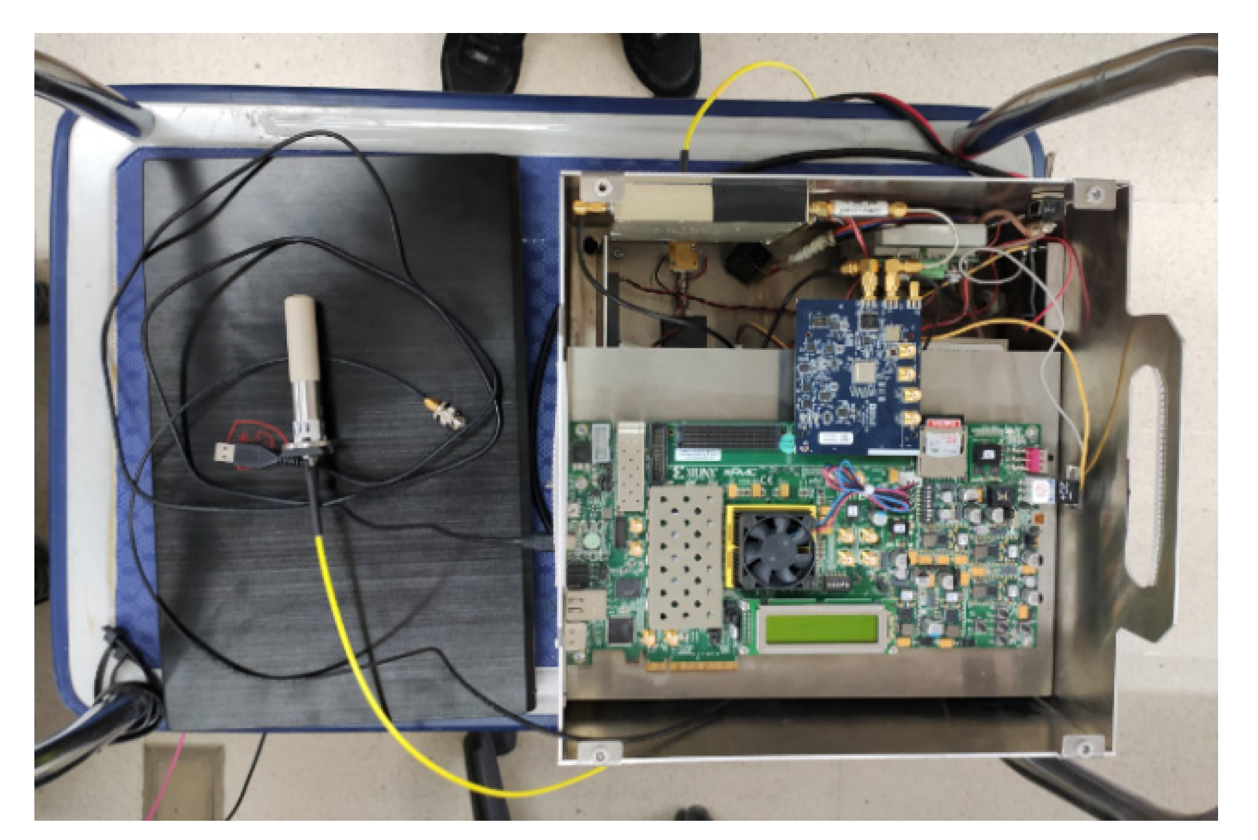
Both transmitter and receiver consist of frequency references, field-programmable gate arrays (FPGAs), converters, and RF frontends. They are shown in Figure 1 and Figure 2, respectively. In its current configuration, the bulkiness of the transmitter is significantly greater than that of the receiver. This is because the receiver is meant to be carried aboard a vehicle, meanwhile the transmitter is static, mimicking the behavior of a mobile communication’s system. In the following subsections, the configurations of the different parts of the sounder are described.
2.1. Transmitter
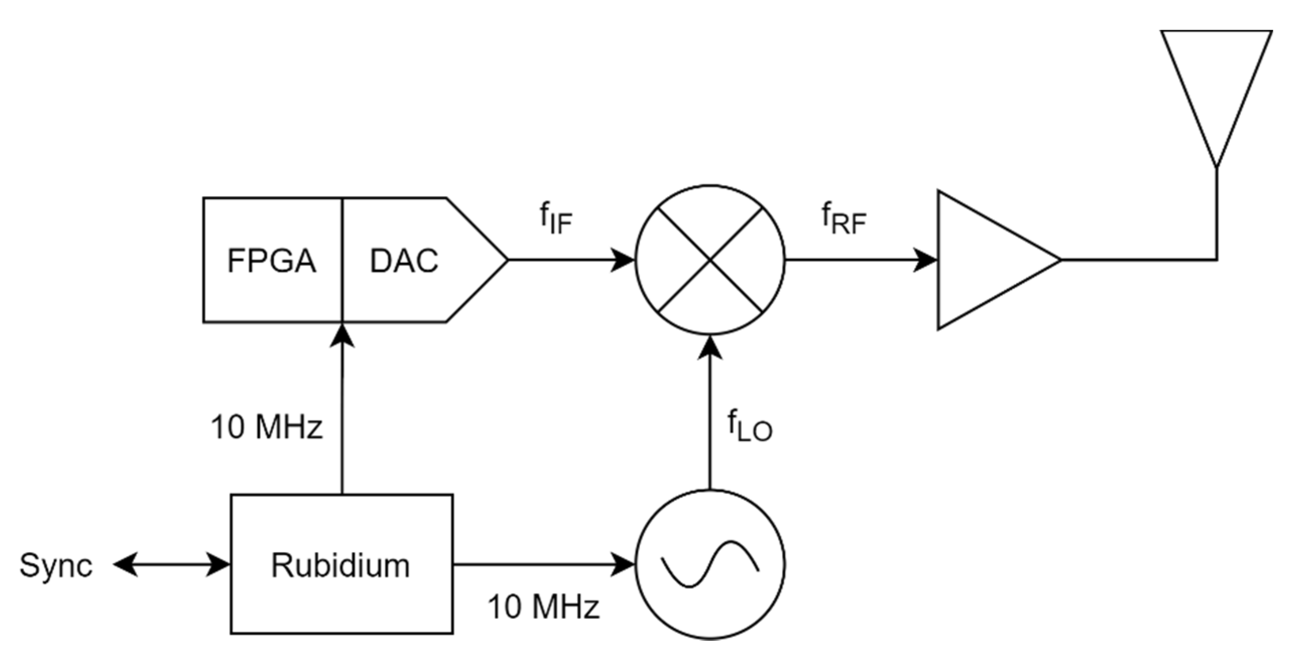
The block diagram of the transmitter is shown in Figure 3, with the hardware components referenced in Table 1. The core of this part is composed by the VC707 evaluation board manufactured by Xilinx. This hosts a Virtex-7 FPGA and acts as the sequence generator. The sounding signal generated within the FPGA is sent to the digital-to-analog converter (DAC), an AD9161. The converter has been configured to produce a signal centered in 4 GHz, which is then mixed and upconverted to 28.65 GHz. The mixer is the double balanced M1826W1 from MITEQ. The local oscillator (LO) port of the mixer is connected to the signal generator HP 83650B. All of the clocks in the components are locked to a rubidium reference of the model PRS10, manufactured by Stanford Research Systems. The signal is amplified before transmission; the model of the amplifier is ERZ-HPA-2700-4200-27 from ERZIA. Two linearly polarized antennas from Flann Microwave were used in the different tests: an omnidirectional antenna and a standard gain horn.
Several different pseudorandom binary sequences (PRBS) are stored within the FPGA. This allows to switch to the one that best fits each scenario without even reprogramming the device. The chip rate with which the sequence is generated depends on the clock provided to the transmitter. For the current campaigns, the DAC provides a 125 MHz clock to the FPGA. Linear feedback shift registers that produce 4 chips per clock cycle in parallel allowed to generate PRBSs with a chip rate of 500 Mcps. This translates into an RF null-to-null bandwidth of 1 GHz.
2.2. Receiver
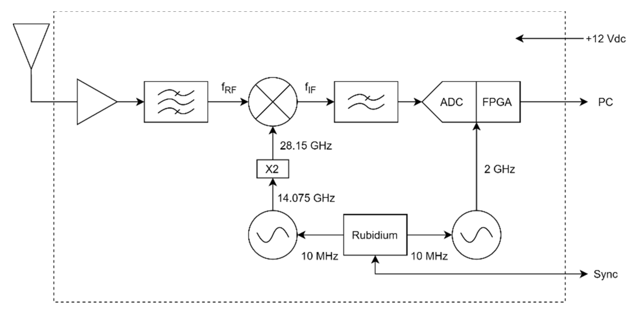
Figure 4 shows the block diagram of the receiver, with its components referenced to Table 2. The omnidirectional antenna, from the same model as the one shown in the transmitter, has a support that eases installation on the roof of a car. Its low directivity matches the typical scenario for the mobile end of a radio link. The signal is then filtered, amplified, and down-converted to intermediate frequency (IF). The IF signal, centered on 500 MHz, is passed through a low-pass filter (LPF) and is then sampled by the analog-to-digital converter (ADC). The samples are processed by another Virtex-7 FPGA. As in the transmitter, all clocks are locked to a 10 MHz rubidium reference.
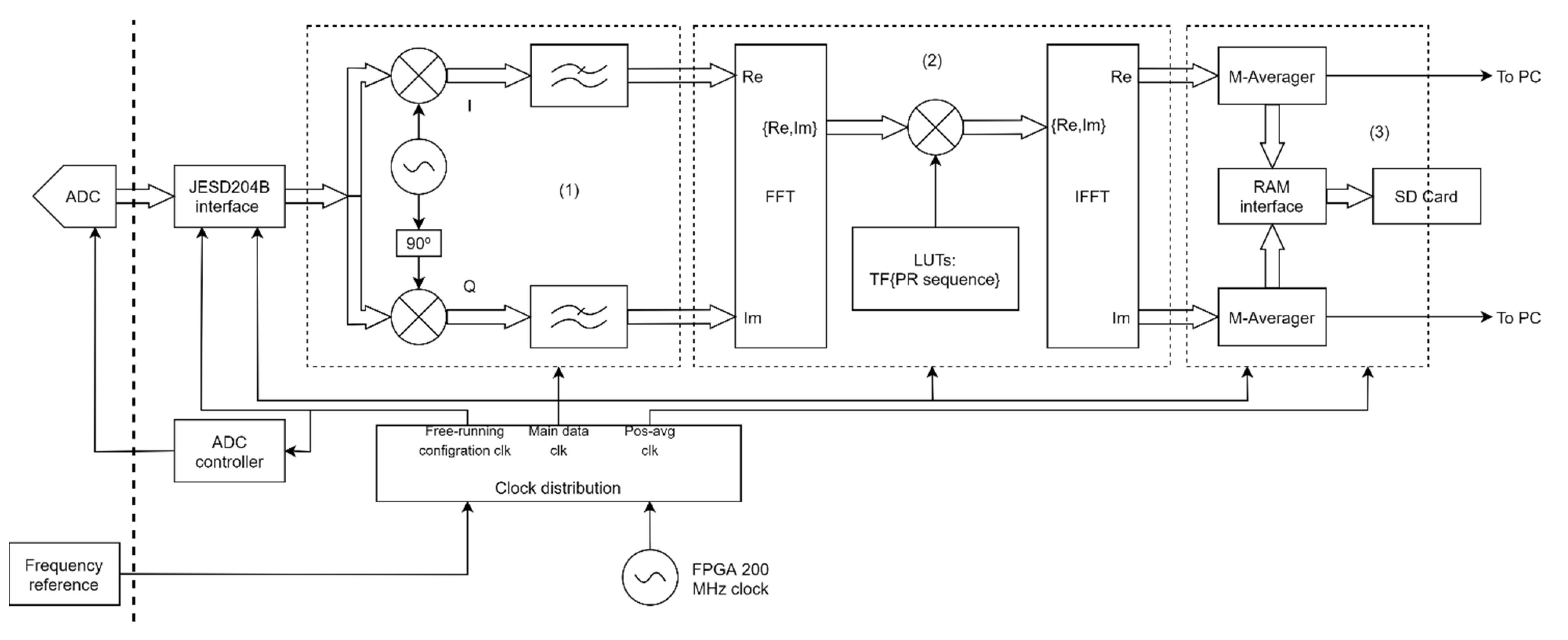
A scheme of the FPGA operation of the receiver is provided in Figure 5. In this image, thick arrows represent the flow of the received data, meanwhile the thin ones are assigned to clock and control signals. After sampling, the received signal is passed through a quadrature demodulator, marked with (1) in the image. Baseband I and Q components are then converted to frequency domain and multiplied by the frequency response of the transmitted sequence. This stage is labeled as (2) in Figure 5. Conversion to time domain after this allows to obtain the impulse responses of the channel. Finally, time-domain averaging of successive measures is implemented in order to improve dynamic range and to reduce data volume, which eases data handling. This corresponds with the label (3) in the scheme. A more detailed insight into the receiver is given below.
First of all, a JESD204B module interfaces the data signals between ADC and FPGA. JESD204B is a protocol intended for achieving high data rates between logical devices and converters, so a number of these implement this interface. The signal coming from the data interface is input into the quadrature demodulator. As the sampling frequency, fs, is equal to 2 GHz and the intermediate frequency is fIF = 500 MHz, the sinusoids required to demodulate the signal to baseband have an integer number of samples per cycle. Thereby, by multiplying the input signal by the sets {0, 1, 0, −1} and {1, 0, −1, 0}, the baseband branches I and Q are obtained. This allows to simplify the quadrature demodulator. Both branches are then filtered to keep only the baseband component.
The following stage is the correlator. To compute the correlation between two signals, the dot product of one by the other has to be evaluated in all possible delays. One way of achieving this is by using a matched filter [26]. Nevertheless, although it is an optimal way of performing the correlation, it presents some practical issues. The order of the filter is equal to the length of the sounding sequence, so, in a real-time application with long sequences, it is impractical to implement such a long filter.
It is well known that the convolution of two signals in the time domain is equivalent to their product in the frequency domain. As the operation of any filter is basically a convolution, it is possible to substitute the digital matched filter by a multiplication in the frequency domain. The Fourier transform is efficiently implemented in hardware through the fast Fourier transform (FFT) method. This allows to circumvent the need of using a matched filter of great order.
After the FFT block, the signal is multiplied by the frequency response of the transmitted sequence. As the latter is stored in lookup tables (LUTs), it can be computed beforehand. Moreover, several sequences can be used without changing the design: it is straightforward to switch between LUTs using the switches of the evaluation board. Of course, the length of the FFT has to be at least larger than that of the sequence, which leads us to the following point.
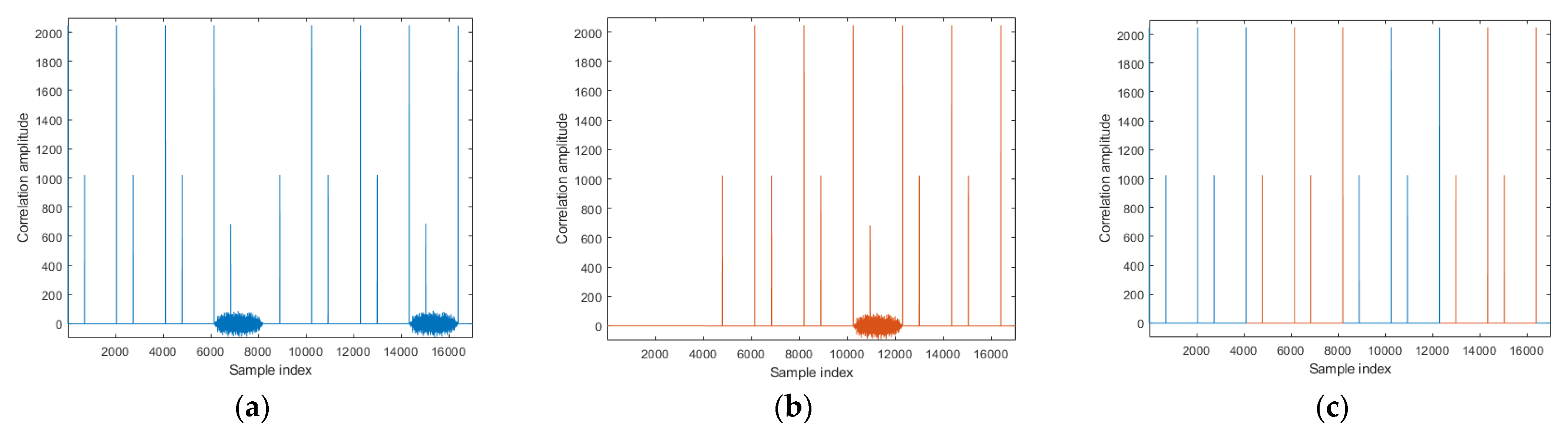
FFT is a discrete operation that works by performing a transform on a block of samples at its input. After one block is transformed, the next one is processed and so on. Thanks to pipelining, it is possible for the FFT to operate continuously: it can start picking the first sample of the next block just after it has taken the last sample of the current one; independently of the latency, it outputs the results. However, dividing the received signal in blocks may affect the channel estimation. This happens if the PRBS received through a propagation path is split between two different FFT blocks. In this case, part of the energy corresponding to a propagation path (which spans a complete duration of the PRBS) is taken in one FFT cycle and the rest in the next one. This results in an erroneous channel estimation. To overcome this problem, the received signal is processed in parallel by two correlator modules, one of them operating with a delay of half an FFT block with respect to the other. The outputs of both correlator modules are then combined in such a way that a perfectly continuous channel response is obtained. Figure 6 is used to illustrate this. In this example, simulated with the software Matlab, a periodical PRBS-11 is passed through a simple two-tap channel (h(n) = δ(n) + 0.5·δ(n − 700)) and correlated in the frequency domain using a FFT length of 8192 samples. Echoed sequences whose first chip falls within the last 2046 samples of the transform produce distorted results. This can be seen as a noisy region in the last 2046 samples of each block. In the delayed FFT, the samples located in the first half of a block correspond in time with those of the second half of the non-delayed FFT. Therefore, to obtain a continuous signal equivalent to the theoretical correlation, the first half of the block of the delayed module’s output is appended after the first half of the original module and so on. The second halves of each block, with the distorted samples, are discarded. This method is equivalent to the time-domain correlation if and only if the length of the FFT is at least twice the length of the sequence.
Both real and imaginary parts of the output of the correlator are finally averaged before storage. The main reason to perform this operation before storing the samples is to reduce both the noise and the data volume to be stored. This will also reduce the data rate the FPGA has to handle to an external storage device. The reduction of data will allow longer periods of continuous channel sounding, considering that the available memory is limited. Nevertheless, increasing the size of the averaging reduces the sampling frequency at which the sounder probes the channel. This poses a tradeoff between the maximum continuous measurement time on one hand and the maximum measurable Doppler frequency on the other. The reduction of the latter limits the speed at which the sounder can be moved. It should be noted, however, that increasing the averaging also improves the dynamic range of the sounder.
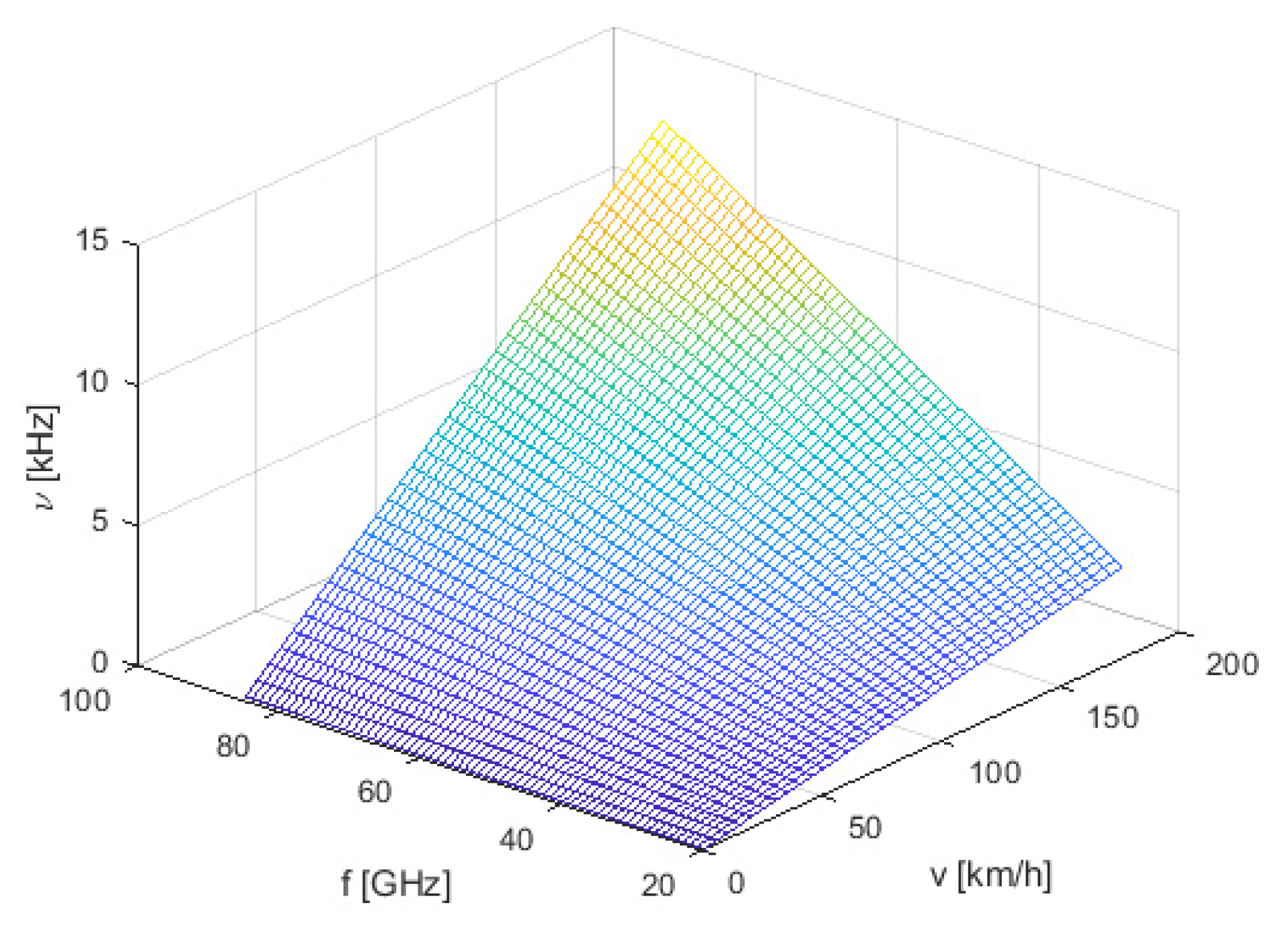
In Figure 7, a reference for Doppler effects at different carrier frequencies and speeds is given. It corresponds to the maximum Doppler shift, i.e., the absolute shift when the angle of the incident wave and sounder velocity are parallel (0° or 180°). This has to be considered when using the sounder at different frequencies for high-speed channels. Higher speeds generate higher Doppler shifts. The same is true when increasing the frequency. As the maximum Doppler is fixed (for a given averaging size), higher frequencies will impose more restrictive limits on the maximum speed at which the sounder can move. In the current scenarios, at 28.65 GHz, the maximum speed is 287.74 km/h for an averaging size of 16 responses, i.e., a maximum allowed shift of 7.63 kHz. The limitation on speed imposed by the maximum Doppler has to be respected: the angle of the line-of-sight (LoS) path between transmitter and receiver can be controlled in a measurement session, but the echoes can come in any direction.
Finally, the data are exported. As the data rate is quite large even after averaging, the samples are initially written in real time to the synchronous dynamic random-access memory (SDRAM) included in the VC707. After this intermediate step, which defines the duration of a single continuous channel measurement, the data are exported to an external storage. We have chosen secure digital (SD) cards for the sake of simplicity, but faster setups might be possible in other designs, e.g., using the peripheral component interconnect express (PCIe) interface of the board. Exported data consists of the M-averaged real and imaginary parts of the estimated channel impulse response. These may then be processed on a computer to represent the power-delay profile (PDP), Doppler spectrum, channel correlation functions, etc. No computer is required during the measurement campaign itself, but one can be optionally connected to the FPGA to obtain a brief glimpse into what is being received, as shown in Figure 5. By quickly processing a small number of responses at the output of the averaging blocks, it is possible to verify that the setup is currently working and the full measurement process can begin.
2.3. Sounder Configuration and Parameters
In Table 3, the current sounder parameters are shown. Notice that some of these are easily tunable according to the specific needs of the channel characterization campaign. The total cost of the core of the system (without RF frontend) is below 12,000 €. The RF frontend may suppose variable costs.
These performance values are achieved when a PRBS-11 is used. The sounder configuration may be changed by swapping the sounding sequence. It is possible to switch to less-order sequences to increase the channel sampling rate, the amount of channel samples per full operation interval (the length of time in which a continuous acquisition can take place), and the maximum Doppler shift (and hence the sounder displacement speed). This comes at the cost of dynamic range and maximum unambiguous delay.
Another important aspect of the design is that the length of a single continuous measurement is limited by the size of the SDRAM aboard the VC707. Currently, this is a 1 GB card. Higher capacity memories would increase the aforementioned operation interval. For example, a 4 GB card would increase the uninterrupted measurement time to 17.18 s. It is also possible to average more channel responses to increase the operation interval. The previously mentioned parameters are obtained with an averaging size of 16 responses.
Due to the larger capacity of SD cards, measurements resulting from several operation intervals may be recorded in a single SD card.
Last but not least, frequency synchronization plays an important role in the operation of the sounder. Excessive phase noise or a frequency offset between transmitter and receiver may degrade the retrieved results. As such, highly stable synchronized frequency references have to be used in both ends. Typically, in the literature, cesium or rubidium clocks have been mentioned for this purpose. Cesium standards offer better performance, but their higher bulkiness and cost made rubidium clocks the prominent choice [27]. As stated in the previous subsections, we have used two rubidium frequency standards of the model PRS10 from SRS to supply all frequency sources in each side of the sounder with a common reference. This way, we can ensure that all frequencies used within the transmitter and the receiver are locked to a stable reference. This excludes the clocks used within both FPGAs to program the converters, as they do not influence signal paths in any way. In the receiver, the internal clock of the FPGA is also used in the averaging and storage modules. A first-in-first-out (FIFO) queue interfaces both clock domains so that the samples are not affected.
Nevertheless, as transmitter and receiver are not physically linked during the measurements, both frequency references have to be synchronized. A 1 pulse-per-second (1PPS) port is usually given in high-precision frequency sources. The procedure consists in the transmission of a narrow pulse with a pulse-repetition frequency (PRF) of 1 Hz. Of course, the long-term stability (i.e. the proximity of the PRF to 1 Hz after hours of operation) of the PRF source is paramount. The short-term performance (i.e. the jitter between successive rising/falling edges of the pulse) is also important, but the PRS10 provides an exponential running-average process that allows to reduce its impact with the tradeoff of larger locking times.
Global positioning system (GPS) modules may provide 1PPS outputs, which have very good long-term stability due to the use of GPS signals. The aforementioned averaging process is critical in this case, as the short-term jitter in the GPS 1PPS can reach between 50 ns to 300 ns. Alternatively, the 1PPS output of one PRS10 can also be used to train the other, having the advantage of a lesser jitter, which allows a faster lock without the averager. This second option was used in all measurements. This way, there is no concern about bad GPS signal coverage in the locking process. Three hours are enough to achieve a proper synchronization, as per manufacturing specifications. The equipment is kept inside the laboratory, connected to the electrical grid, so that the batteries are not discharged.
When the 1PPS ports are disconnected, the clocks start to slowly lose synchronization. Before this disconnection, less than 1 ns (half the delay resolution) drift between the two clocks is observed in a 24 hours’ period. As so, at this instant, the frequency offset between both units is negligible. Laboratory tests have shown that a drift of less than 10 ns happens within the first hour after disconnection for different ambience temperatures. No more than 30 ns of drift have been found in the first 4 h. As our continuous acquisition times are in the order of several seconds and we do not measure absolute delay, this stability is enough for our purposes.
2.4. Campaign Settings
To test the sounder as well as to obtain real channel measures on the 28 GHz band, different campaigns were scheduled. The first of them served to test the sounder statically inside the laboratory. In the second campaign, the receiver was mounted in a car, which proceeded to move past the transmitter at slow speeds (around 25 km/h). Finally, in the third campaign, the transmitter was placed on an elevated pass above a highway. In this one, measurements were conducted at high speeds (around 120 km/h).
As shown in Table 1, two different antennas were attached to the transmitter depending on the campaign. The omnidirectional antenna was used both inside the laboratory and on the low-speed campaign. The directional antenna, with a 20 dBi gain, was used in the highway measurements.
Before the start of every campaign, the 1 pulse-per-second (1PPS) ports of both rubidium clocks were linked together so that synchronization was achieved, as stated before.
2.4.1. Laboratory Setup
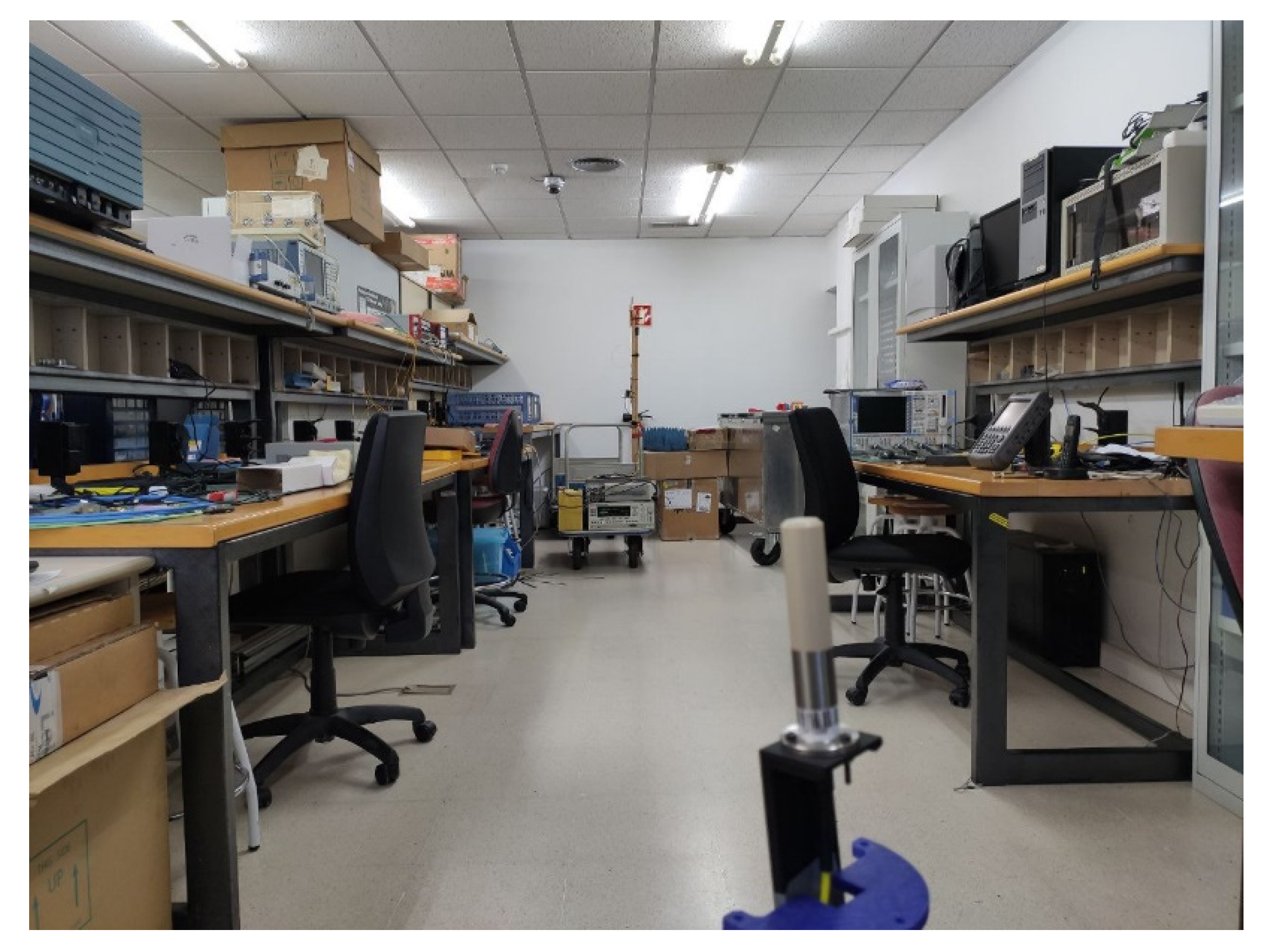
In this scenario, basic functionality of the sounder was tested. No relative movement between transmitter and receiver happened during these tests. In Figure 8, a full picture can be seen.
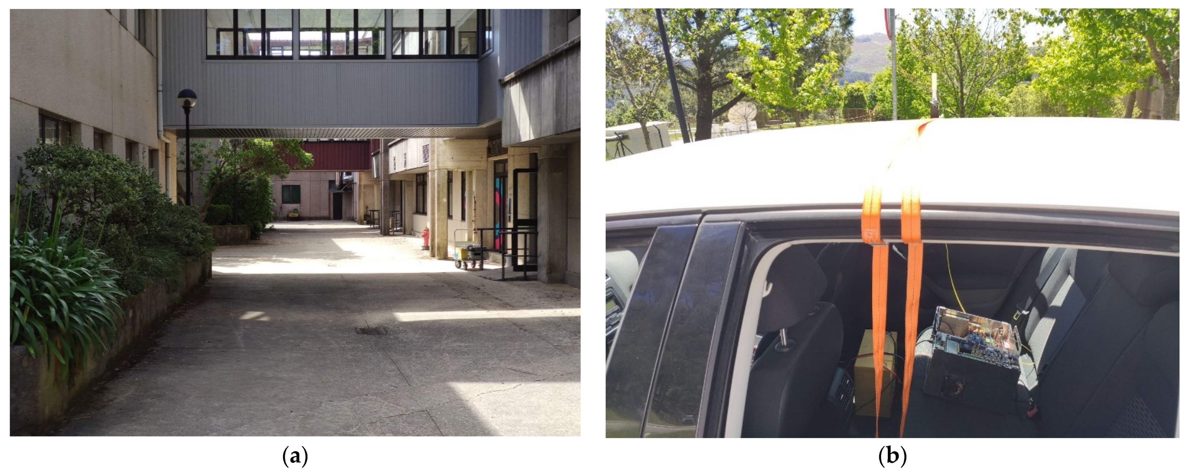
2.4.2. Low-Speed Setup
2.4.3. Highway Setup
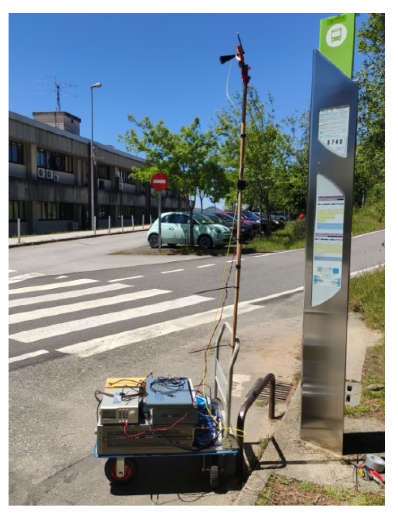
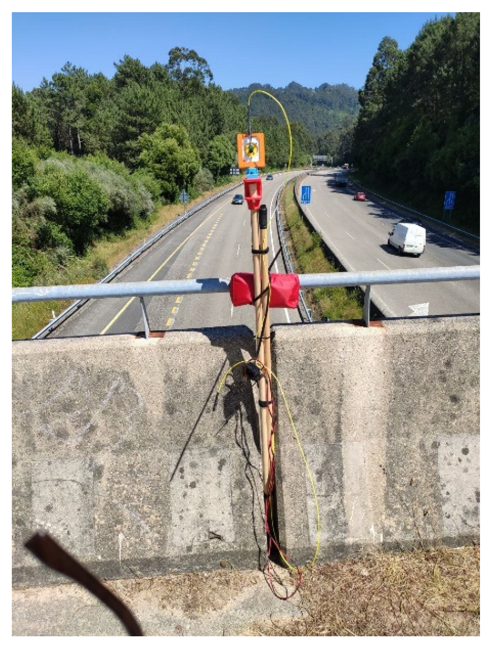
To achieve the highest Doppler shifts that a mobile communications channel can present, high speeds have to be reached during the measurement. For this purpose, a suitable portion of a highway had to be selected. For the sake of simplicity, the transmitter was chosen to be placed on an elevated pass, with the car carrying the receiver passing below. A picture of the transmitter can be seen in Figure 10. The chosen location allowed the vehicle to reach maximum legal speed (120 km/h) by the time the elevated pass was overtaken.
3. Results
3.1. Laboratory Tests
As it was previously explained, the first set of tests was conducted inside the laboratory so that basic operation of the sounder could be ensured. In Figure 11, the PDPs computed after a single continuous run of the acquisition process are represented. Besides the 16-average applied within the sounder, a further average of 256 responses was computed for ease of representation. For all subsequent calculations, a threshold was applied over the received data so that the residual noise does not affect the results. This threshold was applied in both the real and imaginary sets in such a way that every sample which did not surpass at least one of the thresholds was discarded. Samples not discarded were fully considered, even if one of the two values did not reach the threshold. As can be seen, there are different multipath contributions with fixed delays. The full average of the measurement is shown in Figure 12, which corresponds to a typical PDP of a LoS channel. Note that we have not calibrated sounder’s response. As a consequence, some distortion, in the form of peaks with delays lower than the direct contribution, was introduced. Due to the frequency-domain approach, this distortion could be easily removed, as stated in [27]; it was not done in this work, however.
An interesting parameter of wideband channels is the delay spread, which is the well-known square root of the second central moment of the PDP. In essence, this parameter quantifies how the energy transmitted at a single time instant in the transmitter is scattered before arriving at the receiver: it is the standard deviation of the delay of multipath components weighted by their respective energy, as shown in Equation (1):
where is the mean delay, computed according to Equation (2):
For this channel, the value of is 10.67 ns, which agrees with the dimensions of the environment.
3.2. Low-Speed Scenario
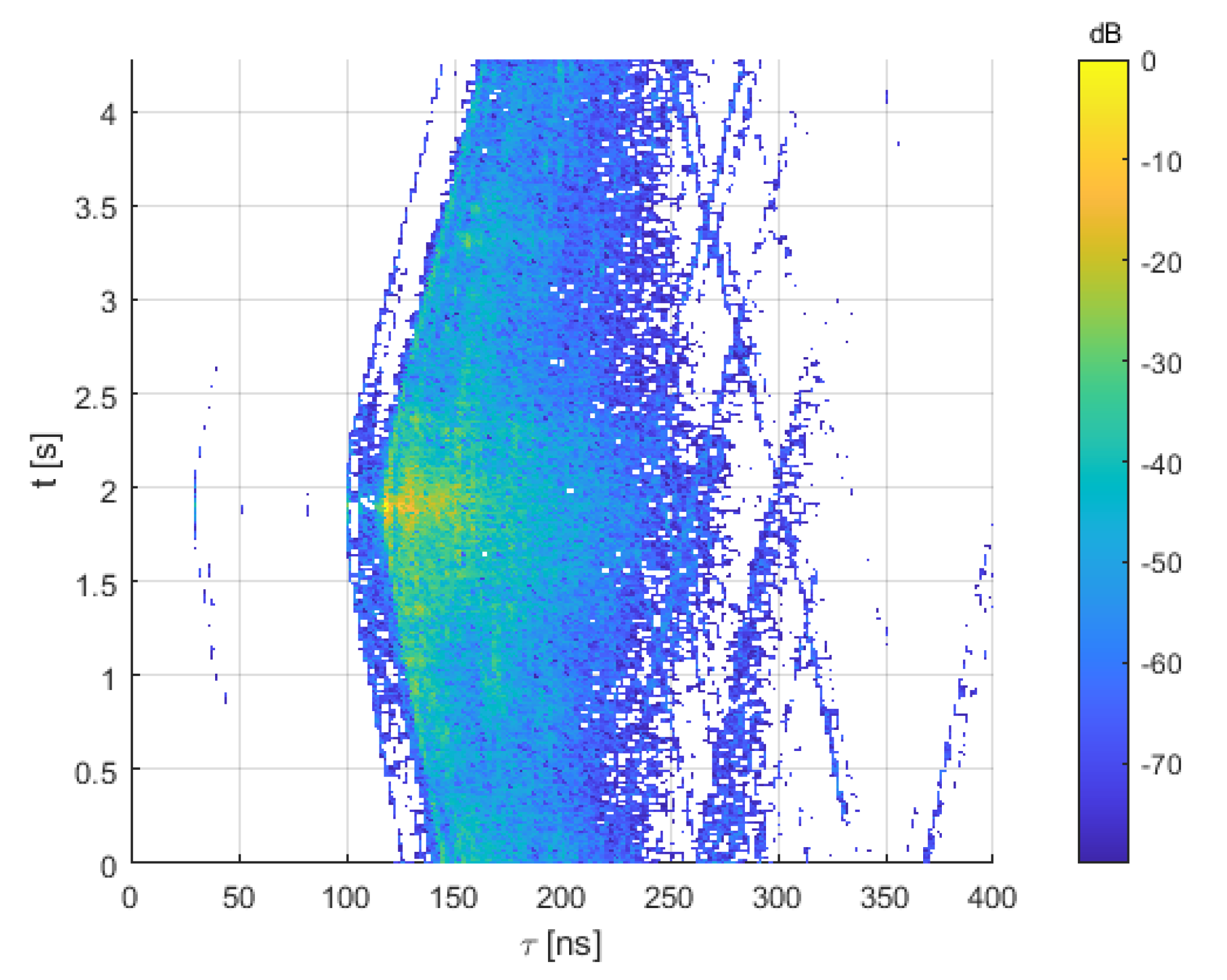
The measured data for the alley are depicted in Figure 13. It can be seen that the positions of the different contributions vary with time in contrast with the former scenario. This is due to the motion of the receiver along the scenario. During the first 2 s of the measure, the car is approaching to the transmitter. This corresponds to the main contribution, i.e., the direct path, arriving earlier. After the transmitter is surpassed at around 2 s, the direct path gets more delayed with time.
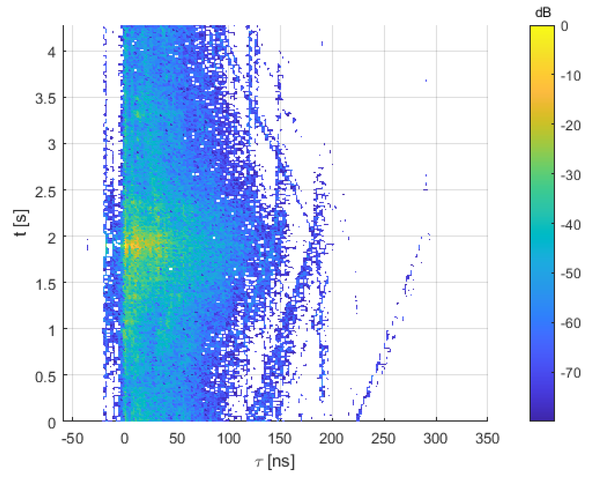
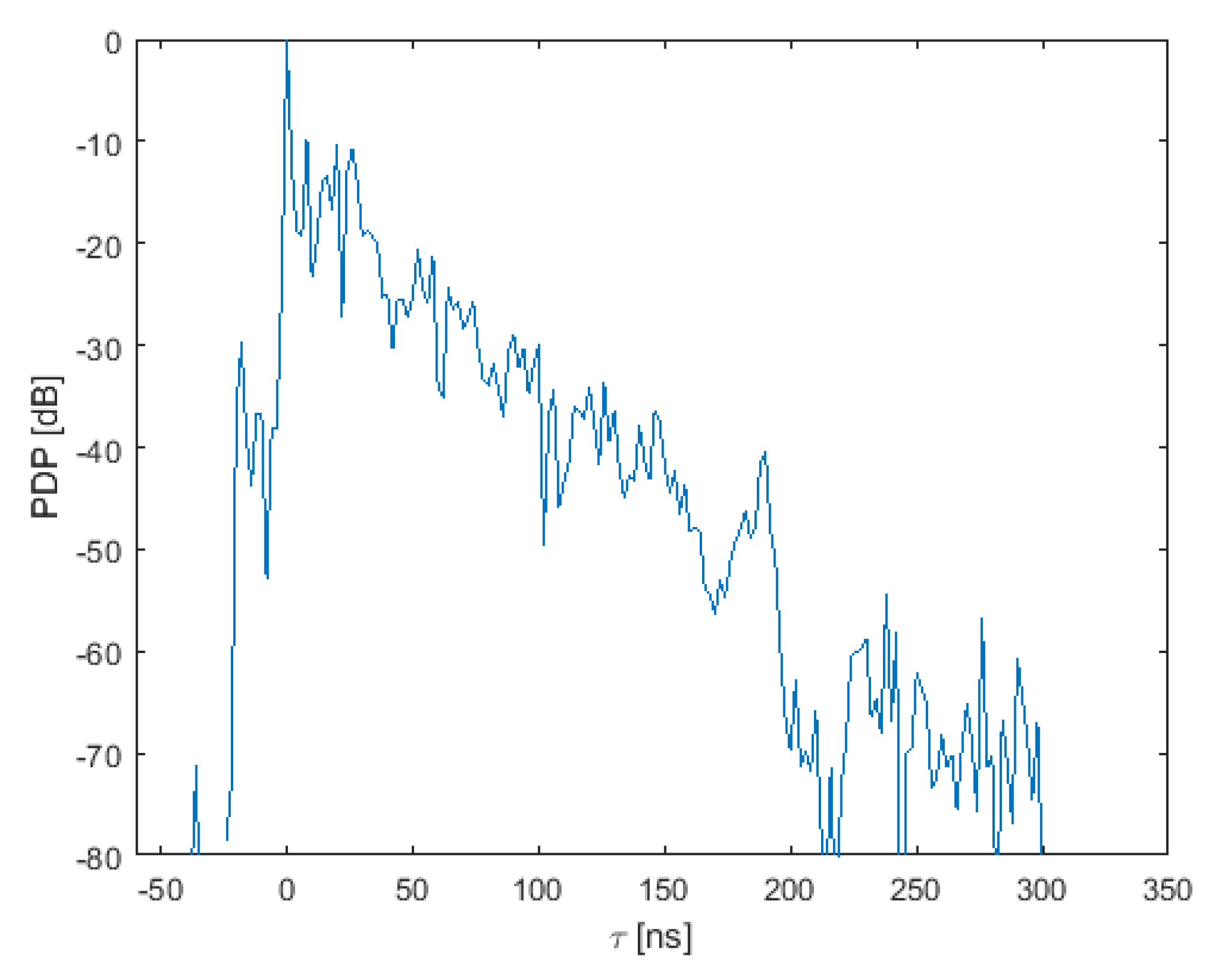
To obtain the Doppler spectrum of a single component, the channel responses were aligned in delay before computing the Fourier transform. This was also necessary to averaged PDPs. To perform this alignment, the main path, having the highest power, was chosen as the reference. The result is depicted in Figure 14. With this, it is possible to compute a fully averaged PDP, which is shown in Figure 15. If we used this PDP to obtain the delay spread, we would obtain 15.79 ns, which is reasonable for this scenario.
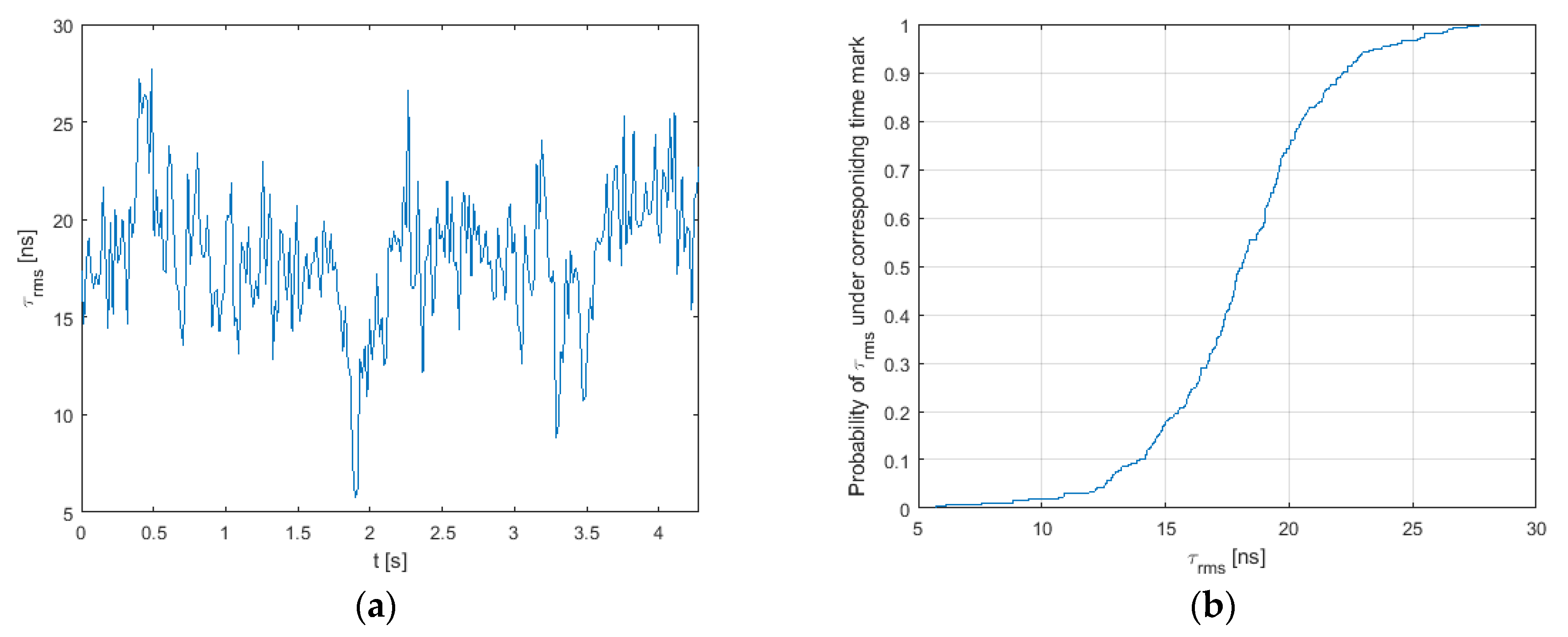
Nonetheless, from the previous plots, we can see that the channel varies within the 4.29 s of continuous channel sounding. This is a common characteristic of non-stationary channels. It is possible to observe the variation of the channel characteristics, as the delay spread throughout the measurement process. To achieve this, the delay spreads corresponding to groups of 256 consecutive channel responses were calculated and are shown in Figure 16a. The delay spread varies from 5.7 ns to 27.7 ns. The cumulative distribution function (CDF) can be used to obtain the statistics of this parameter, as depicted in Figure 16b. From it, we can obtain that the 99% of the time the delay spread is below 26.62 ns.
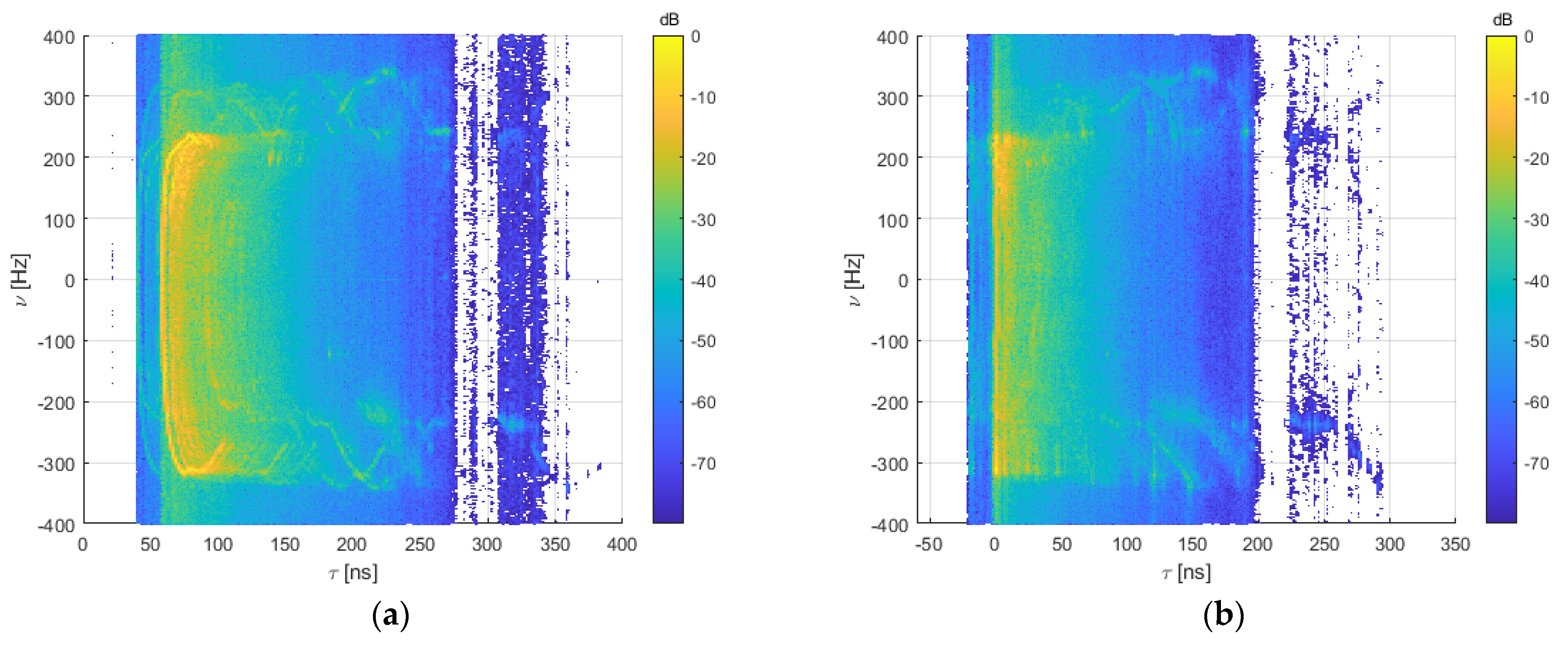
It is also of interest to obtain the delay-Doppler spectrum (scattering function) of the channel. This is computed as the Fourier transform of the samples corresponding to the different delays. In Figure 17, the delay-Doppler spectra of this campaign, computed both from the original and the aligned responses, are depicted. The asymmetry between positive and negative frequency shifts comes from the fact that, in the initial seconds of the data acquisition, the car is still accelerating to the maximum speed that it can safely reach in the scenario. Therefore, positive frequencies (receiver closing distance to the transmitter) reach lesser values. A close-up of to the Doppler spectrum of the main component can be seen in Figure 18.
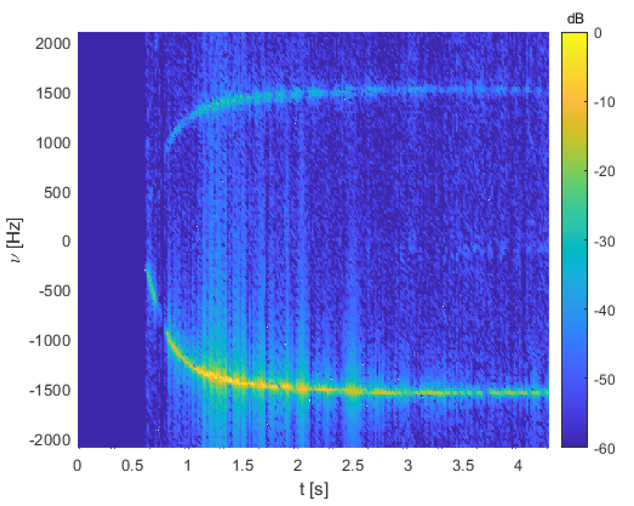
Nevertheless, as the channel is non-stationary, and the sounder is able to probe it very fast, it may be of interest to not only watch the Doppler spectrum of the full measurement but also its evolution with time. Thereby, we divided the set of responses into chunks of equal length to compute the Doppler spectrum of individual delays. This had an impact on the frequency resolution of the resulting spectrum, as fewer samples were available per FFT. We chose an FFT size of 256, resulting in a step of 29.82 Hz. The time-domain resolution with which we calculated this spectrum was, hence, 16.78 ms. Decreasing the FFT size would result in more time axis samples at the penalty of worsening the frequency-domain resolution. In Figure 19, the evolution with measurement time of the Doppler frequency associated to the main delay path is shown.
The transition from positive to negative shifts corresponds to a radial change of direction with respect to the reference point defined by the transmitting antenna. As this one is static, and the car is moving in a straight line, this variation highlights the instant when the car surpasses the transmitter. To verify the proper operation of the sounder in the Doppler domain, a GPS system was used to record the speed of the receiver. In Table 4, the comparison between expected Doppler shift and its measured value is presented. To retrieve the measured values, the FFT size was doubled in order to improve frequency resolution with respect to Figure 19. This corresponds to a frequency resolution of 14.91 Hz and a time resolution of 33.55 ms. In the table, v represents vehicle speed, α is the angle between vehicle velocity and the incident wave from the direct propagation path (i.e., a straight line between the car and the transmitting antenna), and νth and νmeas are the expected and measured shift, respectively.
As the resolution is 14.91 Hz, there is an error margin of ±7.45 Hz from the measured value. It can be seen that the expected shift always falls within this range.
3.3. Highway Scenario
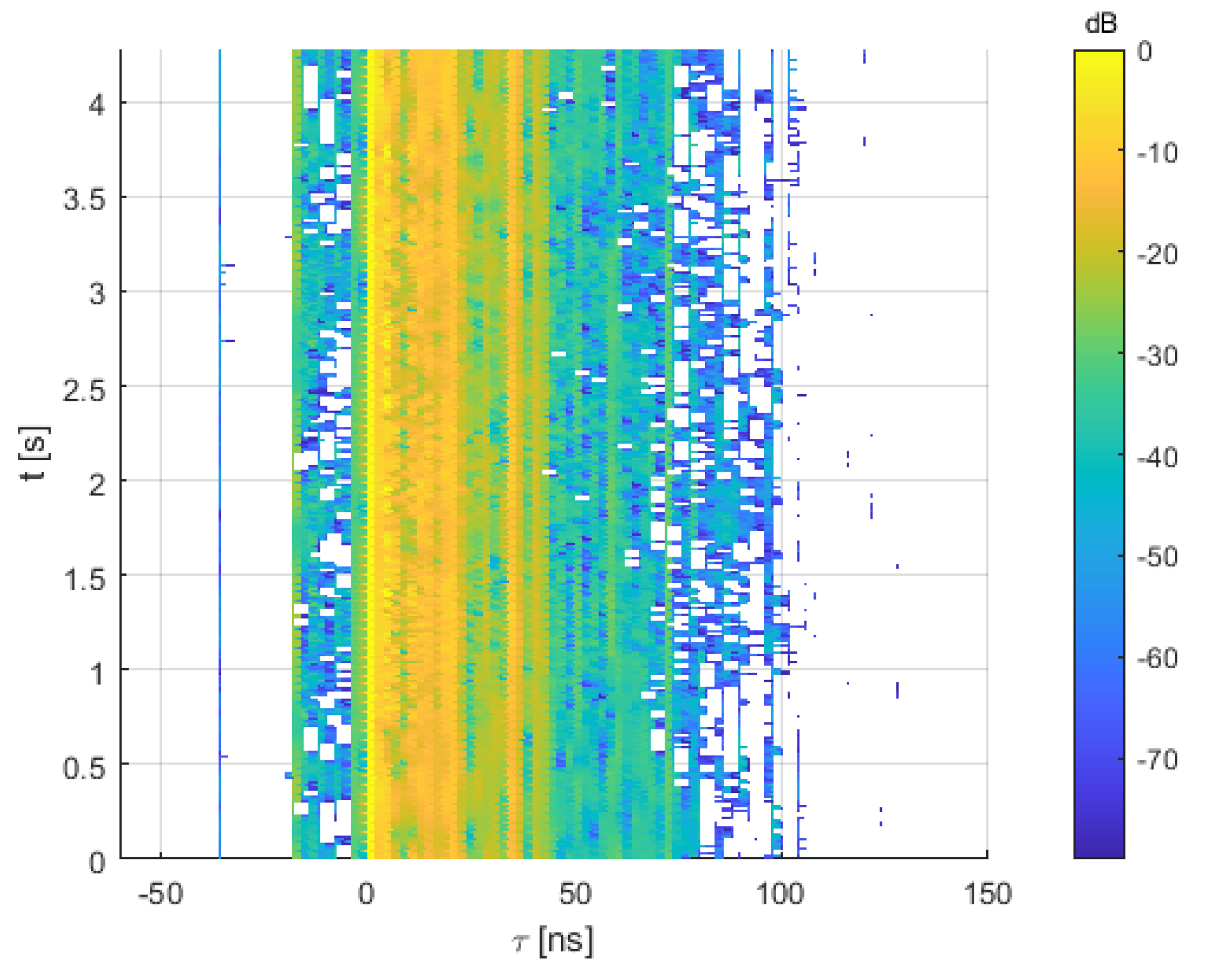
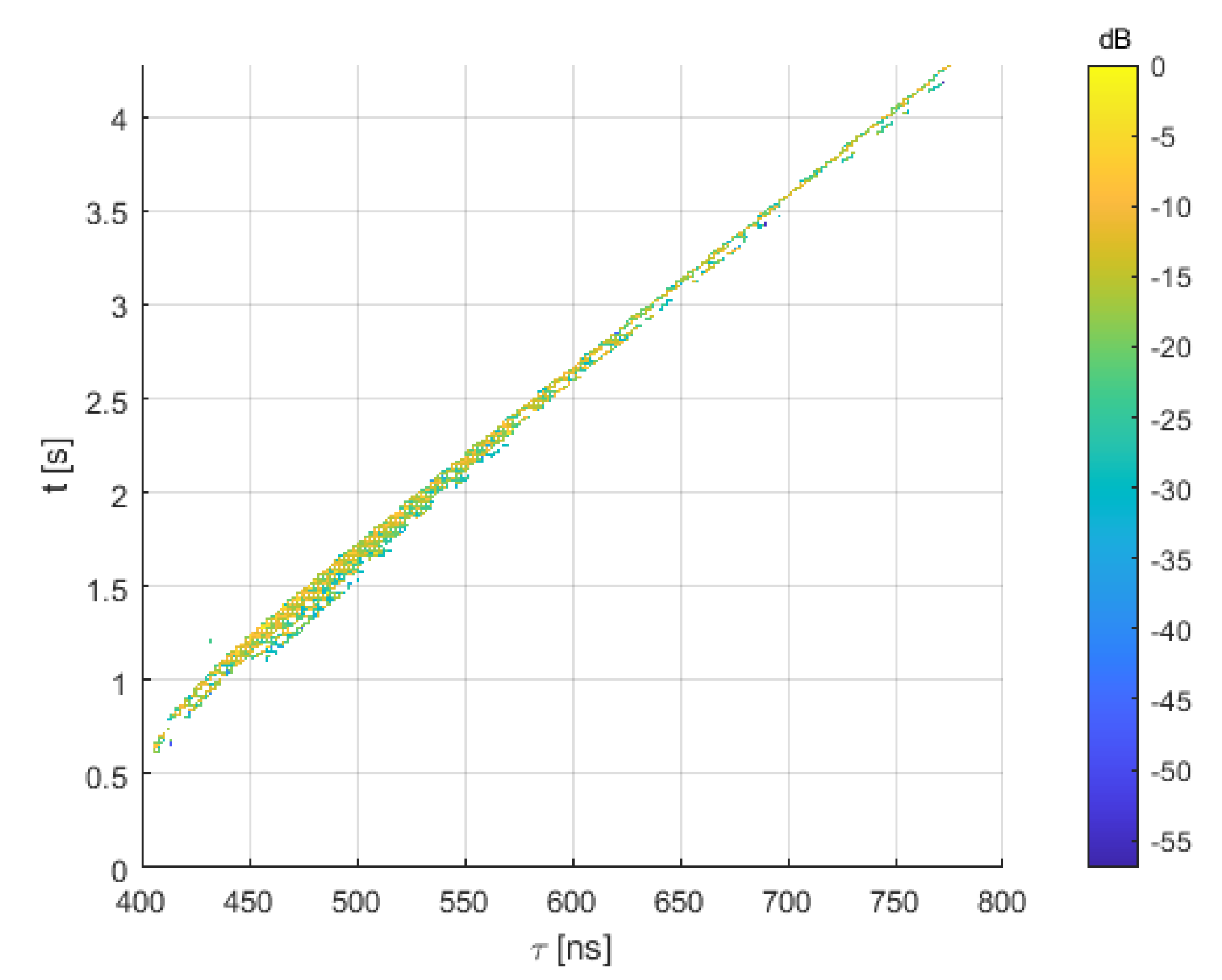
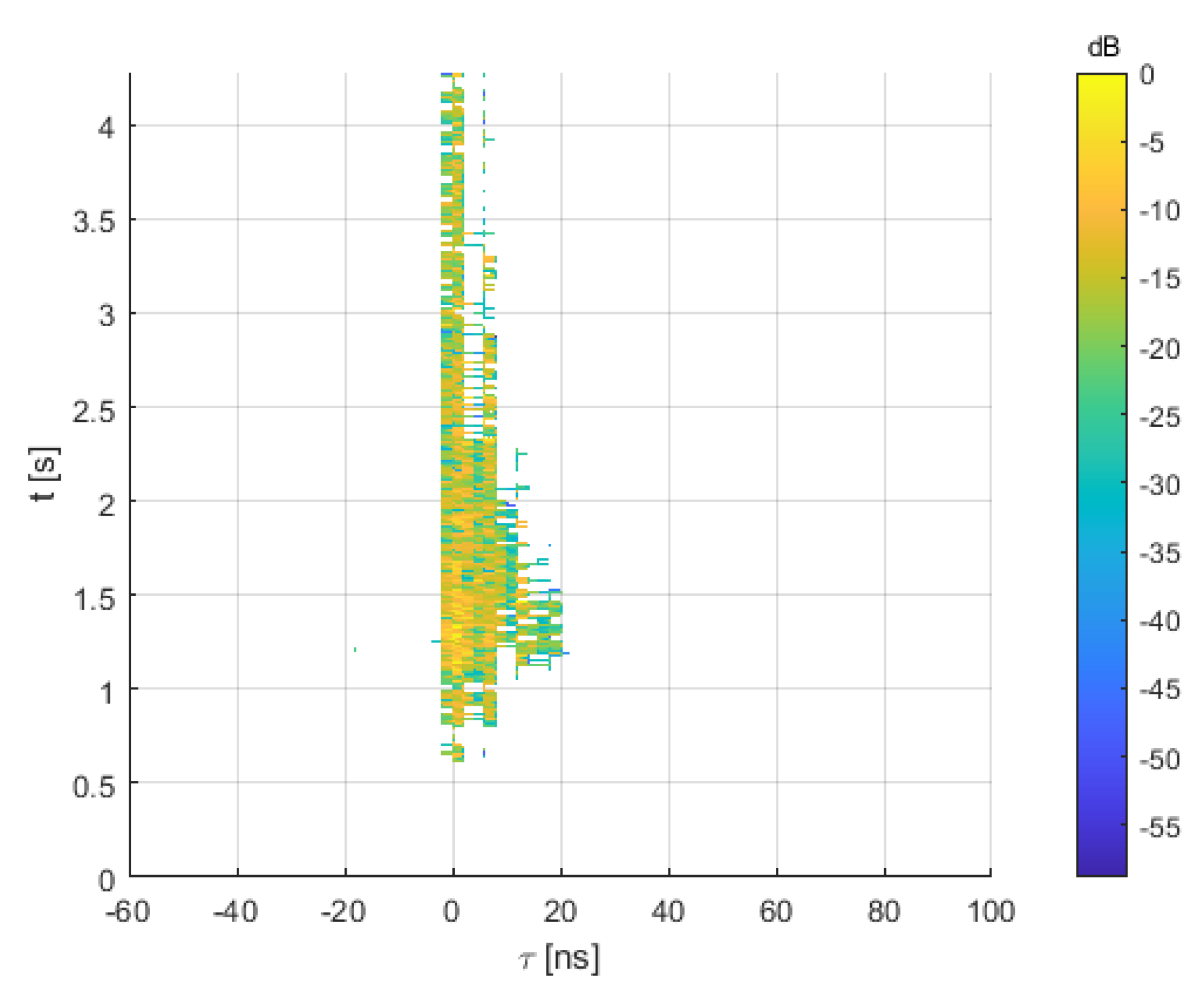
In Figure 20, the PDP is represented. At first glance, there are various significant differences from Figure 13. First of all, the variation of the response with the time is significantly quicker due to the higher velocity. In the former scenario, we were accelerating from the starting point towards the transmitter and passing by its side with a maximum speed of no more than 25 km/h. In this one, we started to capture after passing under the transmitter in the highway, having already reached a speed close to 120 km/h. As we were moving away from the transmitter this time, the position of the main component was only delayed with each measure, in contrast with Figure 13. Another thing to note is the fact that less multipath components seem to be present. This was expected, as a highway has commonly a significantly lesser number of scatterers and placed farther away. This last aspect, together with the free space attenuation at 28.65 GHz, makes the echoes arrive with large attenuations due to the long paths.
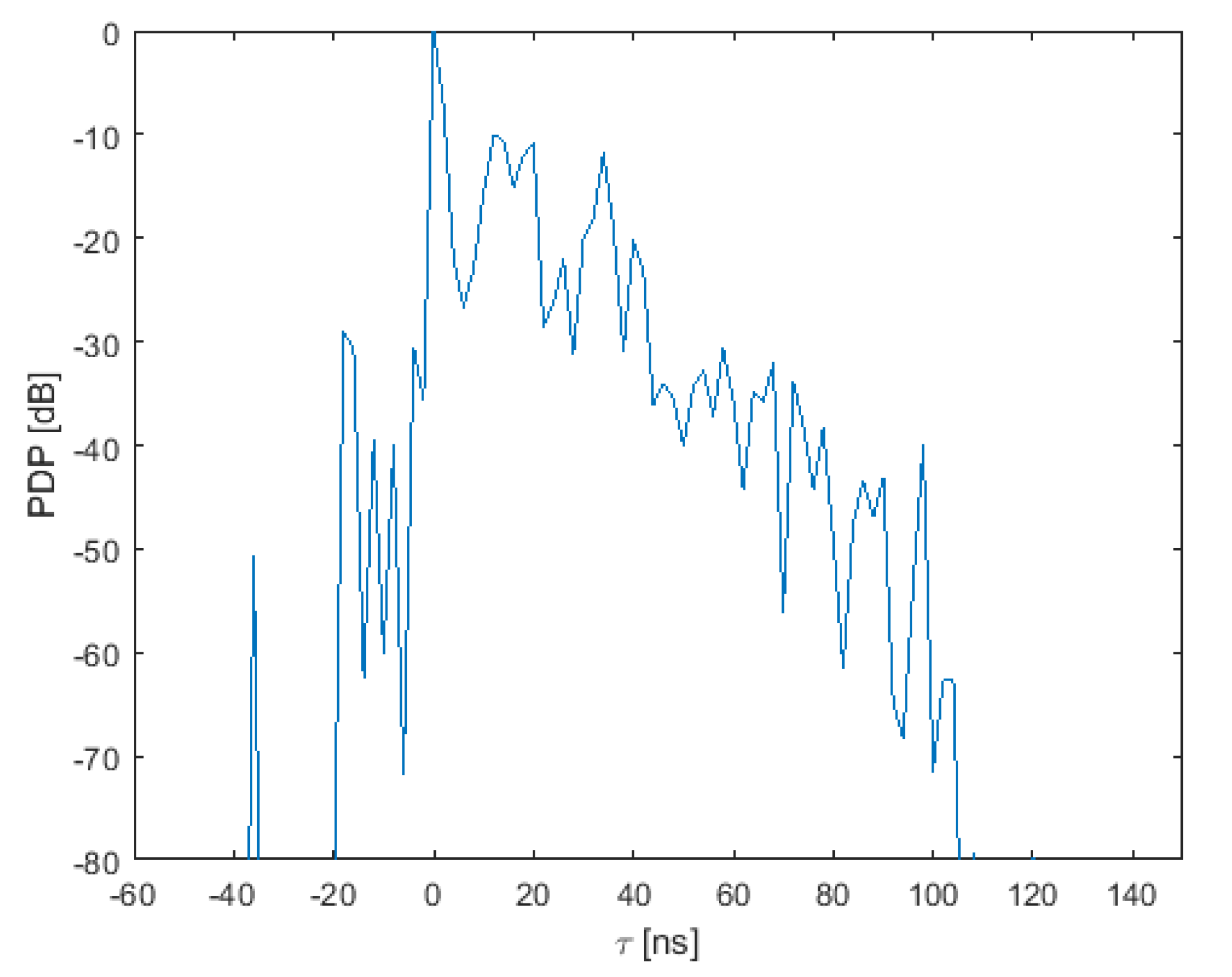
By aligning with respect to the main component, the PDPs of Figure 21 were obtained. The fading of the echoes with respect to previous campaigns becomes more clearly visible now. It is important to note the null values during the first 0.75 s. These correspond to the car still located below the bridge and out of the main lobe of the transmitting antenna. For the following calculations, these samples have been removed.
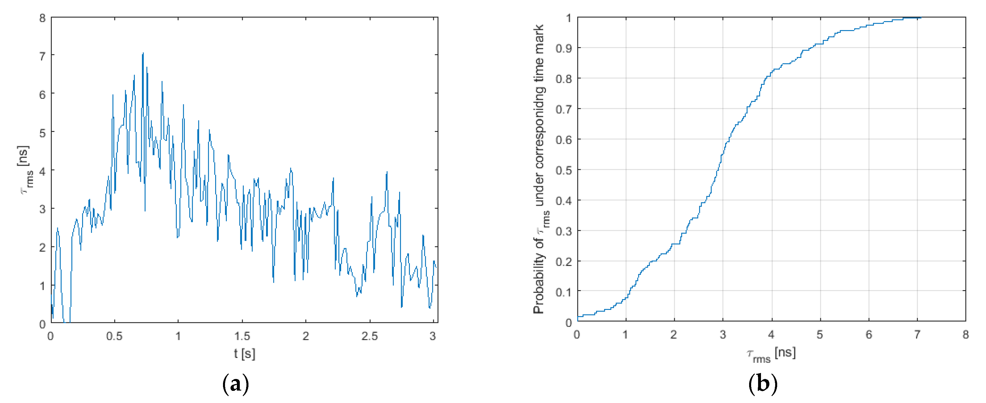
Analogously to the former case, it is possible to compute the RMS delay of the channel. The results are shown in Figure 22. As it was anticipated, due to the lesser amount of echoes, the values of the delay spread are remarkably lower to those of the alley. A value of 6.63 ns is not exceeded the 99% of the time.
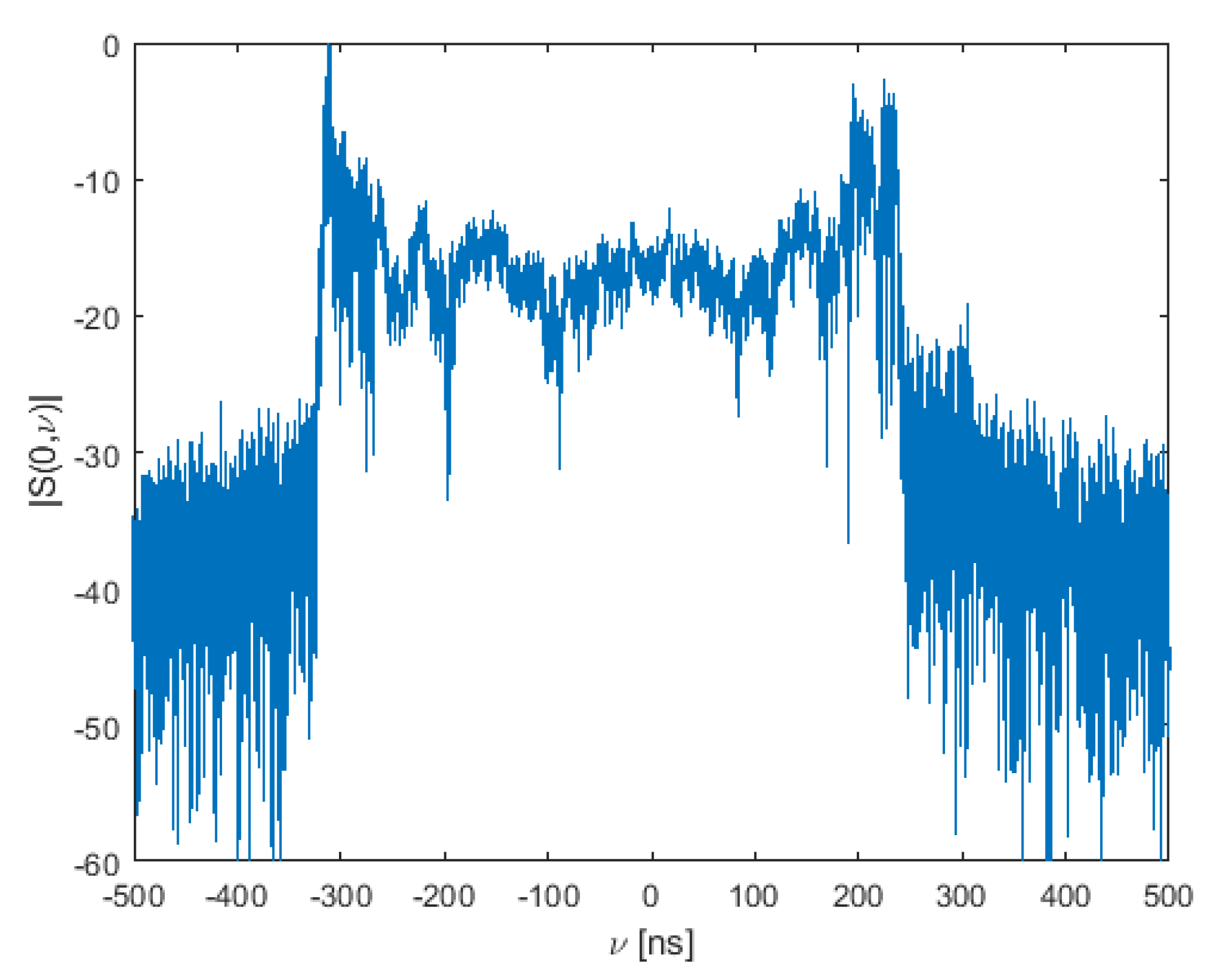
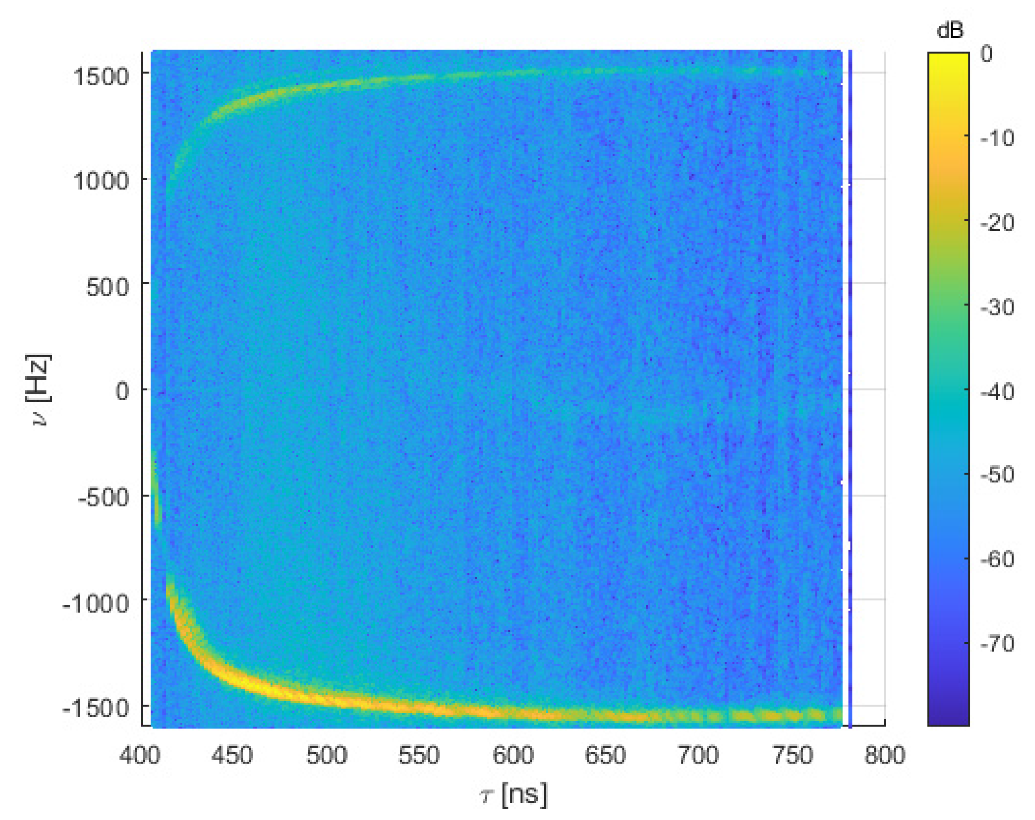
The delay-Doppler spectra, both for the received data and the samples aligned to the main component, are shown in Figure 23 and Figure 24. From the aligned responses, it can be derived that there is almost no multipath in the channel, which is consistent with what was previously exposed in this section. As we were moving away from the transmitter, it was expected that the main component would introduce a high Doppler shift in the negative frequencies.
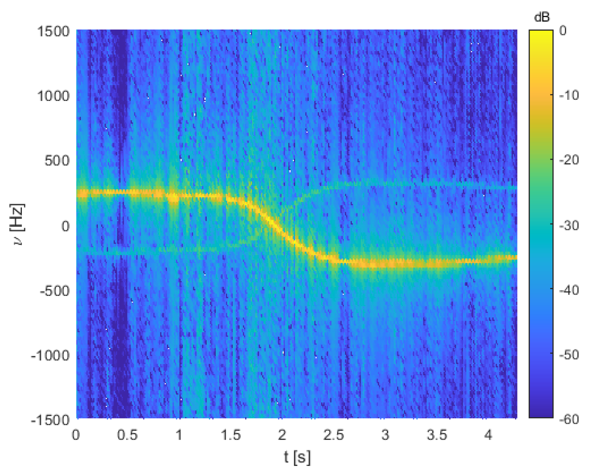
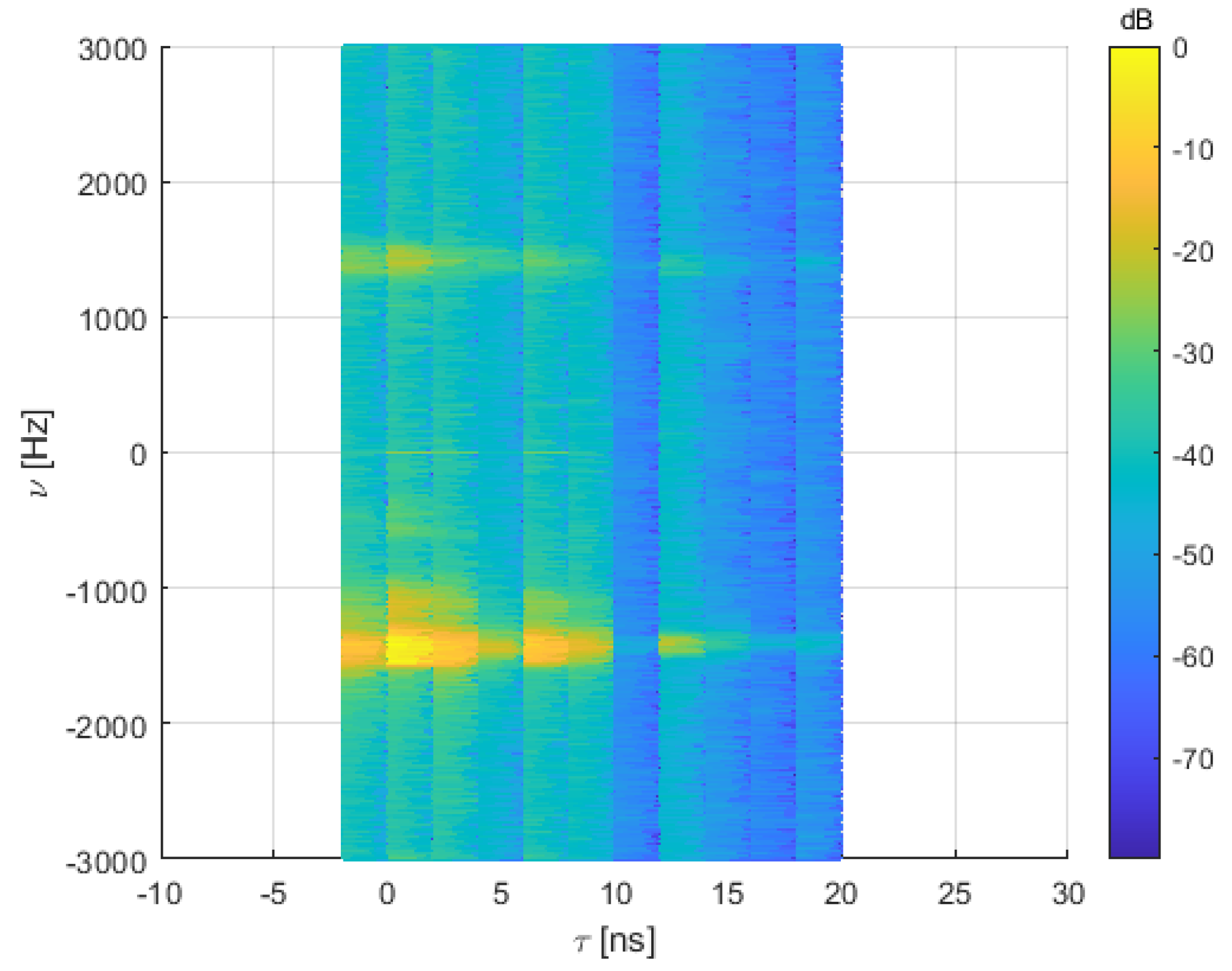
If we want to see how the Doppler spectrum associated to different delays varies with time, it is possible to repeat the procedure explained in the previous subsection. The result, again for an FFT size of 256, is shown in Figure 25. The variation of the Doppler spectrum as the vehicle moves can be appreciated clearly.
4. Discussion and Conclusions
The main result of this research is a wideband channel sounder especially suited for non-stationary channels. The compact size of the receiver eases transportation of the device and its installation on a vehicle. Multiple configuration changes can be done to best fit each measurement scenario. The current configuration of the sounder was given in Section 2.3. A list of possible configuration changes as well as their effects is now provided. Keep in mind that delay resolution is inversely related to sounding bandwidth, and maximum Doppler is half the channel-sampling rate.
- Chip rate. By configuration, slower clocks can be generated. This way, delay resolution and channel sampling rate are sacrificed to improve the length of a continuous measurement and the maximum unambiguous delay. Chip rate can be increased by using two converters. Currently, the FPGA boards used have two sockets for converters of the type FPGA Mezzanine Card (FMC). By using both, the chip rate can be doubled, but the deterministic latency described in the JESD204B interface protocol has to be implemented for synchronization [28]. Although the converters and synchronization algorithms were available during the previous campaigns, they were not used, so, at the moment, the maximum allowed chip rate is 500 Mchips/s. This rate gives the delay resolution of 2 ns and RF bandwidth of 1 GHz used in the tests.
- Averaging block size. The length of the averaging inside the FPGA can be modified in powers of 2, with a minimum length of 4 at the moment. Lesser order averages provide higher channel-sampling rates but cut down the duration of a full acquisition and vice versa. Further averaging can be performed offline for different purposes, as seen in Section 3.
- Channel-sounding sequence. It is easily interchangeable. Several of them can be preloaded and swapped without restarting the sounder. A number of options are available here. The simplest of these are to vary the order of the PRBS. Lesser order sequences increase channel-sampling rate at the cost of maximum delay and processing gain and vice versa. Currently, the maximum length for the sequences is 4096, half an FFT block.
- SDRAM depth. The DDR3 chip aboard the FPGA can be swapped by higher capacity models. These are inexpensive and allow to increase the amount of recorded channel responses in a single acquisition period.
Of course, changes related to the center frequency may be accomplished by means of swapping RF parts. In these cases, the core of the sounding system (FPGA plus converters) may still be used without any changes.
As explained in Section 1, a great number of channel sounders exist in the literature. Through the use of a frequency-domain conversion approach, we took advantage of pulse-compression techniques without requiring unfeasible or extremely complicated matched filters, as in the CMF architectures. We also avoided the use of sliding clocks to obtain CIRs, which would impact channel sampling period, as was the case of STDCC sounders.
A short channel-sampling period is quite important to characterize non-stationary channels like those of centimeter and millimeter wave systems. Several entities, such as academic institutions and research centers, have designed their sounders to accomplish this requirement. We believe that our proposal gives a combination of performance and cost that has not been achieved before. Many sounders based on commercial off-the-shelf (COTS) equipment and offline processing are capable of achieving great performance, but they have higher costs and a far more complicated maneuverability. This is the case of the sounders described in [15,16,17]. Although many of these kind of sounders are able to reach good bandwidths and channel measurement rates, their setup might be suboptimal in terms of cost and size. In contrast with the former, channel sounders with high flexibility and relatively low cost are presented in [18,24,29].
The sounder system described in [27] presents a great compromise between versatility, cost, and performance, being capable of achieving absolute timing. It counts with two modes: one based in STDCC and another similar to our approach. Nonetheless, our configuration is able to achieve similar characteristics in terms of the relation between delay resolution, Doppler bandwidth, and maximum continuous measurement time at lower costs, albeit without the absolute timing feature.
Author Contributions
Conceptualization, methodology, investigation, L.A.L.-V. and M.G.S.; data curation, L.A.L.-V.; writing—original draft preparation, L.A.L.-V. and M.G.S.; supervision, project administration, funding acquisition, M.G.S. All authors have read and agreed to the published version of the manuscript.
Funding
This research was funded by the Spanish Government, Ministry of Science and Innovation, under grants number TEC2017-85529-C3-3R and PID2020-112545RB-C52, Xunta de Galicia, grants ED431C 2019/26 and ED481A-2020/049 and the European Regional Development Fund (ERDF).
Data Availability Statement
Data are available on request due to restrictions. The data presented in this study are available on request from the corresponding author.
Acknowledgments
The authors would like to thank Isabel Expósito and Miguel Riobó for their assistance during the measurement campaigns. The authors would also like to thank Ignacio Boubeta as well for his valuable help in the assembly and set up of the hardware.
Conflicts of Interest
The authors declare no conflict of interest.
References
- Bello, P. Characterization of Randomly Time-Variant Linear Channels. IEEE Trans. Commun. Syst. 1963, 11, 360–393. [Google Scholar] [CrossRef] [Green Version]
- Rappaport, T.S. Wireless Communications: Principles and Practice, 2nd ed.; Prentice-Hall: Upper Saddle River, NJ, USA, 2002. [Google Scholar]
- Fleury, B.H. An uncertainty relation for WSS processes and its application to WSSUS systems. IEEE Trans. Commun. 1996, 44, 1632–1634. [Google Scholar] [CrossRef]
- Young, W.R.; Lacy, L.Y. Echoes in Transmission at 450 Megacycles from Land-to-Car Radio Units. Proc. IRE 1950, 38, 255–258. [Google Scholar] [CrossRef]
- Rees, J. Measurements of the wide-band radio channel characteristics for rural, residential, and suburban areas. IEEE Trans. Veh. Technol. 1987, 36, 2–6. [Google Scholar] [CrossRef]
- Cox, D. Delay Doppler characteristics of multipath propagation at 910 MHz in a suburban mobile radio environment. IEEE Trans. Antennas Propag. 1972, 20, 625–635. [Google Scholar] [CrossRef]
- Ferreira, D.; Caldeirinha, R.; Leonor, N. A Real Time High-Resolution RF Channel Sounder Based on the Sliding Correlation Principle. IET Microw. Antennas Propag. 2015, 9, 837–846. [Google Scholar] [CrossRef]
- Rappaport, T.S.; MacCartney, G.R.; Samimi, M.K.; Sun, S. Wideband Millimeter-Wave Propagation Measurements and Channel Models for Future Wireless Communication System Design. IEEE Trans. Commun. 2015, 63, 3029–3056. [Google Scholar] [CrossRef]
- Cid, E.L.; Sánchez, M.G.; Alejos, A.V. High speed transmission at 60 GHz for 5G communications. In Proceedings of the IEEE International Symposium on Antennas and Propagation & USNC/URSI National Radio Science Meeting, Vancouver, BC, Canada, 19–24 July 2015; pp. 1007–1008. [Google Scholar] [CrossRef]
- Lee, J.; Liang, J.; Kim, M.D.; Park, J.J.; Park, B.; Chung, H.K. Measurement-Based Propagation Channel Characteristics for Millimeter-Wave 5G Giga Communication Systems. ETRI J. 2016, 38, 1031–1041. [Google Scholar] [CrossRef]
- Miao, R.; Tian, L.; Zheng, Y.; Tang, P.; Huang, F.; Zhang, J. Indoor office channel measurements and analysis of propagation characteristics at 14 GHz. In Proceedings of the 2015 IEEE 26th Annual International Symposium on Personal, Indoor, and Mobile Radio Communications (PIMRC), Hong Kong, China, 30 August–2 September 2015; pp. 2199–2203. [Google Scholar] [CrossRef]
- Wu, T.; Rappaport, T.S.; Knox, M.E.; Shahrjerdi, D. A Wideband Sliding Correlator-Based Channel Sounder with Synchronization in 65 nm CMOS. In Proceedings of the 2019 IEEE International Symposium on Circuits and Systems (ISCAS), Sapporo, Japan, 26–29 May 2019; pp. 1–5. [Google Scholar] [CrossRef] [Green Version]
- Bajwa, A.S. Wideband Characterisation of UHF Mobile Radio Propagation in Urban and Suburban Areas. PhD’s Thesis, University of Birmingham, Birmingham, UK, 1979. [Google Scholar]
- Berger, G.L.; Safer, H. Channel sounder for the tactical VHF-range. In Proceedings of the MILCOM 97, Monterey, CA, USA, 3–5 November 1997; pp. 1474–1478. [Google Scholar] [CrossRef]
- Prokes, A.; Vychodil, J.; Mikulasek, T.; Blumenstein, J.; Zöchmann, E.; Groll, H.; Mecklenbräuker, C.F.; Hofer, M.; Löschenbrand, D.; Bernadó, L.; et al. Time-Domain Broadband 60 GHz Channel Sounder for Vehicle-to-Vehicle Channel Measurement. In Proceedings of the 2018 IEEE Vehicular Networking Conference (VNC), Taipei, Taiwan, 5–7 December 2018; pp. 1–7. [Google Scholar] [CrossRef]
- Papazian, P.B.; Gentile, C.; Remley, K.A.; Senic, J.; Golmie, N. A Radio Channel Sounder for Mobile Millimeter-Wave Communications: System Implementation and Measurement Assessment. IEEE Trans. Microw. Theory Tech. 2016, 64, 2924–2932. [Google Scholar] [CrossRef]
- Wen, Z.; Kong, H.; Wang, Q.; Li, S.; Zhao, X.; Wang, M.; Sun, S. MmWave channel sounder based on COTS instruments for 5G and indoor channel measurement. In Proceedings of the 2016 IEEE Wireless Communications and Networking Conference, Doha, Qatar, 3–6 April 2016; pp. 1–7. [Google Scholar] [CrossRef]
- Maharaj, B.T.; Wallace, J.W.; Jensen, M.A.; Linde, L.P. A Low-Cost Open-Hardware Wideband Multiple-Input–Multiple-Output (MIMO) Wireless Channel Sounder. IEEE Trans. Instrum. Meas. 2008, 57, 2283–2289. [Google Scholar] [CrossRef]
- Salous, S.; Feeney, S.M.; Raimundo, X.; Cheema, A.A. Wideband MIMO Channel Sounder for Radio Measurements in the 60 GHz Band. IEEE Trans. Wirel. Commun. 2016, 15, 2825–2832. [Google Scholar] [CrossRef] [Green Version]
- Pahlavan, K.; Howard, S.J. Frequency domain measurements of indoor radio channels. Electron. Lett. 1989, 25, 1645–1647. [Google Scholar] [CrossRef]
- Haneda, K.; Järveläinen, J.; Karttunen, A.; Kyrö, M.; Putkonen, J. Indoor short-range radio propagation measurements at 60 and 70 GHz. In Proceedings of the 8th European Conference on Antennas and Propagation (EuCAP 2014), The Hague, The Netherlands, 6–11 April 2014; pp. 634–638. [Google Scholar] [CrossRef]
- Riobó, M.; Hofman, R.; Cuiñas, I.; García Sánchez, M.; Verhaevert, J. Wideband Performance Comparison between the 40 GHz and 60 GHz Frequency Bands for Indoor Radio Channels. Electronics 2019, 8, 1234. [Google Scholar] [CrossRef] [Green Version]
- Shen, Y.; Shao, Y.; Xi, L.; Zhang, H.; Zhang, J. Millimeter-Wave Propagation Measurement and Modeling in Indoor Corridor and Stairwell at 26 and 38 GHz. IEEE Access 2021, 9, 87792–87805. [Google Scholar] [CrossRef]
- Keusgen, W.; Kortke, A.; Peter, M.; Weiler, R. A highly flexible digital radio testbed and 60 GHz application examples. In Proceedings of the 2013 European Microwave Conference, Nuremberg, Germany, 6–10 October 2013; pp. 740–743. [Google Scholar] [CrossRef]
- International Wireless Industry Consortium. Evolutionary & Disruptive Visions towards Ultra High. Capacity Networks White Paper; International Wireless Industry Consortium: Doylestown, PA, USA, 2014. [Google Scholar]
- Turing, G. An introduction to matched filters. IRE Trans. Inf. Theory 1960, 6, 311–329. [Google Scholar] [CrossRef] [Green Version]
- MacCartney, G.R.; Rappaport, T.S. A Flexible Millimeter-Wave Channel Sounder With Absolute Timing. IEEE J. Sel. Areas Commun. 2017, 35, 1402–1418. [Google Scholar] [CrossRef]
- Joint Electron Device Engineering Council (JEDEC). Serial Interface for Data Converters–JESD204B Standard. 2011. Available online: https://www.jedec.org/sites/default/files/docs/JESD204B.pdf (accessed on 29 June 2021).
- Seijo, Ó.; Val, I.; López-Fernández, J.A. Portable Full Channel Sounder for Industrial Wireless Applications With Mobility by Using Sub-Nanosecond Wireless Time Synchronization. IEEE Access 2020, 8, 175576–175588. [Google Scholar] [CrossRef]
Figure 1.
Transmitter configuration.

Figure 2.
Zenithal view of the receiver without its cover.

Figure 3.
Diagram of the transmitter.

Figure 4.
Diagram of the receiver.

Figure 5.
Scheme of the FPGA design at the receiver.

Figure 6.
Correlation of a repeating PRBS11 by the method proposed (FFT length = 8192, simulated channel response = δ(n) + 0.5·δ(n − 700)): (a) correlation of the periodical sequence without any changes; (b) output of a correlator, which is delayed by half an FFT block; (c) result after combining both outputs.

Figure 7.
Maximum Doppler shift produced at different carrier frequencies and relative speeds between Tx and Rx.
Figure 7.
Maximum Doppler shift produced at different carrier frequencies and relative speeds between Tx and Rx.

Figure 8.
Transmitter and receiver inside the laboratory.

Figure 9.
(a) Alley; (b) receiver mounted in the car for the tests in the alley.

Figure 10.
Transmitting antenna placed over the highway.

Figure 11.
Measured PDPs inside the laboratory.

Figure 12.
APDP inside the laboratory.

Figure 13.
Measured PDPs for the alley at low speeds (less than 25 km/h).

Figure 14.
Measured PDPs shifted to align the main component.

Figure 15.
APDP of the alley scenario.

Figure 16.
Delay spread in the alley: (a) variation along the measurement process; (b) CDF of the spread.
Figure 16.
Delay spread in the alley: (a) variation along the measurement process; (b) CDF of the spread.

Figure 17.
Delay-Doppler spectra from the alley campaign: (a) original data; (b) after aligning the responses with respect to the main path.
Figure 17.
Delay-Doppler spectra from the alley campaign: (a) original data; (b) after aligning the responses with respect to the main path.

Figure 18.
Doppler spectrum of the main component.

Figure 19.
Evolution of the Doppler spectrum of the main delay component.

Figure 20.
Measured PDPs at the alley at high speeds (120 km/h).

Figure 21.
Measured PDPs shifted to align the main component.

Figure 22.
Delay spread in the highway: (a) variation along the measurement process; (b) CDF of the spread.
Figure 22.
Delay spread in the highway: (a) variation along the measurement process; (b) CDF of the spread.

Figure 23.
Delay-Doppler spectra from the highway campaign without aligning the main contribution.

Figure 24.
Delay-Doppler spectrum computed from the aligned samples.

Figure 25.
Evolution of the Doppler spectrum of the main delay component.


Table 1.
Hardware components of the transmitter.
| Block | Function | Component |
|---|---|---|
| FPGA | Sequence generator | Xilinx VC707 |
| DAC | DAC | AD9161-FMCC-EBZ |
| Rubidium | Frequency reference | SRS PRS10 |
| LO | Local oscillator | HP 83650B |
| Multiplier | Mixer | MITEQ M1826W1 |
| Amplifier | Power amplifier | ERZ-HPA-2700-4200-27 |
| Antenna | Omnidirectional antenna | Flann 21240-20 |
| Directional antenna | MD249-8193 |
Table 2.
Hardware components of the receiver.
| Block | Function | Component |
|---|---|---|
| FPGA | Correlator | Xilinx VC707 |
| ADC | ADC | AD-FMCADC3-EBZ |
| LPF | Anti-aliasing filter | Mini-Circuits SLP-1200+ |
| Multiplier | Mixer | MITEQ DB0440HW1-R |
| Band-pass filter | Band selector | Knowles B280LB0S |
| Amplifier | Low-noise amplifier | MITEQ AMF-5F-26004000-25-13P |
| Antenna | Antenna | Flann MD249-8193 |
| Rubidium | Frequency reference | SRS PRS10 |
| 2 GHz LO | Phase-Locked Loop (PLL) | EMF Systems 52747-443024 |
| 14 GHz LO | PLL | MITEQ DLCRO-010-14075-4-12P |
| Frequency multiplier | Frequency multiplier | MITEQ MAX2M200400-20P |
Table 3.
Sounder performance.
| Parameter | Value |
|---|---|
| Carrier frequency | 28.65 GHz |
| RF Bandwidth | 1 GHz |
| Delay resolution | 2 ns |
| Channel excitation signal | PRBS-11 |
| Maximum unambiguous delay | 4.09 µs |
| Channel sampling frequency | 15.27 kHz |
| Maximum Doppler shift | 7.63 kHz |
| Maximum sounder speed at fc | 287.74 km/h |
| Maximum continuous acquisition interval | 4.29 s |
| Channel samples per full measurement cycle | 65,536 |
| Processing gain | 33.11 dB |
| Dynamic range | 57 dB |
Table 4.
Comparison between measured and computed Doppler shift.
| t (s) | v (m/s) | α (º) | νth (Hz) | νmeas (Hz) |
|---|---|---|---|---|
| 0 | 5.05 | 62.5 | 222.69 | 223.6 |
| 1 | 5.75 | 66.5 | 218.96 | 223.6 |
| 2 | 7.27 | 97.5 | −90.62 | −89.45 |
| 3 | 7.30 | 117.0 | −316.50 | −313.1 |
| 4 | 5.34 | 124.0 | −285.17 | −283.3 |
Publisher’s Note: MDPI stays neutral with regard to jurisdictional claims in published maps and institutional affiliations. |
© 2021 by the authors. Licensee MDPI, Basel, Switzerland. This article is an open access article distributed under the terms and conditions of the Creative Commons Attribution (CC BY) license (https://creativecommons.org/licenses/by/4.0/).
Share and Cite
MDPI and ACS Style
López-Valcárcel, L.A.; García Sánchez, M. A Wideband Radio Channel Sounder for Non-Stationary Channels: Design, Implementation and Testing. Electronics 2021, 10, 1838. https://doi.org/10.3390/electronics10151838
AMA Style
López-Valcárcel LA, García Sánchez M. A Wideband Radio Channel Sounder for Non-Stationary Channels: Design, Implementation and Testing. Electronics. 2021; 10(15):1838. https://doi.org/10.3390/electronics10151838
Chicago/Turabian StyleLópez-Valcárcel, Luis A., and Manuel García Sánchez. 2021. "A Wideband Radio Channel Sounder for Non-Stationary Channels: Design, Implementation and Testing" Electronics 10, no. 15: 1838. https://doi.org/10.3390/electronics10151838
Note that from the first issue of 2016, this journal uses article numbers instead of page numbers. See further details here.