
Wavelet Threshold Ultrasound Echo Signal Denoising Algorithm Based on CEEMDAN

1
School of Electrical Engineering and Automation, Tianjin University of Technology, Tianjin 300384, China
2
CNOOC Enertech Equipment Technology Co., Ltd., Tianjin 300452, China
*
Author to whom correspondence should be addressed.
Electronics 2023, 12(14), 3026; https://doi.org/10.3390/electronics12143026
Submission received: 31 May 2023
/
Revised: 6 July 2023
/
Accepted: 7 July 2023
/
Published: 10 July 2023
(This article belongs to the Special Issue Signal Processing, Sensor Fusion, and Data Fusion in Measurement Systems)
Abstract
:In this study, an algorithm for denoising ultrasound echo signals in industrial settings is proposed to address the problem of high noise and low signal-to-noise ratio. The algorithm combines complete ensemble empirical mode decomposition with adaptive noise (CEEMDAN), mutual information entropy (MIE), and wavelet threshold denoising to ensure effectiveness given the unique structure of ultrasound echo signals. Initially, CEEMDAN is used to decompose the signal into intrinsic mode function (IMFs) and residual signals. The MIE is then used to determine the correlation of neighboring IMF signals, which are then divided into a noise- and a signal-dominated part. Finally, using wavelet thresholding, noise is suppressed in the signal-dominant part, and the resulting denoised signal is reconstructed using the residual signal. The performance of the algorithm is verified through simulations and physical experiments, and the results show that it is superior to traditional signal denoising methods.
1. Introduction
Ultrasonic waves are non-linear physical signals [1] consisting of high-frequency mechanical waves that propagate easily. Due to their high penetrative power [2], the use of these waves has become an essential aspect of modern technological applications. Ultrasonic technology employs the vibrations caused by high-frequency sound waves to realize detection or processing, and it is gaining increasing importance in fields such as medicine [3], industry [4], materials [5], and environmental [6] protection. Owing to its non-hazardous nature to humans [7], ultrasound technology is widely utilized in the medical and industrial sectors, while non-destructive testing with ultrasonic waves has become an established and popular method [8,9]. Due to these characteristics, ultrasound technology will further advance and shape the progress and development of science and technology. Therefore, the accurate estimation of ultrasonic echo signals is crucial for obtaining precise echo information, particularly in applications with high measurement accuracy requirements.
Several scholars have proposed different calculation methods for analyzing ultrasonic echo signals, including the optimization of transducer models [10], analysis of echo signal spectra [11], and modeling of echo signal parameters [12]. Effective noise reduction is a crucial prerequisite for the accurate analysis of ultrasonic echo signals using various analysis methods [13]. The conventional contemporary method for filtering ultrasonic echo signals involves the use the concepts of Fourier and wavelet transforms. Nevertheless, Fourier transform only suits stable-frequency signals without details of the embodied signal, as it is based on sine functions and delivers a comprehensive transformation [14]. On the contrary, wavelet transform is more suitable for analyzing unstable ultrasonic echo signals for the presence of specific components [15]. However, the limited ability to generalize hinders its practical application. Empirical mode decomposition (EMD) outperforms wavelet transform when dealing with non-periodic and non-stationary signals, but results in modal aliasing in the intrinsic mode functions (IMFs) obtained [16,17]. Ensemble empirical mode decomposition (EEMD) mitigates modal aliasing through the introduction of white noise to the input signal, repeated application of EMD, and averaging of the results [18]. Despite this, some residual white noise remains in the final reconstructed signal. Complementary ensemble empirical mode decomposition (CEEMD) is used to reduce the effects of modal aliasing by introducing positive and negative white noise perturbations into the original signal, decomposing the signal with EMD, and finally averaging the results of multiple decompositions [19]. However, its IMF components are difficult to align in the final ensemble averaging. The complete ensemble empirical mode decomposition with adaptive noise (CEEMDAN) was introduced to address these difficulties [20]. CEEMDAN employs adaptive white noise to address the problems of high-to-low frequency transfer of white noise and IMF alignment, and has shown excellent completeness [21].
In this study, the CEEMDAN algorithm is first used to decompose the acoustic signal into several IMFs and residues. The result is then partitioned into components dominated by noise and the signal itself based on the mutual information entropy (MIE) of the IMFs. A modified wavelet threshold method is applied to reduce the level of noise in the dominant part of the signal. This results in a denoised signal, which is then reconstructed along with the residual signal. Through simulation and the evaluation of actual measurement data, the signal-to-noise ratio (SNR) and other indicators, including the root-mean-square error (RMSE), show that this algorithm has superior noise reduction capabilities compared to traditional processing methods.
The remaining contents of this article are as follows. The ultrasonic Gaussian echo model is described in Section 2, and algorithmic framework and principles of the system are presented in Section 3. The simulation and physical experiments are discussed in Section 4 and Section 5, respectively. Finally, the conclusions and outlook of the proposed system are given in Section 6.
2. Establishing Ultrasonic Echo Signal Model
The most commonly used transducer in the application of ultrasound detection is the piezoelectric transducer. The ideal ultrasonic echo signal exhibits Gaussian random characteristics, i.e., the envelope follows a Gaussian distribution [22,23]. The mathematical models used to analyze ultrasonic signals received by transducers mainly consist of the Gaussian model, the double Gaussian attenuation model, and the asymmetrical Gaussian model [12]. These models are widely adopted in the numerical analysis of ultrasonic signals. The functional description of the Gaussian model is as follows:
In this equation, represents the Gaussian model, while the model parameter comprises five different vectors that have intuitive meanings: is the ultrasonic echo amplitude , is the bandwidth factor , is the delay time , is the center frequency , and is the phase . In practical applications, ultrasonic signals are subjected to varying degrees of noise. Thus, during simulations, different levels of Gaussian white noise need to be incorporated so that the resulting signal constitutes a realistic simulation of real-life scenarios. The ultrasonic echo model can be therefore be defined as:
In this equation, denotes the ultrasonic echo signal degraded by noise and is defined as the random Gaussian white noise.
3. Method for Analysis of Echo Signals
In this section, a brief introduction to three signal feature analysis methods is first provided: CEEMDAN decomposition, MIE extraction, and the improved wavelet threshold denoising algorithm. Subsequently, we will explain the algorithm for analyzing the ultrasonic echo signals proposed in this paper.
3.1. CEEMDAN
EMD involves the decomposition of a non-smooth signal into IMFs components and residual components [24]. Each IMF represents the intrinsic vibration mode of the signal at a particular time or time–frequency scale, which reflects the flow characteristics of the signal at different time scales, and can be used for local analysis of the signal. EMD decomposes the signal using the following equation:
Here, the input signal is represented using , where , denotes the IMF component, and . Furthermore, denotes the residual component.
Although EMD is commonly used for the decomposition of non-smooth signals, it suffers from modal mixing. To solve this problem, Huang et al. [25] proposed a new time-frequency analysis method, EEMD. EEMD is based on the EMD method and introduces randomization processing and integration methods to overcome the shortcomings of EMD. However, EEMD still has some drawbacks. For example, the decomposition process of a composite signal is independent and they are not linked, which can lead to incomplete decomposition [26]. To overcome the drawbacks of EEMD, the CEEMDAN algorithm was proposed by Torres et al. [20]. In this algorithm, reconstruction errors are gradually eliminated through the adaptive addition of while noise to each signal decomposition level, thus reducing mode mixing, while ensuring the effectiveness of the signal decomposition [27]. The first step of the method presented in this paper is the application of CEEMDAN for the decomposition of the ultrasonic echo signal.
Step 3.1.1. The noise-containing ultrasound echo signal undergoes processing through the addition of a Gaussian white noise signal , where represents the number of groups with Gaussian white noise added. This process results in the composite signal , which is the sum of the addition of noise and the original signal:
Step 3.1.2. The resulting composite signals are decomposed using EMD and the first modal IMF components obtained from all decompositions are averaged. This is taken as the first IMF of the CEEMDAN decomposition, and is expressed through the following equation:
Step 3.1.3. The residual signal is updated based on obtained from the previous step.
Step 3.1.4. is defined as the q-th of the EMD signal. is added to the residual signal to obtain a new signal, to which EMD is then applied. The first IMF components of these decompositions are then averaged to obtain the second of CEEMDAN:
Step 3.1.5. The residual component of the second is calculated as:
Step 3.1.6. The updated residual signal undergoes iterative decompositions according to the processes defined in Steps 3.1.4 and 3.1.5 until it cannot be further decomposed. The intrinsic mode components are obtained, in total, along with the final residual signal . The processed ultrasound echo signal can then be expressed using the following equation:
The components obtained via CEEMDAN are sequenced and sorted according to their spectral frequencies from high to low, with each representing the spectral amplitude contribution proportion present within distinct frequency bands of the signal.
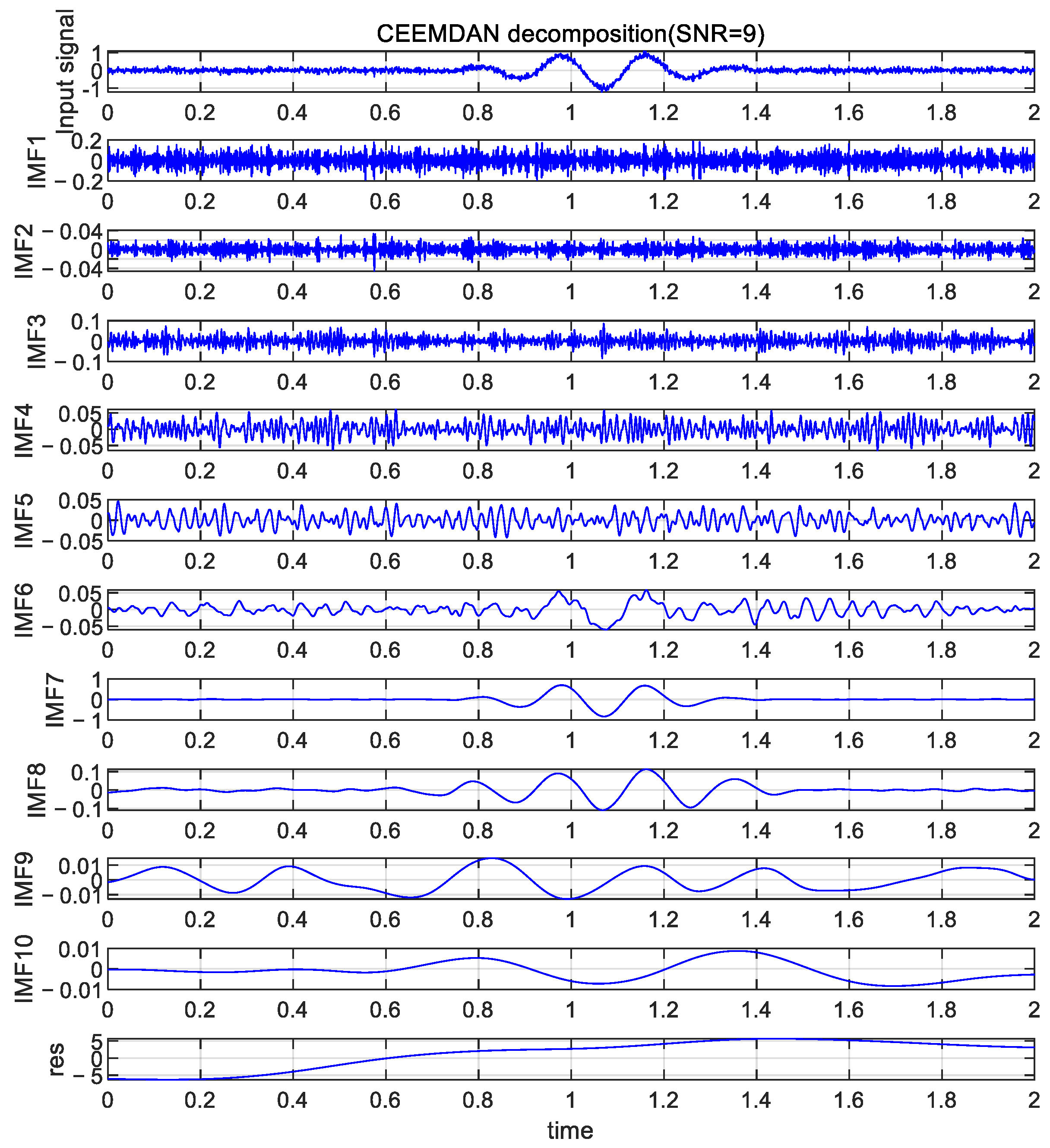
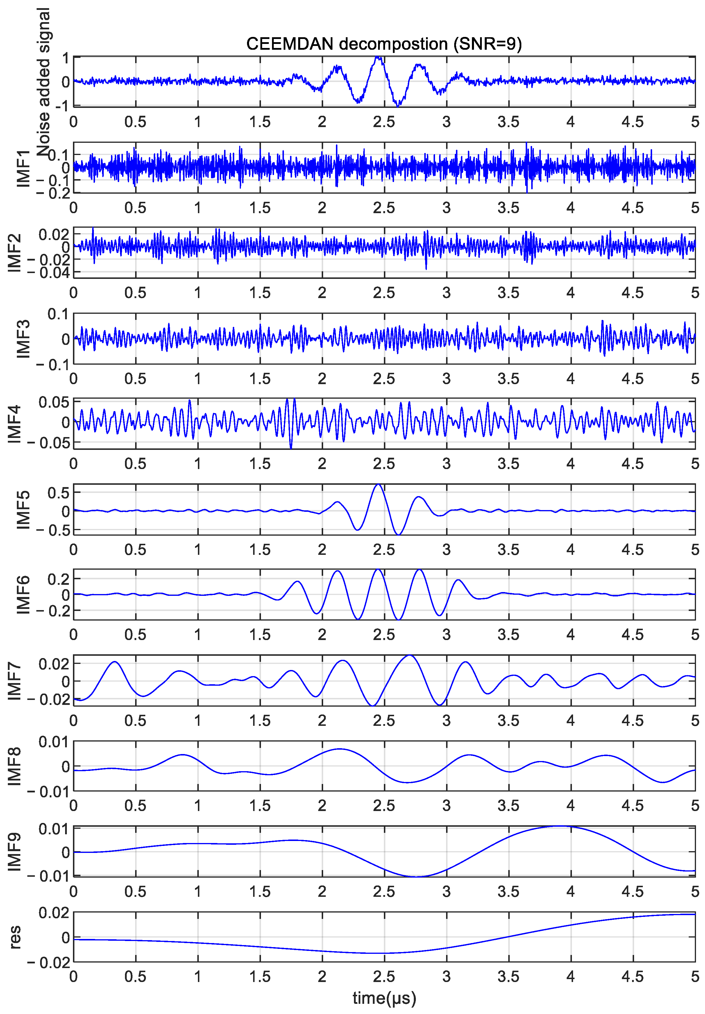
Using the parameters of the ultrasonic echo Gaussian model from [22], the resulting Gaussian model is shown in Figure 1. A Gaussian white noise was added to Figure 1 and decomposition was then performed using the CEEMDAN algorithm described in this section to obtain the IMF and residual components at different frequency bands. The decomposition is shown in Figure 2.
3.2. Mutual Information Entropy
MIE is a dimensionless statistic used to measure the amount of information that a random variable can provide about changes in another random variable [28]. It reflects the amount of information that the random variables contain about each other, or their statistical interdependence. The signal is decomposed using CEEMDAN to obtain K IMF components, where the set of IMFs that contribute more to the original signal is considered as the dominant part of the signal, while IMFs that contribute little to the original signal, which are mainly composed of high frequency noise, are defined as the noise-dominated part. Since CEEMDAN addresses the modal mixing phenomenon of IMF, it can be assumed that the noise-dominated part does not contain the characteristics of the signal analyzed. Therefore, the boundary between the noise- and signal-dominated parts must be found, and the noise-dominated part is discarded before the signal-dominated part is processed. From the properties of the MIE, it can be seen that a higher MIE corresponds to a greater degree of correlation between two random variables and more, mutual information. When two random variables are independent and uncorrelated, their MIE value is zero [29]. Therefore, it can be assumed that the high and the low frequency components are partially statistically independent of each other. When calculating the MIE of adjacent IMFs, the local minimum is used as the dividing point between the high and low frequency components [30]. If is set to be the q-th IMF component IMFq, , and is the valid IMF signal adjacent to , then the MIE algorithm is implemented as follows:
Step 3.2.1. Divide the time interval of equally into m groups, each of length 1/m. From the definition and the equation of the information entropy, it follows that:
where is the marginal probability distribution.
Step 3.2.2. Similarly, find the information entropy of .
Step 3.2.3. The joint distribution entropy is obtained from the definition of information entropy as:
where is the joint probability distribution.
Step 3.2.4. The MIE between the random variables and is:
Written in collated from, this gives:
It is therefore possible to find the MIE for each neighboring IMF.
3.3. Wavelet Thresholding Denoising Method
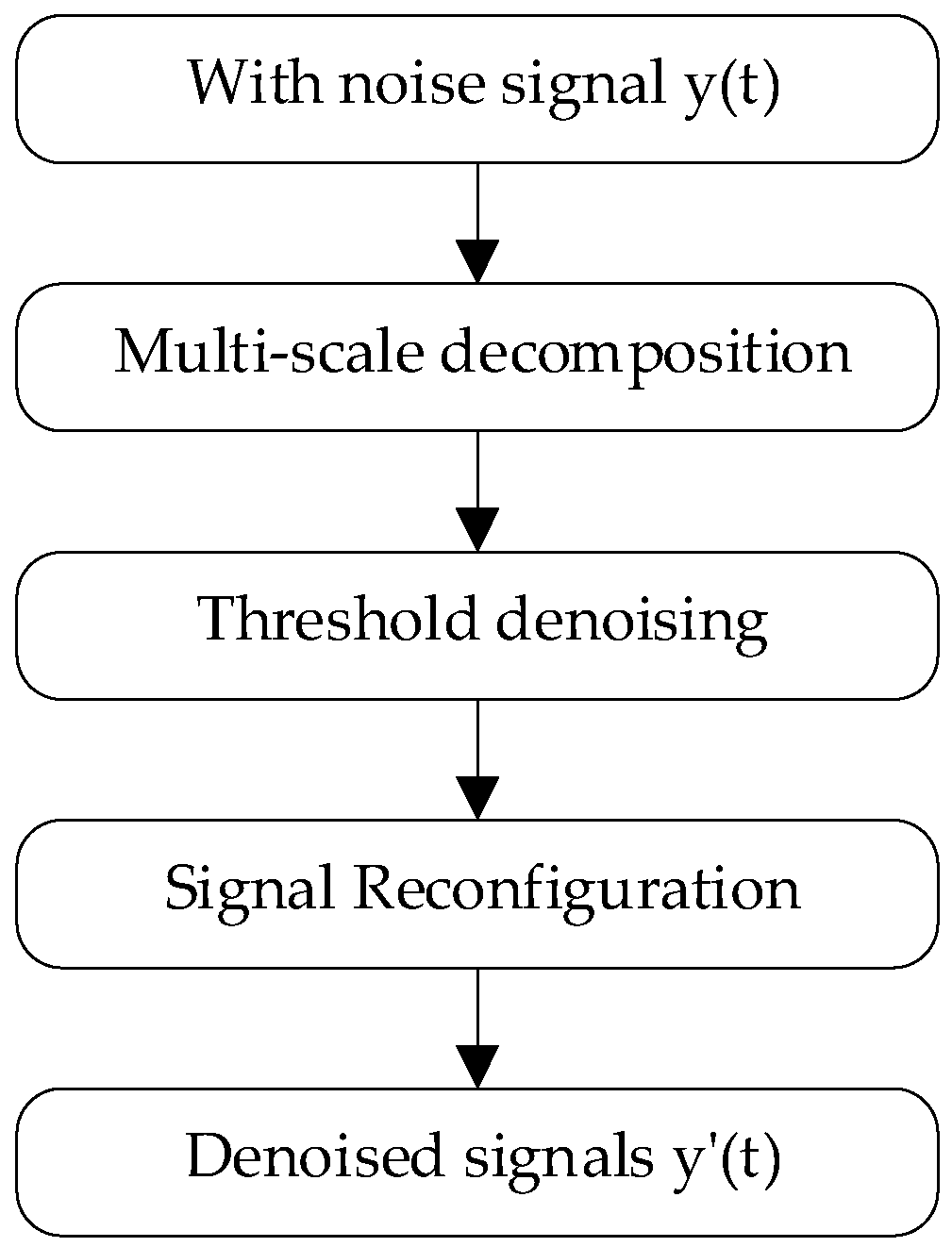
Wavelet transformation is a commonly utilized multiscale information analysis method with excellent denoising capabilities, which has resulted in its widespread adoption in different applications. The wavelet threshold denoising process flowchart is as shown in Figure 3:
The following steps can be taken to achieve wavelet decomposition of the signal:
Step 3.3.1. In Equation (14), represents the signal with noise, contains the useful signal comprising the low-frequency information, and represents the high-frequency noise signal. is then further decomposed to generate scale and wavelet coefficients for each layer.
Step 3.3.2. An appropriate wavelet basis and decomposition layers are selected to perform the multiscale wavelet decomposition of the noise signal and obtain the wavelet coefficients .
Step 3.3.3. Choosing an appropriate threshold function is critical for effective wavelet threshold denoising. The two most common threshold methods, namely, hard and soft thresholding, were proposed by Donoho and Johnstone [31] and both remove various types of noise from the signal. This noise can interfere with the signal’s characteristic information, making signal processing difficult, especially during the transmission process. Although the ideal ultrasound signal is a stationary Gaussian random process, in practical terms, the signals are non-stationary due to the influence of the measurement environment and medium. In this paper, CEEMDAN decomposition of the ultrasonic echo signal is applied, where the MIE classification is used to discard the noise-dominant parts of the process. This is similar in function to a low-pass filter, which only suppresses the high-frequency noise in the original signal and does not take into account the noise in the dominant part of the signal. Therefore, selecting a reasonable threshold function is crucial for suppressing noise in the dominant part of the signal.
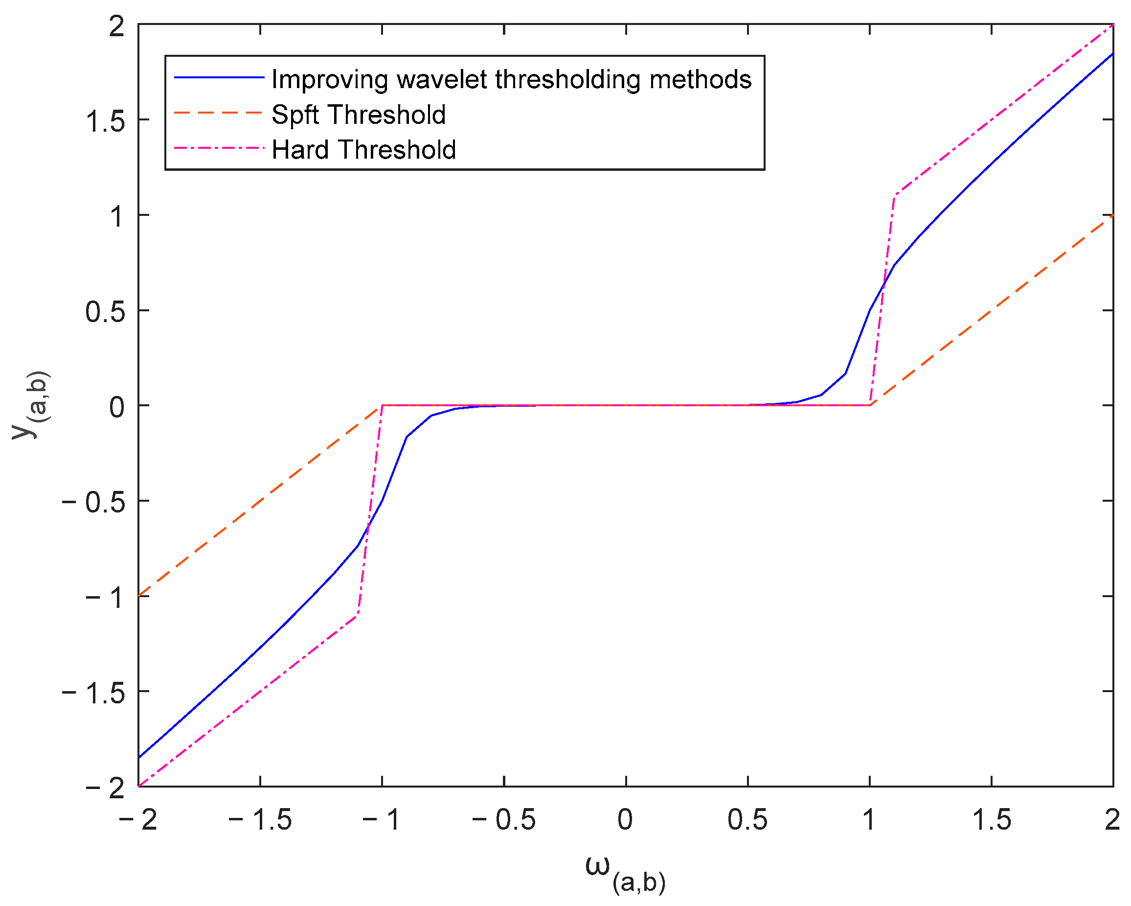
The hard thresholding method is particularly suitable for denoising signals with dispersed energy, as it directly removes any coefficients and noise below the specified threshold. However, this method has a disadvantage in that the threshold result may be discontinuous, producing additional oscillations. The soft thresholding method is often used for signals with relatively concentrated energy, better preserving the smoothness and continuity of the signal. However, it may lead to loss of signal detail and blurring. For this study, a custom threshold function was utilized for improved wavelet threshold denoising, as described in [32]. This method involves the smoothing of the wavelet threshold location to enhance the denoising effect. The threshold function is expressed as follows:
where is the output wavelet coefficient, is the input wavelet coefficient, is the signum function, and and are the threshold function adjustment factors, where . In the paper, and . The improved threshold function and the hard the soft threshold function curves are plotted against each other.
As shown in Figure 4, the improved thresholding function overcomes the problem of fixed deviation values for soft thresholding and improves the abruptness present in the hard thresholding function at , which results in a better denoising effect.
Step 3.3.4. The threshold is also a very important parameter, and the fixed threshold function is defined as:
In the above equation, is the standard deviation of the noise, is the median operator, and is the sample length of the noisy signal.
Step 3.3.5. The processed wavelet coefficients are used for the reconstruction process and finally to obtain the wavelet threshold denoised signal .
3.4. Echo Signal Estimation Method
The proposed algorithm of the present study analyzes the echoic ultrasound echo signal based on the theory explained above. The complete process is shown in Figure 5.
Step 3.4.1. Assume that the input signal of the noise-laden ultrasound echo is . The signal is first decomposed using the CEEMDAN algorithm to produce components (, ,..., ) and the corresponding residual information . The components are arranged in descending order of frequency, with high-frequency noise primarily forming the low-order . Conversely, high-order primarily include low-frequency noise and the signal components of the original signal. The MIE is then used to calculate the correlation between adjacent :
Step 3.4.2. The cut-off point is then determined through the calculation of the MIE values of the adjacent and finding the local minimum. The components are decomposed into noise-dominated components and signal-dominated components . The expressions for the cut-off points and signals are as follows:
Step 3.4.3. In order to remove the low-frequency noise components found in the dominant part of the signal, wavelet threshold denoising is applied to this part. The resulting denoised signal, , is then combined with the residual signal, , to produce a new signal, , that is calculated using the following equation:
4. Simulation Experiments
4.1. Simulation Experiment Platform
In order to evaluate the impact of the proposed algorithm on ultrasonic echo signal analysis, ultrasonic echo signals were synthesized using the Gaussian model. The experimental platform used has a Windows 11 operating system with a Ryzen six-core R5-6600H processor, 16.0GB of memory, and an RTX3050 4Gb discrete graphics card. The model simulation experiments were conducted using MATLAB. The feasibility and effectiveness of the CEEMDAN algorithm combined with the wavelet threshold denoising algorithm for ultrasonic echo signal processing were verified for the simulated Gaussian model-based signals. This ultrasonic echo signal model was established using known parameters, providing a suitable test framework.
The simulations were performed using the ultrasonic Gaussian model Equation (1) as the reference signal, as shown below:
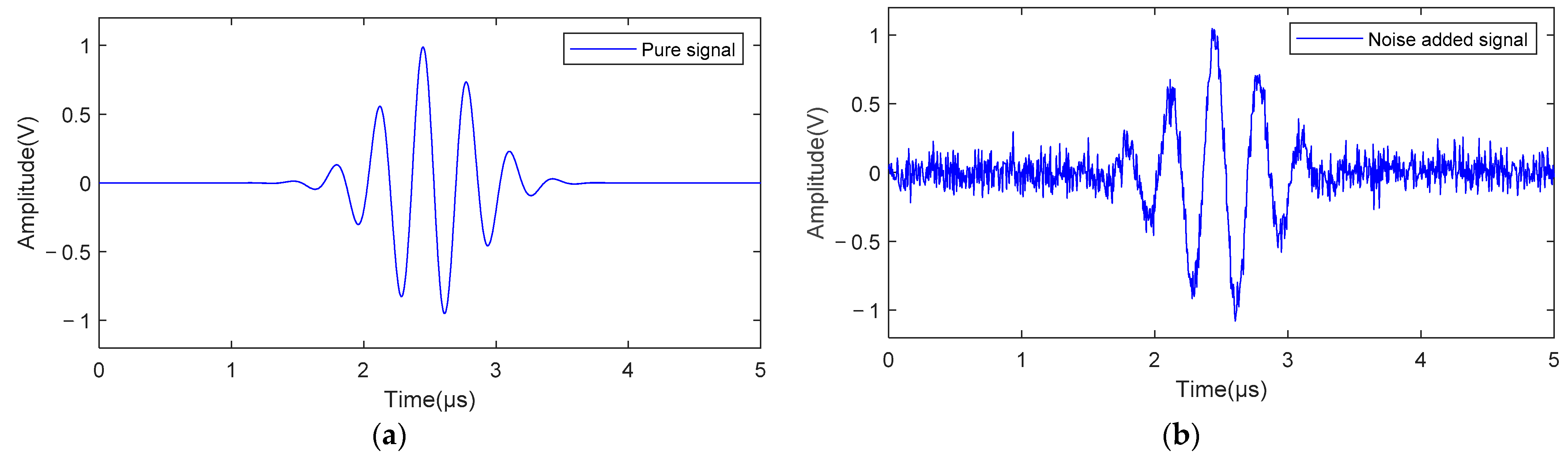
In this section, the proposed method is employed to process the simulated signal to demonstrate its validity. The discretized sample, , was obtained using a sampling interval of , samples, and a total waveform duration of . Following Equation (2), zero-mean Gaussian white noise was added to the reference signal to simulate the external disturbances typically encountered in practical applications, and the original signal was replaced by the disturbed signal . Signal sequences with an SNR of 0–30 dB were generated using different , and simulation experiments were performed to verify the proposed scheme.
4.2. Evaluation Index
Several metrics were utilized to assess the algorithm’s denoising performance. These metrics included the , , and normalized cross-correlation (). Let denote the reference signal of the Gaussian model, and represent the denoised signal, while represents the length of the signal.
The equation for is as follows:
The equation for RMSE is as follows:
The equation for is as follows:
4.3. Simulation Result
Figure 6 illustrates the echo signal simulation generated using a Gaussian model. The time-domain graph of the pure ultrasonic echo signal is displayed in Figure 6a, while the time-domain graph of the noisy signal with an SNR ratio of 9 dB is shown in Figure 6b.
The CEEMDAN method was employed as a first step to decompose the noisy signal into multiple IMF components and residue signals. The decomposed signal’s structure is illustrated in Figure 7.
Figure 7 illustrates that IMF1 to IMF4 represent high-frequency signals, while IMF5 to IMF9 depict low-frequency signals. Each IMF contains specific information about the signal. However, not all signal decompositions differentiate between the signal- and noise-dominated boundaries effectively. The results of calculating the adjacent IMF signals using MIE are shown in Table 1. At this point, means that the MIE of IMF4-5 is a local minimum, so it can be concluded that IMF1–IMF4 constitute the noise-dominated part and IMF5–IMF9 contain the signal-dominated part.
The signal-dominated part from IMF5 to IMF9 was reconstructed. It can be seen from Figure 8 that some noise still remained in the signal-dominated part, which was removed using wavelet thresholding during the next step.
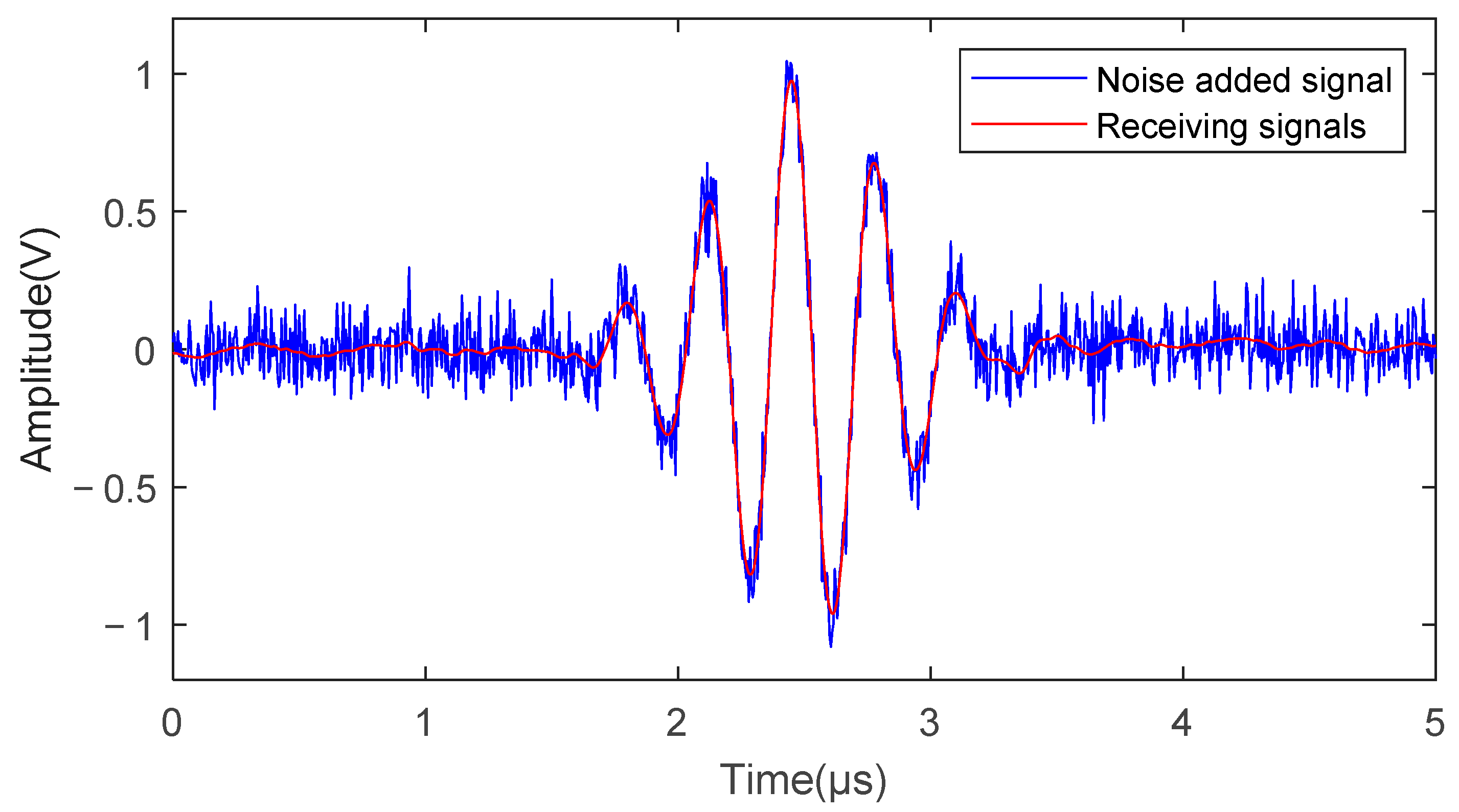
The signal-dominated part was denoised in the improved wavelet thresholding method using reasonable wavelet bases and threshold functions. In this paper, the threshold function selected was obtained from [32] for processing and the coif5 wavelet base function was adopted; the general thresholding method (visushrink) was used for denoising. The comparison between the denoised signal and the reconstructed version of the residual signal obtained from CEEMDAN decomposition and the original signal is shown in Figure 9.
To validate the efficacy of the proposed algorithm for noise reduction, its performance was evaluated based on the SNR, RMSE, and NCC, as illustrated in Table 2.
From Table 2, it is evident that at maximum noise interference levels, the SNR is 0 dB. The proposed denoising algorithm improved the SNR up to 12.6890 dB, while maintaining an RMSE of 0.058 and an NCC of 0.974. At lower noise levels, such as when the SNR was 30 dB, the corresponding denoising values achieve were 37.4580, 0.0033, and 0.99992. Thus, it can be inferred that the similarity between the received signal and the pure signal increases through the application of the proposed denoising algorithm.
To conduct further comparisons of the noise reduction effects of different methods under identical noise levels, a comparison of the traditional algorithms was conducted using an original signal with an SNR of 9 dB, as demonstrated in Table 3. Based on the three evaluation criteria, it is evident that the denoising algorithm presented in this study had the highest SNR and NCC values for the reference signal, as well as the lowest RMSE. Therefore, it can be concluded that the proposed algorithm exhibits superior performance.
A further comparison was conducted with several advanced research methods, as shown in Table 4. The experiments were performed with a signal-to-noise ratio of 10 dB and Gaussian model parameters using B, i.e., . Group C refers to the method presented in this paper. The results show that the denoising algorithms in this paper have a higher SNR, lower RMSE, and better denoising effect compared to other algorithms.
5. Physical Experiments
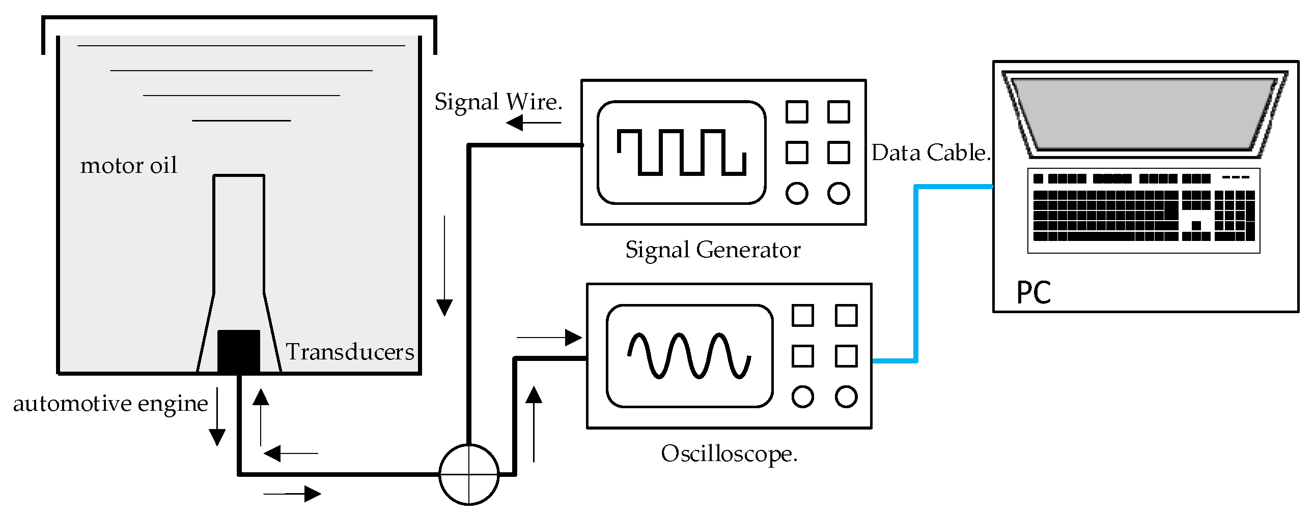
In this section, the algorithm’s performance is verified through its application in measuring an engine’s oil level. The engine oil level is a critical parameter that affects automobile operation. Ultrasonic oil level gauges operate on the principle of measuring the propagation time of ultrasonic waves in the oil and estimating ultrasonic echo signals. The experimental setup for measuring the oil level included an integrated immersion ultrasonic transducer, a pulse generator, a digital oscilloscope, an oil tank, a high-speed switch, and a computer. Figure 10 shows the schematic diagram of the system.
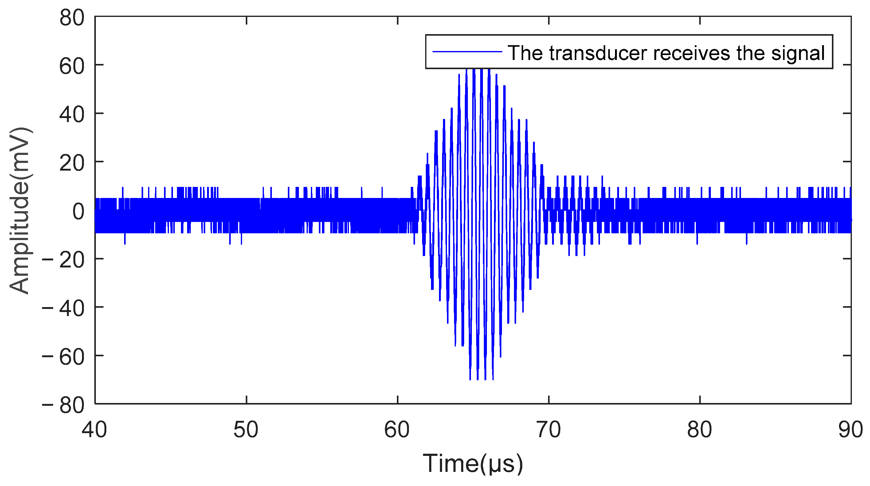
The signal generator produced pulses that drove the transducer to generate ultrasonic waves. The ultrasonic signal, propagated through the oil medium, was reflected by the oil surface, received and converted into an electrical signal by the transducer, and, finally, collected using the oscilloscope. The oscilloscope had a sampling frequency of 1 GHz, collecting 50,000 data points at intervals of 0.001 . Figure 11 displays the original echo signal, indicating the presence of high-frequency noise before 60 and after 75 .
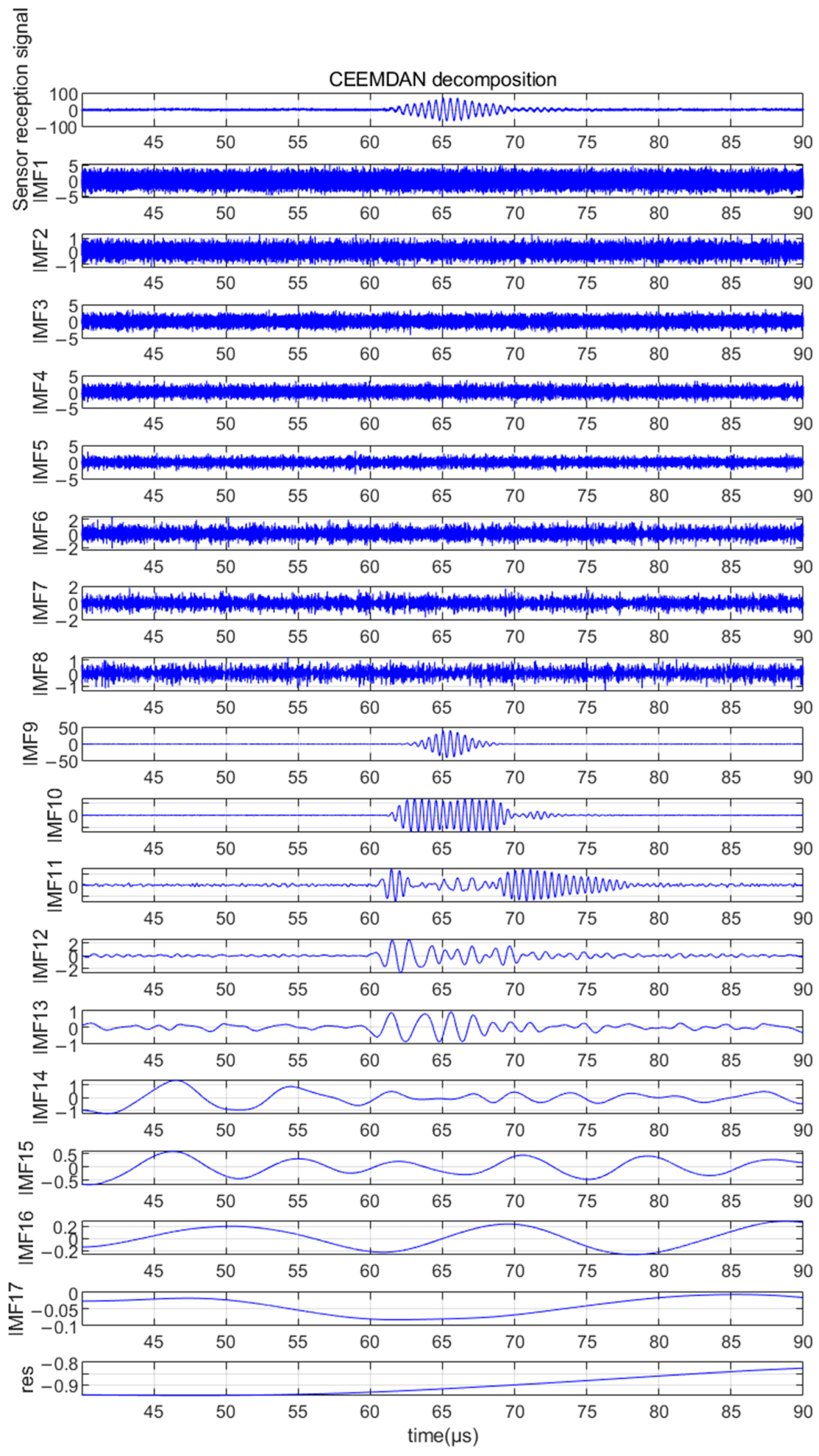
The raw signal received by the sensor was decomposed using CEEMDAN, which yielded 16 IMF components and one residual signal, as shown in Figure 12.
As shown in Table 5, the MIE of IMFs 8–9 were local minima and therefore IMF1–IMF8 were considered the noise-dominated part and discarded. IMF9–IMF16 constituted the signal-dominated part.
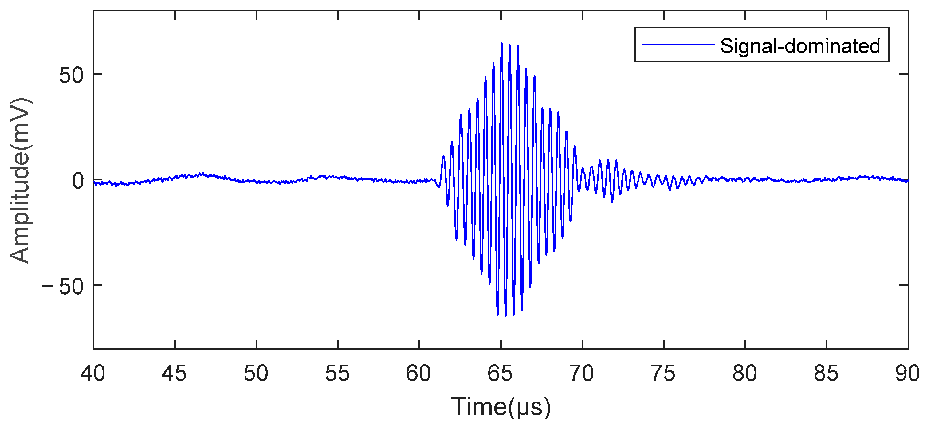
Therefore, IMF9–IMF17 were reconstructed to obtain the signal dominant portion, as shown in Figure 13. It can be seen that there was still some noise in the signal-dominated portion.
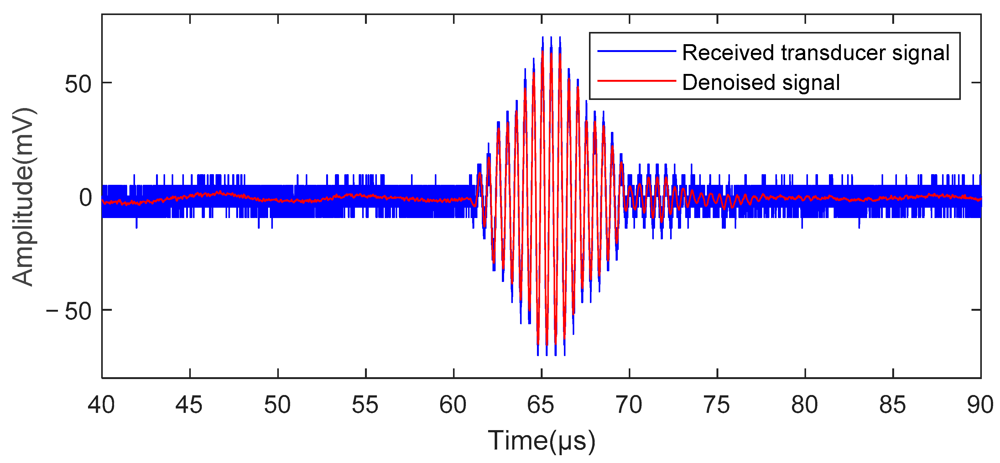
The curves shown in Figure 14 were obtained via processing the dominant part of the signal using the wavelet threshold function. The algorithm was effective in suppressing the high-frequency noise present in the received signals. SNRs were used as evaluation indicators to quantify the noise suppression effect of the algorithm. The SNR of the original signal was measured to be 12.453 dB when using the received signal as the reference signal and applying a band-pass filter (1.5 M~2.5 M). Upon processing the signal using the proposed algorithm, the SNR increased to 30.949 dB.
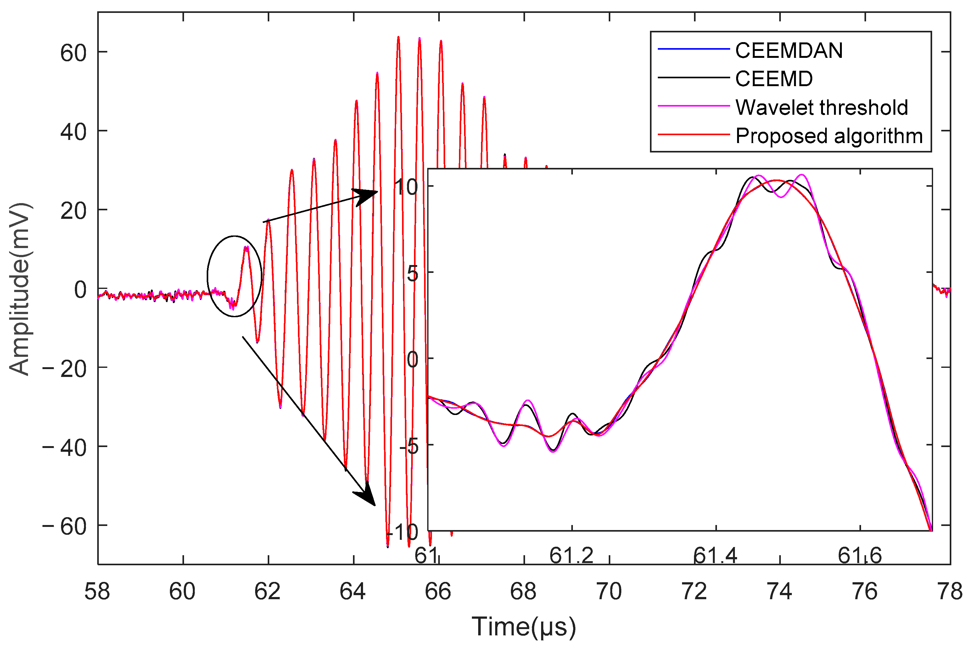
To illustrate the noise suppression effects of different methods, the 58 –78 range was highlighted, as presented in Figure 15. The proposed algorithm was compared to several traditional denoising methods, including CEEMD, CEEMDAN, and the wavelet thresholding algorithm. Our results demonstrate that the proposed algorithm achieved a smoother and more complete received signal at the receiving peak compared to the other three methods, which exhibited some noise in the parts before 60 and after 75 .
6. Conclusions
In this paper, an ultrasound echo signal denoising algorithm based on CEEMDAN, MIE, and improved wavelet thresholding is proposed. The method eliminates high-frequency components with excessive noise while maintaining the low-frequency characteristics that are dominated by the signal. This results in a reduction in noise levels, improving the quality and clarity of the echo signals while achieving effective signal denoising. First, the ultrasound echo signal with noise is decomposed using CEEMDAN. Then, it is divided into IMF components and residual signals, whose complexity is calculated using MIE. Next, the dominant part of the signal is extracted from the IMF components and wavelet-based thresholding is applied to denoise it. Finally, the denoised signal and residual signals are reconstructed. The denoising efficacy of the algorithm was confirmed using simulation experiments and an experimental oil level measurement device. In the future, the algorithm will be further refined to enhance its denoising effect and to improve its suitability for practical applications.
Author Contributions
Conceptualization, Z.L. and H.X.; methodology, Z.L. and H.X.; investigation, Z.L., H.X. and B.J.; validation, Z.L., H.X. and F.H.; data curation, Z.L., B.J. and F.H.; writing—original draft preparation, Z.L. and H.X.; writing—review and editing, Z.L., H.X., B.J. and F.H.; supervision, Z.L. and B.J.; project administration, Z.L. and F.H. All authors have read and agreed to the published version of the manuscript.
Funding
This research received no external funding.
Data Availability Statement
The data can be shared up on request.
Conflicts of Interest
The authors declare no conflict of interest.
Abbreviations
| EMD | Empirical Mode Decomposition |
| EEMD | Ensemble Empirical Mode Decomposition |
| CEEMD | Complementary Ensemble Empirical Mode Decomposition |
| CEEMDAN | Complete Ensemble Empirical Mode Decomposition with Adaptive Noise |
| IMF | Intrinsic Mode Function |
| NCC | Normalized Cross Correlation |
| RMSE | Root Mean Square Error |
| MIE | Mutual information entropy |
| VMD | Variational Mode Decomposition |
| GRA | Grey Relational Analysis |
| SSWT | Synchro Squeezing Wavelet Transform |
| WTD | Wavelet Threshold Denoising |
References
- Lu, Z.K.; Yang, C.; Qin, D.H.; Luo, Y.L.; Momayez, M. Estimating ultrasonic time-of-flight through echo signal envelope and modified Gauss Newton method. Measurement 2016, 94, 355–363. [Google Scholar] [CrossRef]
- Colantoni, A.; Cecchini, M.; Monarca, D.; Marcantonio, V. Ultrasonic waves for materials evaluation in fatigue, thermal and corrosion damage: A review. Mech. Syst. Signal Process. 2018, 120, 32–42. [Google Scholar]
- Ahila, A.; Poongodi, M.; Bourouis, S.; Band, S.S.; Mosavi, A.; Agrawal, S.; Hamdi, M. Meta-Heuristic Algorithm-Tuned Neural Network for Breast Cancer Diagnosis Using Ultrasound Images. Front. Oncol. 2022, 12, 834028. [Google Scholar]
- Al-Aufi, Y.A.; Hewakandamby, B.N.; Dimitrakis, G.; Holmes, M.; Watson, N.J. Thin film thickness measurements in two phase annular flows using ultrasonic pulse echo techniques. Flow Meas. Instrum. 2019, 66, 67–78. [Google Scholar] [CrossRef]
- Oral, M. Investigation of Surface Damages in Composite Materials Using Ultrasonic Lamb Waves. El-Cezeri 2021, 8, 652–665. [Google Scholar] [CrossRef]
- Stanišić, S.M.; Ignjatović, L.M.; Anðelković, I.; Stević, M.C.; Tasić, A.M.; Biserčić, M.S. Ultrasound-assisted extraction of matrix elements and heavy metal fractions associated with Fe, Al and Mn oxyhydroxides from soil. J. Serbian Chem. Soc. 2012, 77, 1287–1300. [Google Scholar] [CrossRef]
- Wang, B.; Zhong, S.; Lee, T.L.; Fancey, K.S.; Mi, J. Non-destructive testing and evaluation of composite materials/structures: A state-of-the-art review. Adv. Mech. Eng. 2020, 12, 152–169. [Google Scholar] [CrossRef] [Green Version]
- Wu, B.; Huang, Y.; Krishnaswamy, S. A Bayesian Approach for Sparse Flaw Detection from Noisy Signals for Ultrasonic NDT. NDT E Int. 2017, 85, 76–85. [Google Scholar] [CrossRef]
- Zhao, G.; Liu, S.; Zhang, C.; Jin, L.; Yang, Q. Ultrasonic nonlinear response of micro plastic damage on aluminum alloy plate with varying thickness. Jpn. J. Appl. Phys. 2022, 61, 016503. [Google Scholar] [CrossRef]
- Guo, R.; Chen, D.; Fei, C.; Li, D.; Zhang, Q.; Feng, W.; Yang, Y. Optimization design of high-frequency ultrasonic transducer based on ANFIS and particle swarm optimization algorithm. Appl. Acoust. 2022, 187, 108507. [Google Scholar] [CrossRef]
- Lu, Z.; Cui, Y.; Qin, D.; Luo, Y. Estimating the parameters of ultrasonic echo signal in the Gabor transform domain and its resolution analysis. Signal Process. 2016, 120, 607–619. [Google Scholar] [CrossRef]
- Wang, D.W.; Wang, Z.B.; Chen, Y.X.; Li, H.Y.; Wang, H.K. Ultrasonic echo processing method based on dual-Gaussian attenuation model. Acta Phys. Sin. 2019, 689, 084303055213. [Google Scholar] [CrossRef]
- Cheng, J.; Xu, Y.; Ding, D.; Liu, W. A novel de-noising method based on coherence average for ultrasonic signal of partial discharge in transformer. IET Sci. Meas. Technol. 2021, 15, 302–311. [Google Scholar] [CrossRef]
- Cooper, J.; Tran, A.N.; Wallander, S. Testing for Specification Bias with a Flexible Fourier Transform Model for Crop Yields. Am. J. Agric. Econ. 2017, 99, 800–817. [Google Scholar] [CrossRef] [Green Version]
- Rhif, M.; Abbes, A.B.; Farah, I.; Martínez, B.; Sang, Y. Wavelet Transform Application for/in Non-Stationary Time-Series Analysis: A Review. Appl. Sci. 2019, 9, 1345. [Google Scholar] [CrossRef] [Green Version]
- Imaouchen, Y.; Kedadouche, M.; Alkama, R.; Thomas, M. A Frequency-Weighted Energy Operator and complementary ensemble empirical mode decomposition for bearing fault detection. Mech. Syst. Signal Process. 2017, 82, 103–116. [Google Scholar] [CrossRef]
- Gu, J.; Peng, Y.X. An improved complementary ensemble empirical mode decomposition method and its application in rolling bearing fault diagnosis. Digit. Signal Process. 2021, 113, 103050. [Google Scholar] [CrossRef]
- Liu, Y.; Ma, K.; He, H.; Gao, K. Obtaining Information about Operation of Centrifugal Compressor from Pressure by Combining EEMD and IMFE. Entropy 2020, 22, 424. [Google Scholar] [CrossRef] [Green Version]
- Ke, Z.; Di, C.; Bao, X. Adaptive Suppression of Mode Mixing in CEEMD Based on Genetic Algorithm for Motor Bearing Fault Diagnosis. IEEE Trans. Magn. 2021, 58, 8200706. [Google Scholar] [CrossRef]
- Torres, M.E.; Colominas, M.A.; Schlotthauer, G.; Flandrin, P. A complete ensemble empirical mode decomposition with adaptive noise. In Proceedings of the 2011 IEEE International Conference on Acoustics, Speech and Signal Processing (ICASSP), Prague, Czech Republic, 22–27 May 2011; pp. 4144–4147. [Google Scholar] [CrossRef]
- Li, T.; Qian, Z.; He, T. Short-Term Load Forecasting with Improved CEEMDAN and GWO-Based Multiple Kernel ELM. Complexity 2020, 2020, 1209547. [Google Scholar] [CrossRef] [Green Version]
- Sabatini, A.M. Correlation receivers using Laguerre filter banks for modelling narrowband ultrasonic echoes and estimating their time-of-flights. IEEE Trans. Ultrason. Ferroelectr. Freq. Control 2002, 44, 1253–1263. [Google Scholar] [CrossRef]
- Demirli, R.; Saniie, J. Model-based estimation of ultrasonic echoes. Anal. Algorithms. IEEE Trans. Ultrason. Ferroelectr. Freq. Control 2001, 48, 787. [Google Scholar] [CrossRef]
- Huang, N.E.; Shen, Z.; Long, S.R.; Wu, M.C.; Shih, H.H.; Zheng, W.; Yen, N.; Tung, C.C.; Liu, H.H.; Yen, N.C. The empirical mode decomposition method and the Hilbert spectrum for non-stationary time series analysis. Proc. R. Soc. Lond. Ser. A Math. Phys. Eng. Sci. 1998, 454, 903–995. [Google Scholar] [CrossRef]
- Wu, Z.; Huang, N.E. Ensemble Empirical Mode Decomposition: A Noise-Assisted Data Analysis Method. Adv. Adapt. Data Anal. 2011, 1, 1–41. [Google Scholar] [CrossRef]
- Lei, Y.; Liu, Z.; Ouazri, J.; Lin, J. A fault diagnosis method of rolling element bearings based on CEEMDAN. Proc. Inst. Mech. Eng. C J. Mech. Eng. Sci. 2017, 231, 1804–1815. [Google Scholar] [CrossRef]
- Olvera-Guerrero, O.A.; Prieto-Guerrero, A.; Espinosa-Paredes, G. Decay Ratio estimation in BWRs based on the improved complete ensemble empirical mode decomposition with adaptive noise. Ann. Nucl. Energy 2017, 102, 280–296. [Google Scholar] [CrossRef]
- Shuang, G.; Xiao-Li, L.; Fei, L. Near Infrared Spectroscopy Process Pattern Fault Detection Based on Mutual Information Entropy. Spectrosc. Spectr. Anal. 2019, 39, 1736–1741. [Google Scholar]
- Omitaomu, O.A.; Protopopescu, V.A.; Ganguly, A.R. Empirical Mode Decomposition Technique with Conditional Mutual Information for Denoising Operational Sensor Data. IEEE Sens. J. 2011, 11, 2565–2575. [Google Scholar] [CrossRef]
- Lei, Z.; Su, W.; Hu, Q. Multimode Decomposition and Wavelet Threshold Denoising of Mold Level Based on Mutual Information Entropy. Entropy 2019, 21, 202. [Google Scholar] [CrossRef] [Green Version]
- Donoho, D.L.; Johnstone, J.M. Ideal spatial adaptation by wavelet shrinkage. Biometrika 1994, 81, 425–455. [Google Scholar] [CrossRef]
- Peng, T.; Bao-Ping, G. Wavelet Denoising Based on Modified Threshold Function Optimization Method. J. Signal Process. 2017, 8, 1259–1284. [Google Scholar]
- Jiao, Y.; Li, Z.; Zhu, J.; Xue, B.; Zhang, B. ABIDE: A Novel Scheme for Ultrasonic Echo Estimation by Combining CEEMD-SSWT Method with EM Algorithm. Sustainability 2022, 14, 1960. [Google Scholar] [CrossRef]
Figure 1.
Gaussian model for ultrasonic signals.

Figure 2.
Results of CEEMDAN decomposition.

Figure 3.
Wavelet threshold denoising flowchart.

Figure 4.
Curve comparison between the improved threshold function and the hard/soft threshold functions.
Figure 4.
Curve comparison between the improved threshold function and the hard/soft threshold functions.

Figure 5.
Process diagram of the proposed wavelet threshold function denoising system based on CEEMDAN.
Figure 5.
Process diagram of the proposed wavelet threshold function denoising system based on CEEMDAN.

Figure 6.
Time-domain plot of ultrasonic echoes. (a) Pure ultrasonic echo signal. (b) Ultrasonic echo signal with a signal-to-noise ratio of 9dB.
Figure 6.
Time-domain plot of ultrasonic echoes. (a) Pure ultrasonic echo signal. (b) Ultrasonic echo signal with a signal-to-noise ratio of 9dB.

Figure 7.
CEEMDAN decomposition of a noisy signal with an SNR of 9 dB.

Figure 8.
Signal’s dominant portion identified through MIE filtering.

Figure 9.
Comparison between the original noisy signal and the received signal.

Figure 10.
Schematic diagram of an engine oil level detection experiment.

Figure 11.
Time-domain curve of actual signal received by the transducer.

Figure 12.
CEEMDAN decomposition of the ultrasonic echo signal in the oil medium.

Figure 13.
Filtered signal-dominant section.

Figure 14.
Comparison of signal received by the transducer to the curve obtained after applying the proposed denoising algorithm.
Figure 14.
Comparison of signal received by the transducer to the curve obtained after applying the proposed denoising algorithm.

Figure 15.
Effectiveness comparison chart of different noise reduction algorithms on received signals.
Figure 15.
Effectiveness comparison chart of different noise reduction algorithms on received signals.


Table 1.
MIE values of adjacent IMFs.
| IMF1–2 | IMF2–3 | IMF3–4 | IMF4–5 | IMF5–6 | IMF6–7 | IMF7–8 | IMF8–9 | IMF9–R |
|---|---|---|---|---|---|---|---|---|
| 1.945 | 2.053 | 2.502 | 1.338 | 1.706 | 2.215 | 2.791 | 3.612 | 4.252 |
Table 2.
Different indicators of the original noisy signal after denoising with the proposed algorithm.
Table 2.
Different indicators of the original noisy signal after denoising with the proposed algorithm.
| SNR of the Noisy Signal (dB) | Received Signal | ||
|---|---|---|---|
| SNR (dB) | RMSE | NCC | |
| 0 | 12.6890 | 0.0580 | 0.97412 |
| 3 | 15.2926 | 0.0430 | 0.98552 |
| 6 | 18.9602 | 0.0282 | 0.99373 |
| 9 | 21.8262 | 0.0202 | 0.99675 |
| 12 | 24.6710 | 0.0146 | 0.99830 |
| 15 | 27.5058 | 0.0105 | 0.99911 |
| 18 | 29.9366 | 0.0079 | 0.99950 |
| 21 | 32.2653 | 0.0061 | 0.99971 |
| 24 | 34.4046 | 0.0048 | 0.99982 |
| 27 | 36.5031 | 0.0037 | 0.99989 |
| 30 | 37.4580 | 0.0034 | 0.99992 |
Table 3.
Comparison of noise reduction outcomes obtained using different denoising algorithms.
| Denoising Algorithm | SNR (dB) | RMSE | NCC |
|---|---|---|---|
| CEEMD | 16.3761 | 0.0379 | 0.98845 |
| CEEMDAN | 19.9904 | 0.0250 | 0.99500 |
| Wavelet Threshold | 20.1588 | 0.0245 | 0.99527 |
| Proposed Algorithm | 21.8262 | 0.0202 | 0.99675 |
Table 4.
Comparison of several advanced echo signal processing methods.
| Group | Research Methodology | SNR (dB) | RMSE | References |
|---|---|---|---|---|
| A | VMD-MIE-WTD | 20.494 | 0.021 | [30] |
| B | CEEMD-GRA-SSWT | 20.936 | 0.020 | [33] |
| C | Proposed Algorithm | 21.062 | 0.019 | * |
* denotes the algorithm in this paper.
Table 5.
MIE values of adjacent IMFs.
| (a) | |||||||||
|---|---|---|---|---|---|---|---|---|---|
| IMF1–2 | IMF2–3 | IMF3–4 | IMF4–5 | IMF5–6 | IMF6–7 | IMF7–8 | IMF8–9 | IMF9–10 | |
| 2.729 | 2.688 | 2.630 | 2.490 | 2.372 | 2.579 | 2.778 | 0.987 | 1.529 | |
| (b) | |||||||||
| IMF10–11 | IMF11–12 | IMF12–13 | IMF13–14 | IMF14–15 | IMF15–16 | IMF16–17 | IMF17–R | ||
| 2.120 | 2.531 | 3.135 | 4.540 | 5.775 | 6.364 | 7.000 | 7.586 | ||
Disclaimer/Publisher’s Note: The statements, opinions and data contained in all publications are solely those of the individual author(s) and contributor(s) and not of MDPI and/or the editor(s). MDPI and/or the editor(s) disclaim responsibility for any injury to people or property resulting from any ideas, methods, instructions or products referred to in the content. |
© 2023 by the authors. Licensee MDPI, Basel, Switzerland. This article is an open access article distributed under the terms and conditions of the Creative Commons Attribution (CC BY) license (https://creativecommons.org/licenses/by/4.0/).
Share and Cite
MDPI and ACS Style
Li, Z.; Xu, H.; Jiang, B.; Han, F. Wavelet Threshold Ultrasound Echo Signal Denoising Algorithm Based on CEEMDAN. Electronics 2023, 12, 3026. https://doi.org/10.3390/electronics12143026
AMA Style
Li Z, Xu H, Jiang B, Han F. Wavelet Threshold Ultrasound Echo Signal Denoising Algorithm Based on CEEMDAN. Electronics. 2023; 12(14):3026. https://doi.org/10.3390/electronics12143026
Chicago/Turabian StyleLi, Zhiwei, Huyue Xu, Bibo Jiang, and Fangfang Han. 2023. "Wavelet Threshold Ultrasound Echo Signal Denoising Algorithm Based on CEEMDAN" Electronics 12, no. 14: 3026. https://doi.org/10.3390/electronics12143026
Note that from the first issue of 2016, this journal uses article numbers instead of page numbers. See further details here.