Cost-Sensitive Broad Learning System for Imbalanced Classification and Its Medical Application

Abstract

As an effective and efficient discriminative learning method, the broad learning system (BLS) has received increasing attention due to its outstanding performance without large computational resources. The standard BLS is derived under the minimum mean square error (MMSE) criterion, while MMSE is with poor performance when dealing with imbalanced data. However, imbalanced data are widely encountered in real-world applications. To address this issue, a novel cost-sensitive BLS algorithm (CS-BLS) is proposed. In the CS-BLS, many variations can be adopted, and CS-BLS with weighted cross-entropy is analyzed in this paper. Weighted penalty factors are used in CS-BLS to constrain the contribution of each sample in different classes. The samples in minor classes are allocated higher weights to increase their contributions. Four different weight calculation methods are adopted to the CS-BLS, and thus, four CS-BLS methods are proposed: Log-CS-BLS, Lin-CS-BLS, Sqr-CS-BLS, and EN-CS-BLS. Experiments based on artificially imbalanced datasets of MNIST and small NORB are firstly conducted and compared with the standard BLS. The results show that the proposed CS-BLS methods have better generalization and robustness than the standard BLS. Then, experiments on a real ultrasound breast image dataset are conducted, and the results demonstrate that the proposed CS-BLS methods are effective in actual medical diagnosis.

1. Introduction

The broad learning system (BLS) is an efficient and effective machine learning technique, which is designed by the inspiration of the random vector functional-link neural network (RVFLNN) [1,2]. As the pseudo-inverse algorithm is used to compute the output weights of the standard BLS, the BLS has the characteristic of an efficient operation speed, and thus, it is adopted in many real-world applications, such as medical data analysis [3], fault diagnosis [4], and robotics [5]. In addition, many varieties based on BLS are developed to adapt it to target application domains. A sparse Bayesian BLS was proposed in [6] for probabilistic estimation. A gradient descent-based BLS was proposed in [7] for the control of nonlinear dynamic systems, which adopted gradient descent other than the pseudo-inverse algorithm to calculate the weight matrix in BLS iteratively.

The imbalanced classification problem that suffers from imbalanced class distributions is encountered in many real-world domains, such as medical diagnosis [8], abnormal activity recognition [9], fault diagnosis [10], and fraud detection [11]. The difficulty with class imbalance learning is that the common classification methods probably predict samples in minority classes as rare occurrences, even as outliers or noise, which causes samples in minority classes to be misclassified. Generally, minority classes are of greater importance and deserve more attention. Taking breast cancer diagnosis as an example [12], detecting the minority class (i.e., the class of malignant lesions) should draw more attention, and the accurate diagnosis of it at early stages would increase the survival rate of patients. However, as the benign samples are far more than the malignant samples, the collected dataset would make the learned diagnostic strategy with a large deviation.

On a broader level, researchers in different communities, such as machine learning and medical diagnosis, devote great efforts to it to handle the imbalanced classification problem, and various methods were proposed during the last decades [13,14]. Generally, the methods can be grouped as data-level methods, classifier-level methods, and hybrid methods.

Data-level methods alter the distribution of the training set by artificially adding or subtracting samples to provide a balanced distribution [15]. The key idea of these methods is the mechanism used for sampling the original training set. The sampling mechanisms in this area can be roughly categorized into over-sampling methods, under-sampling methods, and dynamic sampling methods [15]. Over-sampling methods randomly duplicate the samples of the minority classes to increase their contributions, such as random over-sampling [16], synthetic minority over-sampling technique (SMOTE) [17], and ranked minority over-sampling in boosting (RAMOBoost) [18]. Particularly, many variants of SMOTE were developed based on different sample weight calculation methods, such as the adaptive synthetic sampling approach (ADASYN) [19], borderline-SMOTE [20], and majority weighted SMOTE (MWMOTE) [21]. ADASYN adopted a density distribution as its criterion to generate samples for different minority classes. Borderline-SMOTE only paid attention to minority cases around the class boundary. MWMOTE first discovered the difficult-to-learn minority class examples and then assigned them substantial weights based on their Euclidean distance from the adjacent majority class samples. Under-sampling methods randomly select a percentage of data from the majority classes, including clustering-based under-sampling [22], decontamination-based under-sampling [23], etc. The dynamic sampling methods over-sample the minority classes and under-sample the majority classes, which is a combination of the above two sampling methods, such as dynamic sampling networks (DSN) [24] and context-guided dynamic sampling (CGDS) [25].

Classifier-level methods modify the used classifier directly or design a new classifier to deal with imbalanced classification problems. One kind of method in this area is called cost-sensitive methods, which design different misclassification costs for different samples, such as weighted extreme learning machine (WELM) [26], the cost-sensitive decision tree ensemble method [27], cost-sensitive cross-entropy for multilayer perceptron neural networks (CSEFMLP) [28], and cost-sensitive deep neural networks (CSDNN) [29]. WELM [26] penalizes misclassified minority class samples more severely with a larger penalty than misclassified majority class samples. The cost-sensitive decision tree ensemble method proposed in [27] combines cost-sensitive decision trees with random subspace-based feature space partitioning to boost the recognition rate of the minority class. CSEFMLP [28] adopts the prior probabilities ratio of the target classes to compensate the class imbalance and thus incorporate the prior probability ratio into the cross-entropy (CE) loss. CSDNN [29] adopts a cost-sensitive stacked denoising autoencoder to conduct real-life applications. Another kind of classifier-level method increases the importance of the minority class by changing the objective function of the classifier. Wang et al. [30] developed two new loss functions, mean false error (MFE) and mean squared false error (MSFE), that are more sensitive to the errors from the minority class. The MSFE loss improves on the MFE loss, and it can better capture errors from the positive class. Lin et al. [31] proposed the focal loss (FL) to battle severe imbalances by reshaping the CE loss to decrease the influence of easily classified data on the loss.

Hybrid methods combine multiple techniques from classifier-level methods and data-level methods. One of the most well-known methods in this group is called ensemble learning. Liu et al. [32] proposed EasyEnsemble and BalanceCascade to train a series of classifiers on under-sampled subsets. SMOTEBoost, on the other hand, combines boosting with SMOTE over-sampling [33]. A two-phase learning approach was proposed for brain tumor segmentation, and the results showed its success [34]. The novel research field successfully combines machine learning and swarm intelligence approaches and proved to be able to obtain outstanding results in different areas [35,36].

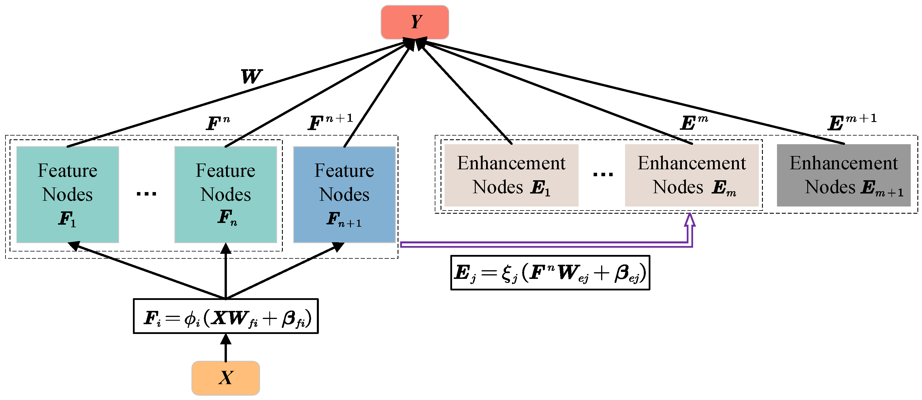
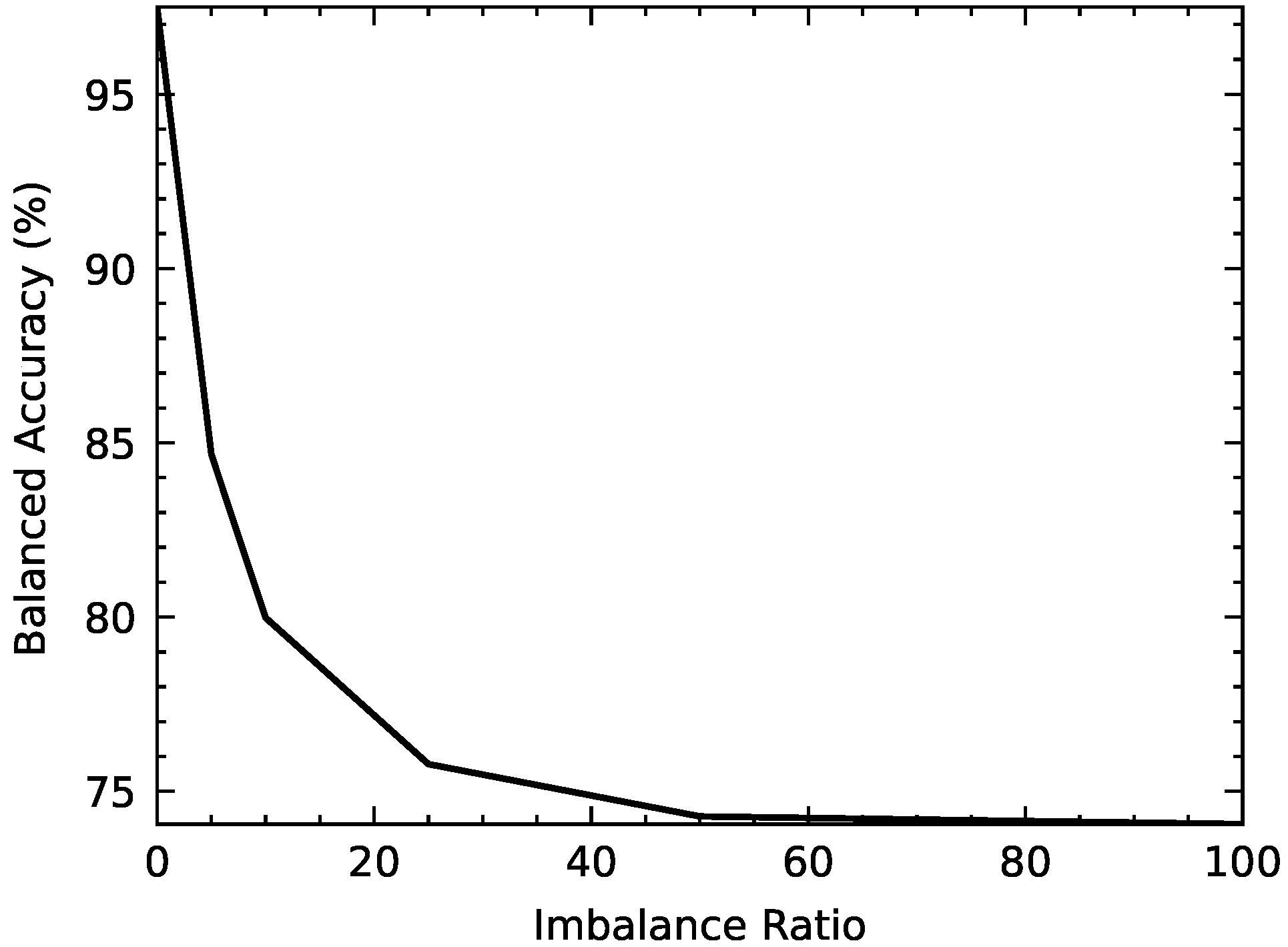
The structure of BLS is shown in Figure 1. The standard BLS first processes input data ($\mathit{X}$) with randomly initialized weights (${\mathit{W}}_{fi}$ and ${\mathit{\beta }}_{fi}$) and a series of activation functions (${\varphi }_i$) as its feature nodes, and then, feature nodes are mapped to enhancement nodes with random weights (${\mathit{W}}_{ej}$ and ${\mathit{\beta }}_{ej}$) and a series of nonlinear activation functions (${\xi }_j$). After that, the pseudoinverse of all nodes with actual ouputs $\mathit{Y}$ by the ridge regression approximation is conducted to calculate the weight matrix $\mathit{W}$, which can refer to [1]. When BLS is used to deal with imbalanced classification problems, the standard BLS is with poor performance when dealing with imbalanced data. The reason is that the weight matrix $\mathit{W}$ is calculated based on the ridge regression approximation, while the ridge regression approximation is derived under the minimum mean square error (MMSE) criterion. Taking a common dataset, MNIST [37], as an example, the balanced accuracy of BLS decreases steeply as the imbalance ratio of MNIST increases, as shown in Figure 2.

To our best knowledge, only several related methods on BLS were developed to handle this problem. A cost-sensitive rich feature combination BLS (cost-sensitive R-BLS) was proposed in [38] for imbalanced classification. Another cost-sensitive method on BLS includes weighted BLS (W-BLS) [39], evolutionary-based W-BLS (EW-BLS) [40], and weighted generalized cross-validation-based regularized BLS (WGCV-BLS) [41]. A hybrid approach based on BLS, incremental weighted ensemble BLS (IWEBLS) [42], was developed for imbalanced classification. The above cost-sensitive methods are based on the weighted mean square error loss function. The maximum correntropy criterion was adopted in [43] as the loss function of BLS to handle imbalanced data, and the corresponding results showed its success on different application domains. However, there is no common framework that can effectively integrate different cost-sensitive loss functions easily to improve the performance of BLS in handling imbalanced data.

Class imbalance is an urgent problem that needs to be handled in object detection, and weighted cross-entropy (WCE) is one of the most effective techniques in this area [44]. Inspired by this and the above analysis [7,28,43], WCE is adopted to analyze the imbalance classification problems of the CS-BLS framework. In this paper, an improved BLS for imbalanced classification problems is proposed for handling imbalanced classification problems. This BLS algorithm adopts cost-sensitive loss functions, such as WCE, rather than the standard MMSE. In addition, four CS-BLS methods are proposed, which adopted four different methods for calculating the weighted penalty factors to constrain the contribution of each sample in different classes. Several commonly used datasets are adopted to evaluate the effectiveness of the proposed methods in different imbalanced ratios and broad structures and their performance on medical applications. The main contributions of this work can be summarized into three aspects:

• A cost-sensitive BLS framework, CS-BLS, is proposed to improve the performance of standard BLS on imbalanced classification problems;
• Four CS-BLS approaches are proposed, and each approach adopts a different penalty factor calculation method based on inverse class frequency or effective numbers;
• A systemic experimental study on the CS-BLS is conducted, in which two commonly used datasets with different imbalanced ratios and a clinical ultrasound image diagnosis dataset are utilized.

The remainder of this paper is organized as follows. Section 2 elaborates the proposed CS-BLS and its varieties based on different calculation methods of the weighted penalty factors. In Section 3, a list of experiments is first presented based on two commonly used datasets to demonstrate the effectiveness and robustness of the CS-BLS. Then, a clinical ultrasound image diagnosis dataset is adopted to evaluate the performance of CS-BLS on medical diagnosis. At last, a conclusion is given in Section 5.

2. Proposed Method

2.1. Cost-Sensitive Broad Learning System (CS-BLS)

Unlike the standard BLS [1], the proposed CS-BLS adopts a cost-sensitive loss function as its loss function to improve the ability of BLS when handling imbalanced classification problems. In the imbalanced training dataset $\left\{\mathit{X},\mathit{Y}\right\}$ ($\mathit{X}\in {\mathbb{R}}^{N\times D}$, $\mathit{Y}\in {\mathbb{R}}^{N\times l}$), the letters N, D, and l represent the number of samples in the input dataset, the dimension of input data and the dimension of outputs, respectively. The details are listed as follows.

Firstly, similar to BLS [1], all training data $\mathit{X}$ are projected to the ith set of feature nodes ${\mathit{F}}_i$ using a linear activation function.

$${\mathit{F}}_i={\varphi }_i\left(\mathit{X}{\mathit{W}}_{fi}+{\mathit{\beta }}_{fi}\right),$$

(1)

where ${\mathit{W}}_{fi}$ and ${\mathit{\beta }}_{fi}$ are randomly generated weights with proper dimensions. Each map has k feature nodes, and k is a hyper parameter. ${\varphi }_i\left(·\right)$ indicates the ith linear activation function. After that, feature nodes in each map are concatenated as ${\mathit{F}}^n$,

$${\mathit{F}}^n\equiv \left[{\mathit{F}}_1,\dots ,{\mathit{F}}_n\right],$$

(2)

where n is the number of feature node maps. ${\mathit{F}}^n\in {\mathbb{R}}^{\left(N\times nk\right)}$ and N is the number of samples in $\mathit{X}$.

Then, ${\mathit{F}}^n$ is subjected to a nonlinear activation function ${\xi }_j$ to produce the jth set of enhancement node map ${\mathit{E}}_j$,

$${\mathit{E}}_j={\xi }_j\left({\mathit{F}}^n{\mathit{W}}_{ej}+{\mathit{\beta }}_{ej}\right),$$

(3)

where ${\mathit{W}}_{ej}$ and ${\mathit{\beta }}_{ej}$ are randomly generated weights with proper dimensions, and ${\xi }_j\left(·\right)$ is a nonlinear activation function. Each map has q enhancement nodes, and q is a hyper parameter. Then, enhancement nodes in all maps are concatenated as $E^m$,

$${\mathit{E}}^m\equiv \left[{\mathit{E}}_1,\dots ,{\mathit{E}}_m\right],$$

(4)

where m is the number of enhancement node maps and ${\mathit{E}}^m\in {\mathbb{R}}^{\left(N\times mq\right)}$.

Then, the enhancement nodes ${\mathit{E}}^m$ and feature nodes ${\mathit{F}}^n$ are concatenated as ${\mathit{S}}_m^n$,

$${\mathit{S}}_m^n=\left[{\mathit{F}}^n\mid {\mathit{E}}^m\right],$$

(5)

where ${\mathit{S}}_m^n\in {\mathbb{R}}^{N\times \left(nk+mq\right)}$.

Afterwards, the outputs of the broad learning system under enhancement nodes ${\mathit{E}}^m$ and feature nodes ${\mathit{F}}^n$ are $\mathit{Z}$,

$$\mathit{Z}={\mathit{S}}_m^n{\mathit{W}}_m^n,$$

(6)

where ${\mathit{W}}_m^n$ is the required weights in the BL structure.

Taking WCE loss function as an example, a softmax layer is utilized after the outputs $\mathit{Z}$ when calculating WCE loss. Supposing $z_r\in \mathit{Z}\left(r=1,2,\dots ,N\right)$ and $z_r={\left[z_r^1,z_r^2,\dots ,z_r^C\right]}^{\top }$, the corresponding true label is ${\mathbf{y}}_r$ (${\mathbf{y}}_r\in \mathit{Y}$) and ${\mathbf{y}}_r$ is a one-hot C-element vector indicating the ground-truth label and ${\mathbf{y}}_r={\left[y_r^1,y_r^2,\dots ,y_r^C\right]}^{\top }$, in which we suppose $y_r^c=1$ ($c=1,2,\dots ,C$). The softmax function regards each class as mutually exclusive and calculates the probability distribution over all classes as $p_i=\exp \left(z_i\right)/{\displaystyle {\sum }_{j=1}^C}\exp \left(z_j\right),\forall i\in \left\{1,2,\dots ,C\right\}$. Therefore, supposing the weight of class c is ${\omega }_c$, the loss function of the proposed CS-BLS can be written as,

$$L=-\frac{1}{N}{\displaystyle \sum _{r=1}^N}{\displaystyle \sum _{c=1}^C}{\omega }_c{y}_r^c\log \left(\frac{\exp \left(z_r^c\right)}{{\displaystyle {\sum }_{j=1}^C}\exp \left(z_r^j\right)}\right),$$

(7)

where $y_r^c$ is an indicator variable, which indicates when it is true, $y_r^c=1$, else $y_r^c=0$. ${\omega }_c$ is a weight in the weight vector $\mathit{\omega }={[{\omega }_1,{\omega }_2,\dots ,{\omega }_C]}^T$, in which the value can be user-chosen class by class and fixed or automatically adjusted during the training process of the CS-BLS. In the CS-BLS framework, the gradient decent method is adopted to obtain trained ${\mathit{W}}_m^n$, other than the ridge regression method in standard BLS. The methods of calculating weighted penalty factors can be referred to in Section 2.2.

Suppose the above update processes cannot achieve the desired performance. In that case, a feature map may be added to the original broad structure. The added features nodes ${\mathit{F}}_{n+1}$ and the related enhancement nodes ${\mathit{E}}_{e{x}_m}$ are produced randomly as follows,

$${\mathit{F}}_{n+1}={\varphi }_{n+1}\left(\mathit{X}{\mathit{W}}_{e_{n+1}}+{\mathit{\beta }}_{e_{n+1}}\right),$$

(8)

$${\mathit{E}}_{e{x}_m}=\left[{\xi }_1\left({\mathit{F}}_{n+1}{\mathit{W}}_{e{x}_1}+{\mathit{\beta }}_{e{x}_1}\right),\dots ,{\xi }_m\left({\mathit{F}}_{n+1}{\mathit{W}}_{e{x}_m}+{\mathit{\beta }}_{e{x}_m}\right)\right],$$

(9)

where ${\mathit{W}}_{e_{n+1}}$, ${\mathit{W}}_{e{x}_j}$, ${\mathit{\beta }}_{e_{n+1}}$, and ${\mathit{\beta }}_{e{x}_j}$ ($j=1,2,\dots ,m$) are randomly generated, and ${\varphi }_{n+1}\left(·\right)$ is the $(n+1)$th linear activation function. By defining ${\mathit{S}}_m^{n+1}\equiv \left[{\mathit{S}}_m^n\mid {\mathit{F}}_{n+1}^{}\mid {\mathit{E}}_{e{x}_m}\right]$, ${\left({\mathit{S}}_m^{n+1}\right)}^{+}$ is upgraded as follows [1],

$${\left({\mathit{S}}_m^{n+1}\right)}^{+}=\left[\begin{array}{c}{\left({\mathit{S}}_m^n\right)}^{+}-\mathit{C}{\mathit{B}}^T\\ {\mathit{B}}^T\end{array}\right],$$

(10)

where $\mathit{C}={\left({\mathit{S}}_m^n\right)}^{+}\left[{\mathit{F}}_{n+1}^{}\mid {\mathit{E}}_{e{x}_m}\right]$, ${\mathit{B}}^T=\left\{\begin{array}{cc}{\left(\mathit{D}\right)}^{+}& \mathrm{if}\mathit{D}\ne 0\\ {\left(\mathbf{1}+{\mathit{C}}^T\mathit{C}\right)}^{-1}{\mathit{C}}^T{\left({\mathit{S}}_m^n\right)}^{+}& \mathrm{if}\mathit{D}=0\end{array}\right.$ and $\mathit{D}=\left[{\mathit{F}}_{n+1}\mid {\mathit{E}}_{e{x}_m}\right]-{\mathit{S}}_m^n\mathit{C}$.

An enhancement map may also be added to the original broad structure for the same purpose. The added enhancement nodes are produced randomly as follows,

$${\mathit{E}}_{m+1}={\xi }_{m+1}\left({\mathit{F}}^n{\mathit{W}}_{h_{m+1}}+{\mathit{\beta }}_{h_{m+1}}\right),$$

(11)

where ${\mathit{W}}_{h_{m+1}}$, ${\mathit{\beta }}_{h_{m+1}}$ are randomly produced, and ${\xi }_{m+1}\left(·\right)$ is the $(m+1)$th nonlinear activation function. Concatenating the previous nodes ${\mathit{S}}_m^n$ with ${\mathit{E}}_{m+1}$, ${\mathit{S}}_{m+1}^n$ is obtained by horizontal concatenation, which is shown as follows,

$${\mathit{S}}_{m+1}^n\equiv \left[{\mathit{S}}_m^n\mid {\mathit{E}}_{m+1}^{}\right].$$

(12)

Hence, according to the Moore–Penrose inverse theory for a partitioned matrix [1], ${\left({\mathit{S}}_{m+1}^n\right)}^{+}$ is derived as follows,

$${\left({\mathit{S}}_{m+1}^n\right)}^{+}=\left[\begin{array}{c}{\left({\mathit{S}}_m^n\right)}^{+}-{\mathit{C}}^{\prime }{{\mathit{B}}^{\prime }}^T\\ {{\mathit{B}}^{\prime }}^T\end{array}\right],$$

(13)

where ${\mathit{C}}^{\prime }={\left({\mathit{S}}_m^n\right)}^{+}{\mathit{E}}_{m+1}$, ${{\mathit{B}}^{\prime }}^T=\left\{\begin{array}{cc}{\left({\mathit{D}}^{\prime }\right)}^{+}& \mathrm{if}{\mathit{D}}^{\prime }\ne 0\\ {\left(1+{{\mathit{C}}^{\prime }}^T{\mathit{C}}^{\prime }\right)}^{-1}{{\mathit{C}}^{\prime }}^T{\left({\mathit{S}}_m^n\right)}^{+}& \mathrm{if}{\mathit{D}}^{\prime }=0\end{array}\right.$ and ${\mathit{D}}^{\prime }=$

$\left({\mathit{E}}_{m+1}-{\mathit{S}}_m^n{\mathit{C}}^{\prime }\right)$.

2.2. Methods for Calculating Weighted Penalty Factors

This section introduces four methods for calculating weighted penalty factors based on inverse class frequency and effective numbers.

2.2.1. Calculation Methods Based on Inverse Class Frequency

Class frequency allows the classifier to use information from different classes. It is regarded as an inter-class factor. To reflect the important level of each class, inverse class frequency is a good solution to it. There are three common methods of inverse class frequency, which are logarithmic inverse class frequency, linear inverse class frequency, and square root inverse class frequency [45]. In this paper, the above three kinds of methods of inverse class frequency are adopted to calculate the weighted penalty vector $\omega$, which are defined as follows,

$${\mathit{\omega }}^{Log}={\left[\ln \frac{N}{N_1},\ln \frac{N}{N_2},\dots ,\ln \frac{N}{N_C}\right]}^{\mathrm{T}},$$

(14)

$${\mathit{\omega }}^{Lin}={\left[\frac{N}{N_1},\frac{N}{N_2},\dots ,\frac{N}{N_C}\right]}^{\mathrm{T}},$$

(15)

$${\mathit{\omega }}^{Sqr}={\left[\sqrt{\frac{N}{N_1}},\sqrt{\frac{N}{N_2}},\dots ,\sqrt{\frac{N}{N_C}}\right]}^{\mathrm{T}},$$

(16)

where ${\mathit{\omega }}^{Log}$, ${\mathit{\omega }}^{Lin}$, and ${\mathit{\omega }}^{Sqr}$ are the logarithmic weighted penalty vector, linear weighted penalty vector, and square root weighted penalty vector, respectively. N is the total number of samples in the imbalanced training set. $N_c$ is the number of classes c ($c=1,2,\dots ,C$) in the imbalanced training set. Thus, the CS-BLS based on ${\mathit{\omega }}^{Log}$, ${\mathit{\omega }}^{Lin}$, and ${\mathit{\omega }}^{Sqr}$ are called Log-CS-BLS, Lin-CS-BLS, and Sqr-CS-BLS, respectively.

2.2.2. Calculation Methods Based on Effective Numbers

An effective weighted penalty factor calculation method was proposed in [46], which re-balanced the classification loss using the effective number of samples for each class. The volume of samples defines the effective number of class c, which can be computed as,

$${\epsilon }_c=\frac{1-{\beta }^{N_c}}{1-\beta },$$

(17)

where ${\epsilon }_c$ is the effective number of class c, and $\beta \in [0,1)$ is a hyper-parameter. Thus, the effective number based weighted penalty vector ${\mathit{\omega }}^{EN}$ is obtained as follows,

$${\mathit{\omega }}^{EN}={\left[\frac{1}{{\epsilon }_1},\frac{1}{{\epsilon }_2},\dots ,\frac{1}{{\epsilon }_C}\right]}^{\mathrm{T}}.$$

(18)

Thus, the CS-BLS based on calculation methods of ${\mathit{\omega }}^{EN}$ is called EN-CS-BLS.

3. Experiments and Results

Experiments are conducted to evaluate the effectiveness of the proposed CS-BLS methods based on three widely used datasets. To verify the robustness and generalization of four CS-BLS methods on different imbalance ratios, the MNIST dataset and small NORB dataset are artificially reconstructed to different imbalance ratios. Since the broad structure is significant to the performance of the BLS, a series of experiments are conducted on different broad structures to verify the performance of the CS-BLS methods and the standard BLS. A clinical breast ultrasound dataset is adopted to evaluate the performance of CS-BLS methods on medical applications. We performed all experiments on Legion R7000 2020, equipped with GPU NVIDIA 1660Ti, CPU AMD Ryzen 5 4600H @3.0 GHz, and 32G RAM. The PyTorch framework was adopted to build models, and all methods were implemented in Python.

3.1. Evaluation Metrics

The metrics used in imbalanced classification problems are quite different from those used in standard classification problems. In this paper, six widely used evaluation metrics in imbalanced classification problems are utilized, which are Balanced Accuracy (B_ACC), Recall, Precision, Area Under the Receiver Operating Characteristics Curve (AUC), F${}_1$-score, and Matthews correlation coefficient (MCC). It calculates the average percentage of positive and negative class instances that are correctly classified. Recall, also known as True Positive Rate or Sensitivity, is the percentage of the positive group that the classifier properly classifies as positive. Precision is the proportion of positively classified samples that are actually positive. AUC is a summary metric form of the Receiver Characteristics Curve (ROC), and it can be used to compare the performance between models. F${}_1$-score attempts to measure the trade-off between Precision and Recall by generating a single value that reflects the effectiveness of a classifier in the presence of rare classes. The MCC is a coefficient of correlation between observed and predicted classes. It ranges from −1 to +1. When the MCC = −1, it indicates that there is no consistency between the observed and predicted categories. A number of 0 indicates that the classifier is no better than a random prediction, while a value of +1 indicates that the classifier is ideal. The Precision, Recall, B_ACC, F${}_1$-score, and MCC are defined as follows,

$$Precision=\frac{TP}{TP+FP},$$

(19)

$$Recall=\frac{TP}{TP+FN},$$

(20)

$$B\_ACC=\frac{TP}{2\left(TP+FN\right)}+\frac{TN}{2\left(TN+FP\right)},$$

(21)

$$F_1=\frac{2\times Precision·Recall}{Precision+Recall},$$

(22)

$$MCC=\frac{TP\times TN-FP\times FN}{\sqrt{\left(TP+FP\right)\left(TP+FN\right)\left(TN+FP\right)\left(TN+FN\right)}},$$

(23)

where $TP$, $FN$, $TN$, and $FP$ represent the number of true positive, false negative, true negative, and false positive results, respectively.

Usually, the metric of class imbalance, called the imbalance ratio (IR), is defined as Equation (24), which is a ratio between the number of samples in the majority class and the number of samples in the minority class to indicate the maximum inter-class imbalance level [14].

$$IR=\frac{\underset{i}{\max }\left\{N_i\right\}}{\underset{i}{\min }\left\{N_i\right\}},$$

(24)

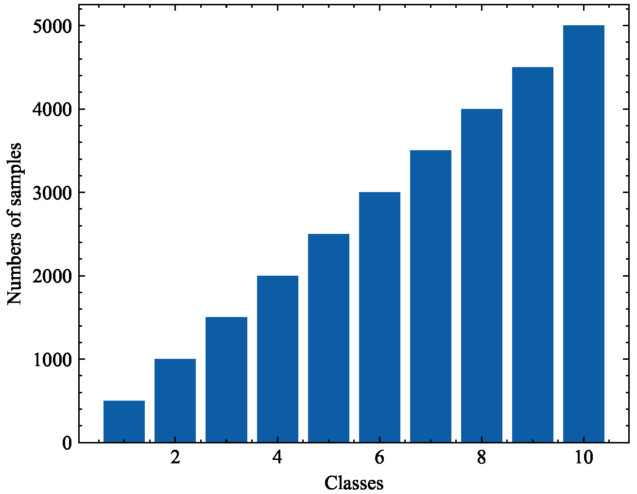
where $N_i$ is a set of examples in class i$(i=2,3,\dots ,C)$ and $\underset{i}{\max }\left\{N_i\right\}$ and $\underset{i}{\min }\left\{N_i\right\}$ return the maximum and minimum class size over all C classes, respectively. The higher the IR value, the larger degree of class imbalance is. Considering that it is a ratio between the maximum and minimum numbers of examples among all classes, the numbers of samples in the remaining classes are interpolated linearly when we artificially reconstruct a dataset, such that the difference between consecutive pairs of classes is constant. An example of linear imbalance distribution with IR = 10 is shown in Figure 3.

3.2. Experiments on Imbalanced MNIST

To verify the generalization and robustness of the proposed CS-BLS, MNIST is adopted in this section. MNIST is a simple dataset and can be used to solve problems that involve digit image classification. The dataset is composed of grayscale images of size $28\times 28$, and it has ten classes corresponding to digits 0 to 9. In the original training dataset, the number of samples per class varies from 5421 in class 5 to 6742 in class 1 [37]. Some example figures of MNIST are shown in Figure 4.

The original training dataset is randomly divided into the training set and validation set. The validation set occupies 10% of the dataset. In an artificially imbalanced version, we uniformly and randomly under-sample each class to contain no more than 5000 examples. The hyperparameters in the experiments are set as follows, which are shown in

Table 1. Hyperparameter settings of CS-BLS and BLS.

Hyperparameter	Value
Imbalance ratio (IR)	5, 10, 25, 50, 100, 250, 500, 1500
Weight decay	0.0005
Learning rate	0.001
Maximum epoch	100
Broad structure	(20, 5, 100), (50, 5, 100), (50, 15, 100), (50, 30, 100), (50, 15, 200)
Nonlinear activation function	tanh

. Experiments on the MNIST dataset are conducted on the following imbalance ratios. For linear imbalance, we test values of $IR\in$ {5, 10, 25, 50, 100, 250, 500, 1500}. The test set of the reconstructed imbalanced dataset has an equal number of instances from each class. We do not alter the test set to match the artificially imbalanced training set. The reason for this is that the score obtained by each classifier on the same test set is straightforward to compare and thus offers accurate performance evaluation.

In the model training process of the CS-BLS methods, we set the weight decay as 0.0005 and the learning rate as 0.001. The classifiers of the CS-BLS methods are iteratively trained with a maximum of 100 epochs, and an early stopping mechanism is used in each classifier. When training CS-BLS methods and the standard BLS method, the number of feature nodes in each set (k), the number of sets of feature nodes (n), and the number of enhancement nodes (p) are set to different numbers, and they are grouped together as (k, n, p) to represent broad structures. The nonlinear activation function ${\xi }_j\left(·\right)$ is a tanh function.

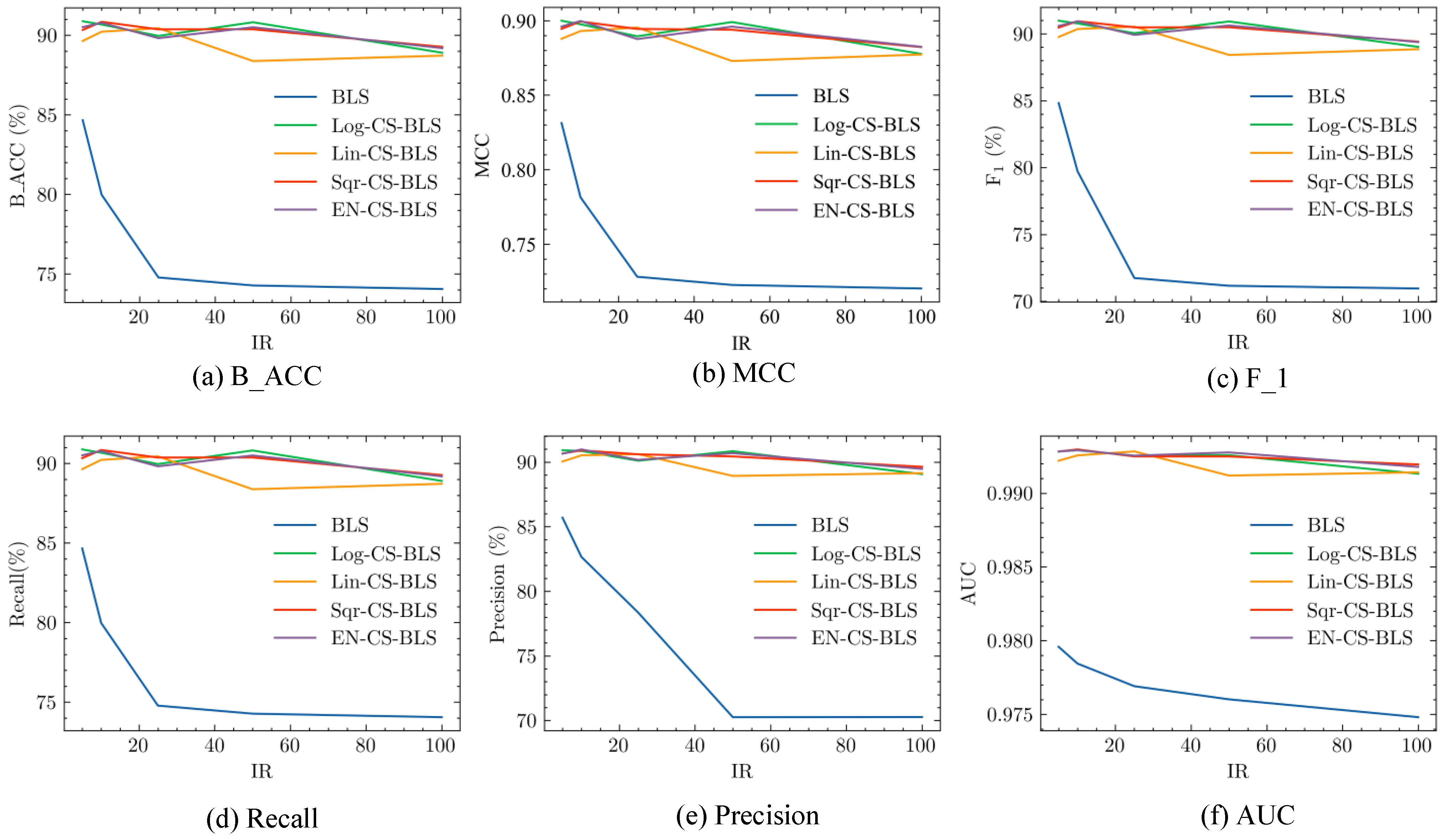
In order to validate the imbalance classification performance of CS-BLS methods on the MNIST dataset with different imbalance ratios, a list of experiments is conducted on the same BLS structure, i.e., (50, 15, 500), and the results are shown in Figure 5. To compare with standard BLS, the results of the standard BLS with the same condition as CS-BLS methods are also shown in Figure 5. From Figure 5, the following findings can be observed.

(1)

Comparison of the standard BLS under different imbalance ratios demonstrates that the performance of the standard BLS gradually decreases as IR increases. Taking B_ACC as an example, it drops from 84.66% (IR = 5) to 74.06% (IR = 100). The other evaluation metrics of standard BLS, as shown in Figure 5, have the same trend as the increase of IR.

(2)

The proposed CS-BLS methods have better performance than the standard BLS on different values of IR. Taking B_ACC and MCC as examples, on average, the B_ACC of the proposed four CS-BLS methods is higher than the standard BLS by 12.30% (5.68–15.74%), and the MCC of the CS-BLS methods and the BLS are 0.8774 (0.8285–0.8974) and 0.7453 (0.7163–0.8312), respectively. The other evaluation metrics of the CS-BLS methods and the BLS show the same pattern as B_ACC and MCC. The results demonstrate the superiority of the CS-BLS methods over the standard BLS in handling imbalanced data.

(3)

It can be found that the performance of different CS-BLS methods is relatively close, and no unique CS-BLS method can achieve the best performance for all the metrics and imbalance ratios.

Furthermore, to verify the performance of the CS-BLS on different broad structures, represented as (k, n, q), several experiments are further conducted for the proposed CS-BLS methods and the standard BLS under different broad structures and the same imbalance ratio (IR = 50). The results are shown in

Table 2. Comparison of proposed CS-BLS methods and standard BLS on imbalanced MNIST with IR = 50 on different broad structures.

Structure	Method	B_ACC	MCC	F${}_1$-Score	Recall	Precision	AUC
(20, 5, 100)	BLS	74.24%	0.7222	0.7110	74.25%	70.32%	0.9766
	Log-CS-BLS	84.29%	0.8276	0.8445	84.29%	85.31%	0.9869
	Lin-CS-BLS	86.47%	0.8517	0.8667	86.47%	86.59%	0.9877
	Sqr-CS-BLS	84.78%	0.8331	0.8504	84.78%	85.54%	0.9865
	EN-CS-BLS	86.69%	0.8541	0.8690	86.69%	87.00%	0.9880
(50, 5, 100)	BLS	74.55%	0.7251	0.7134	74.54%	70.10%	0.9765
	Log-CS-BLS	88.60%	0.8743	0.8871	88.60%	88.79%	0.9907
	Lin-CS-BLS	88.14%	0.8697	0.8820	88.14%	88.33%	0.9901
	Sqr-CS-BLS	88.40%	0.8722	0.8850	88.40%	88.69%	0.9905
	EN-CS-BLS	88.99%	0.8794	0.8905	88.99%	89.15%	0.9909
(50, 15, 100)	BLS	74.32%	0.7230	0.7118	74.32%	70.23%	0.9760
	Log-CS-BLS	89.57%	0.8852	0.8969	89.57%	89.72%	0.9915
	Lin-CS-BLS	88.72%	0.8774	0.8891	88.72%	89.17%	0.9909
	Sqr-CS-BLS	89.83%	0.8884	0.8994	89.83%	89.90%	0.9916
	EN-CS-BLS	89.97%	0.8913	0.9011	89.97%	90.23%	0.9917
(50, 30, 100)	BLS	74.41%	0.7239	0.7126	74.41%	70.17%	0.9757
	Log-CS-BLS	89.74%	0.8885	0.8984	89.74%	90.11%	0.9926
	Lin-CS-BLS	88.38%	0.8733	0.8856	88.38%	89.01%	0.9912
	Sqr-CS-BLS	89.23%	0.8821	0.8937	89.23%	89.49%	0.9914
	EN-CS-BLS	87.72%	0.8671	0.8795	87.72%	88.57%	0.9903
(50, 15, 200)	BLS	74.31%	0.7230	0.7119	74.31%	70.27%	0.9760
	Log-CS-BLS	89.72%	0.8868	0.8981	89.72%	89.78%	0.9919
	Lin-CS-BLS	89.10%	0.8806	0.8914	89.10%	89.31%	0.9913
	Sqr-CS-BLS	89.28%	0.8820	0.8942	89.28%	89.47%	0.9917
	EN-CS-BLS	88.83%	0.8785	0.8893	88.83%	89.21%	0.9915

Remark: Bold means the best result.

. From Table 2, the following findings can be observed.

(1)

In general, the performance of the CS-BLS has improved as the number of feature nodes and enhancement nodes increases to a finite number. Taking B_ACC as an example again, the average B_ACC of the CS-BLS methods increases from 85.56% (84.29–86.69%) on the broad structure (20, 5, 100) to 90.02% (88.38–90.82%) on the broad structure (50, 15, 500). However, the performance of BLS is quite stable at a relatively low value (74.36% on average).

(2)

The proposed CS-BLS has better performance than the standard BLS on each compared broad structure. Taking B_ACC and MCC as examples, on average, the B_ACC of the proposed CS-BLS methods is higher than the standard BLS by 14.31% (11.32–15.74%), and the MCC values of the CS-BLS methods and BLS are 0.8760 (0.8416–0.8904) and 0.7234 (0.7222–0.7239), respectively. The other evaluation metrics of the CS-BLS methods and the BLS show the same pattern as B_ACC and MCC.

(3)

With different broad structures, the performance of the four CS-BLS methods is quite close with a slight variance.

The proposed CS-BLS provides a common framework adopting a cost-sensitive loss function with different calculating methods for penalty weights. Regardless of the methods, all the CS-BLS methods have a better generalization and robustness than the standard BLS. Thus, the proposed framework, i.e., CS-BLS, is effective in imbalanced MNIST.

3.3. Experiments on Imbalanced Small NORB

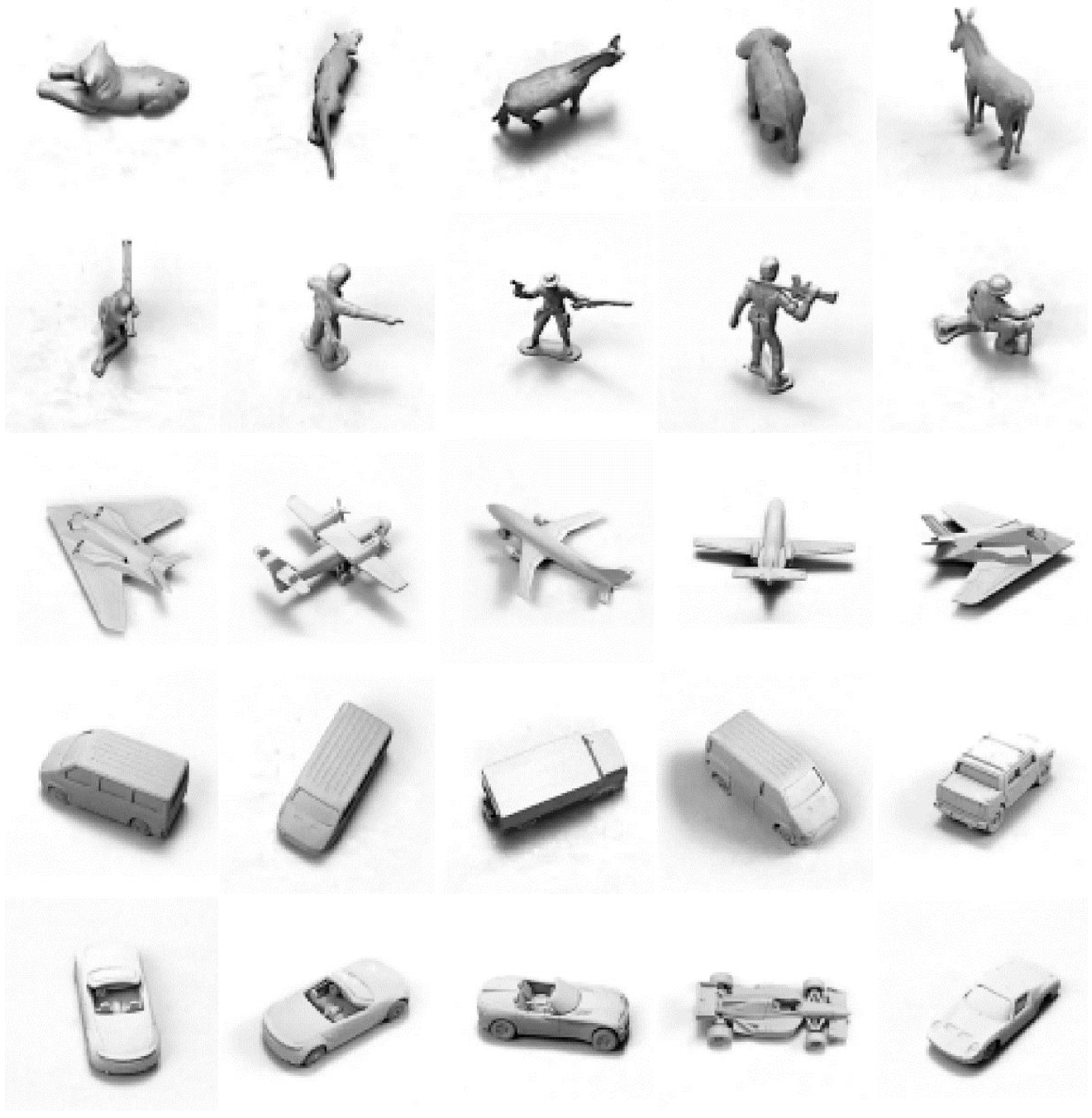
The small NORB dataset is commonly used in 3D object image recognition, and some example figures are shown in Figure 6. It includes images of 50 toys from five general categories: four-legged animals, human figures, airplanes, trucks, and cars. Two cameras captured images of the objects under six different illumination conditions, nine different altitudes (30 to 70 degrees with an interval of 5 degrees), and 18 different azimuths (0 to 340 with an interval of 20 degrees). As the small NORB dataset is a more complex dataset than MNIST, it is adopted to further evaluate the performance of the proposed CS-BLS methods and the standard BLS.

The whole dataset contains ten instances of each category. The training set contains five instances of each category, and the original test set contains the remaining five instances. The original test set is randomly divided into a validation set and test set. The validation set occupies 10% of the original dataset. In artificially imbalanced versions, we uniformly and randomly under-sample each class to contain no more than 4500 examples. Experiments on the small NORB dataset are performed on the following imbalance parameters. For linear imbalance, we test the values of $IR\in$ {5, 10, 25, 50, 100, 250, 500, 1500}. The test set has an equal number of examples in each class.

In the model training process of the CS-BLS methods, all parameters are set the same as the parameters in the previous MNIST experiments, as shown in Table 1. We also use a parameter group (k, n, p), the same as the previous MNIST experiments, to represent broad structures.

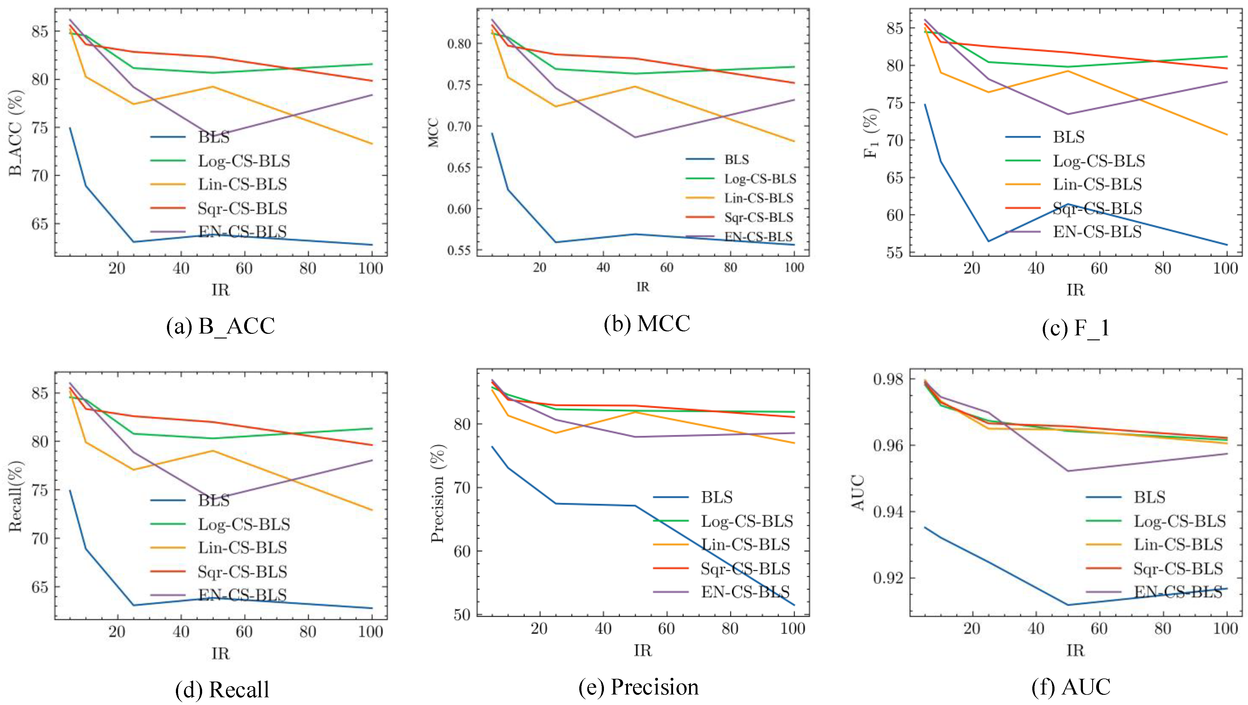
In order to evaluate the imbalance classification performance of the CS-BLS methods and standard BLS on the small NORB dataset with different imbalance ratios, a list of experiments are conducted on the same broad structure, i.e., (50, 15, 500), and the results are shown in Figure 7. From Figure 7, the following findings can be observed.

(1)

The results demonstrate that the performance of the standard BLS gradually decreases as IR increases. Taking B_ACC as an example, it drops from 74.91% (IR = 5) to 62.78% (IR = 100). The other evaluation metrics of standard BLS, as shown in Figure 7, have the same trend as the increase of IR.

(2)

The proposed CS-BLS methods have better performance than the standard BLS on different values of IR. Taking B_ACC and MCC as examples, on average, the B_ACC of the proposed CS-BLS methods is higher than the standard BLS by 12.62% (5.24–17.07%), and the MCC of the CS-BLS and BLS are 0.7350 (0.6222–0.8195) and 0.5869 (0.5552–0.6906), respectively. The other evaluation metrics of the CS-BLS and the BLS show the same pattern as B_ACC and MCC.

(3)

The performance of the four different CS-BLS methods is relatively close, and no unique CS-BLS method can achieve the best performance for all the mentioned imbalance ratios.

Furthermore, to evaluate the performance of the CS-BLS on different broad structures, several experiments are further conducted for the proposed CS-BLS methods and the standard BLS method under different broad structures and the same imbalance ratio (IR = 50). In addition, the corresponding experiments of the standard BLS with the same broad structure and initial parameters are conducted for comparison. The results are shown in

Table 3. Comparison of proposed CS-BLS methods and standard BLS on imbalanced small NORB with IR = 50 on different broad structures.

Structure	Method	B_ACC	MCC	F${}_1$-Score	Recall	Precision	AUC
(20, 5, 100)	BLS	56.33%	0.4750	0.5051	56.33%	47.93%	0.8597
	Log-CS-BLS	59.67%	0.5204	0.5560	58.85%	73.43%	0.9175
	Lin-CS-BLS	66.75%	0.5946	0.6658	66.59%	72.09%	0.9252
	Sqr-CS-BLS	59.47%	0.5156	0.5669	58.71%	71.12%	0.9175
	EN-CS-BLS	67.12%	0.5991	0.6701	66.91%	72.86%	0.9255
(50, 5, 100)	BLS	63.07%	0.5604	0.5653	63.07%	52.40%	0.9125
	Log-CS-BLS	76.87%	0.7165	0.7631	77.18%	78.37%	0.9530
	Lin-CS-BLS	77.16%	0.7146	0.7716	77.08%	77.43%	0.9525
	Sqr-CS-BLS	78.40%	0.7340	0.7822	78.68%	79.66%	0.9528
	EN-CS-BLS	76.34%	0.7063	0.7647	76.19%	77.93%	0.9508
(50, 15, 100)	BLS	62.80%	0.5563	0.5602	62.80%	51.53%	0.9161
	Log-CS-BLS	80.41%	0.7573	0.7996	80.32%	80.62%	0.9581
	Lin-CS-BLS	75.35%	0.6960	0.7496	75.15%	76.51%	0.9464
	Sqr-CS-BLS	78.81%	0.7418	0.7843	78.81%	80.81%	0.9562
	EN-CS-BLS	77.04%	0.7171	0.7695	77.11%	78.67%	0.9537
(50, 30, 100)	BLS	63.51%	0.5658	0.5664	63.51%	52.10%	0.9165
	Log-CS-BLS	85.31%	0.8176	0.8515	85.18%	85.66%	0.9710
	Lin-CS-BLS	74.53%	0.6900	0.7414	74.05%	77.74%	0.9561
	Sqr-CS-BLS	80.49%	0.7598	0.7957	80.05%	81.08%	0.9691
	EN-CS-BLS	76.01%	0.7037	0.7581	75.66%	77.48%	0.9519
(50, 15, 200)	BLS	62.77%	0.5560	0.5599	62.77%	51.50%	0.9165
	Log-CS-BLS	79.88%	0.7502	0.7964	79.70%	80.28%	0.9594
	Lin-CS-BLS	77.45%	0.7249	0.7644	77.40%	78.51%	0.9583
	Sqr-CS-BLS	82.18%	0.7803	0.8217	82.12%	83.35%	0.9649
	EN-CS-BLS	79.47%	0.7453	0.7910	79.32%	79.76%	0.9591

Remark: Bold means the best result.

. From Table 3, the following findings can be observed.

(1)

In general, the performance of the CS-BLS has improved as the number of feature nodes and enhancement nodes increases to a finite number. Taking B_ACC as an example again, the average B_ACC of the CS-BLS increases from 63.25% (59.67–67.12%) on broad structure (20, 5, 100) to 79.74% (77.45–82.18%) on broad structure (50, 15, 200). However, the performance of BLS is quite stable at a relatively low value (61.88% on average).

(2)

The proposed CS-BLS methods have better performance than the standard BLS on each compared broad structure. Taking B_ACC and MCC as examples, the average B_ACC of the proposed CS-BLS methods is higher than the standard BLS by 14.12% (6.92–16.97%), and the MCC of the CS-BLS (on average) and BLS are 0.7060 (0.5574–0.7502) and 0.5449 (0.4750–0.5658), respectively. The other evaluation metrics of the CS-BLS and the BLS show the same pattern as B_ACC and MCC.

(3)

With different broad structures, the performance of the four CS-BLS methods is quite close with a slight variance.

The above results on the small NORB dataset show the same pattern as the experiments on MNIST. As the problem of 3D object recognition on the small NORB dataset is significantly more difficult than the problem of digit image classification on MNIST, the overall performance of the proposed CS-BLS methods and the standard BLS on the small NROB dataset is worse than that on the MNIST dataset. However, we can still draw a conclusion that the proposed CS-BLS framework can improve the performance of BLS on imbalanced classification, and it also demonstrates that the proposed framework, i.e., CS-BLS, is effective.

3.4. Experiments on Breast Ultrasound Cancer Diagnosis

Breast cancer is a serious disease that has become the first most frequent type cancer and the fourth leading cause of cancer-related deaths worldwide, resulting in over 2 million new cases and over 684,000 deaths per year [47]. Breast cancer is a potentially curable disease if it is diagnosed and treated early. The five-year survival rate ranged from 100% (stage I) to 26.5% (stage IV) for female breast cancer [48]. Breast cancer screening is an essential secondary prevention technique for achieving early detection, early diagnosis, and early treatment, due to a lack of effective etiological prevention. Breast ultrasonography produces an image of the interior of the breast using sound waves, and it has been regraded as an effective diagnostic tool because it may detect breast abnormalities, such as fluid-filled cysts.

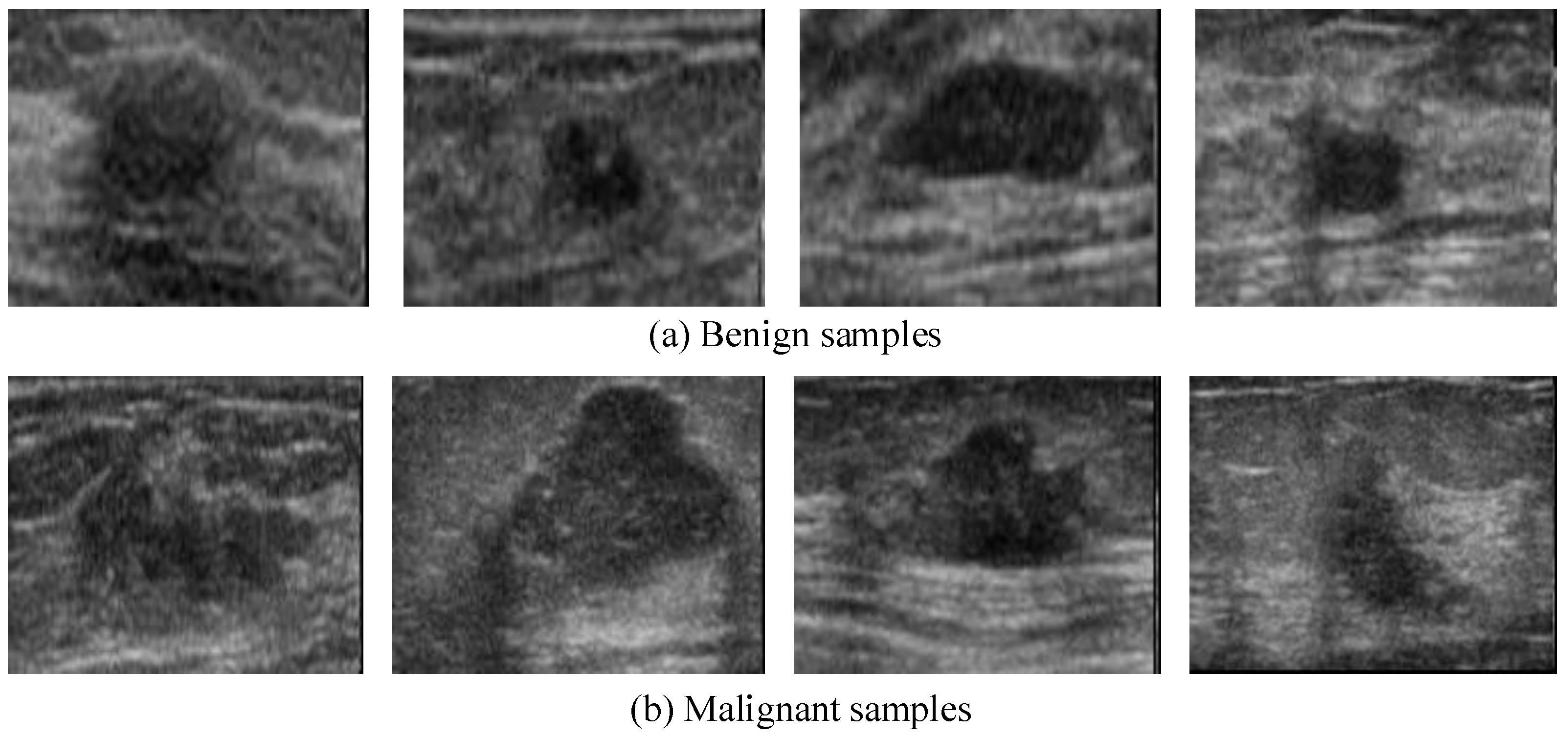
In this section, an open breast ultrasound dataset [12] is adopted to evaluate the proposed CS-BLS on different evaluation metrics. The dataset contains 250 breast ultrasound images, 150 for benign samples and 100 for malignant samples. Example figures in this dataset are shown in Figure 8. The dataset is divided randomly into three parts, 70% for training, 10% for validation, and 20% for testing. To reduce the complexity of the breast ultrasound data, all images are directly resized to 28 × 28. All the hyperparameters on the CS-BLS models are the same as previous settings, as shown in Table 1.

To evaluate the performance of the CS-BLS methods on different broad structures, experiments are conducted under different broad structures. The results are shown in

Table 4. Comparison among the proposed CS-BLS methods on breast ultrasound diagnosis dataset on different broad structures.

Structure	Method	B_ACC	MCC	F${}_1$-Score	Recall	Precision
(20, 5, 100)	BLS	78.00%	0.5618	0.7726	79.17%	77.05%
	Log-CS-BLS	86.00%	0.7290	0.8553	87.85%	85.10%
	Lin-CS-BLS	86.00%	0.7290	0.8553	87.85%	85.10%
	Sqr-CS-BLS	86.00%	0.7005	0.8498	85.42%	84.63%
	EN-CS-BLS	82.00%	0.6281	0.8108	82.29%	80.54%
(50, 5, 100)	BLS	82.00%	0.6003	0.7896	77.43%	82.85%
	Log-CS-BLS	88.00%	0.7622	0.8750	89.41%	86.85%
	Lin-CS-BLS	86.00%	0.7290	0.8553	87.85%	85.10%
	Sqr-CS-BLS	92.00%	0.8335	0.9151	92.53%	90.83%
	EN-CS-BLS	92.00%	0.8335	0.9151	92.53%	90.83%
(50, 15, 100)	BLS	86.00%	0.7005	0.8498	85.42%	84.63%
	Log-CS-BLS	92.00%	0.8335	0.9151	92.53%	90.83%
	Lin-CS-BLS	92.00%	0.8335	0.9151	92.53%	90.83%
	Sqr-CS-BLS	96.00%	0.9132	0.9566	95.66%	95.66%
	EN-CS-BLS	92.00%	0.8335	0.9151	92.53%	90.83%
(50, 30, 100)	BLS	84.00%	0.6528	0.8264	82.64%	82.64%
	Log-CS-BLS	96.00%	0.9186	0.9576	96.88%	95.00%
	Lin-CS-BLS	98.00%	0.9580	0.9785	98.44%	97.37%
	Sqr-CS-BLS	96.00%	0.9132	0.9566	95.66%	95.66%
	EN-CS-BLS	96.00%	0.9132	0.9566	95.66%	95.66%
(50, 15, 200)	BLS	88.00%	0.7396	0.8698	86.98%	86.98%
	Log-CS-BLS	92.00%	0.8335	0.9151	92.53%	90.83%
	Lin-CS-BLS	94.00%	0.8722	0.9356	94.10%	93.12%
	Sqr-CS-BLS	94.00%	0.8722	0.9356	94.10%	93.12%
	EN-CS-BLS	96.00%	0.9132	0.9566	95.66%	95.66%

Remark: Bold means the best result.

. From Table 4, the following findings can be observed.

(1)

In general, the performance of the CS-BLS is improved as the number of hidden nodes increases to a finite number. Taking B_ACC as an example again, the average B_ACC of the CS-BLS increases from 85.00% (82.00–86.00%) on broad structure (20, 5, 100) to 96.50% (96.00–98.00%) on broad structure (50, 30, 100). The other evaluation metrics show the same pattern with B_ACC.

(2)

With different broad structures, the performance of the four CS-BLS methods is quite close with little variance.

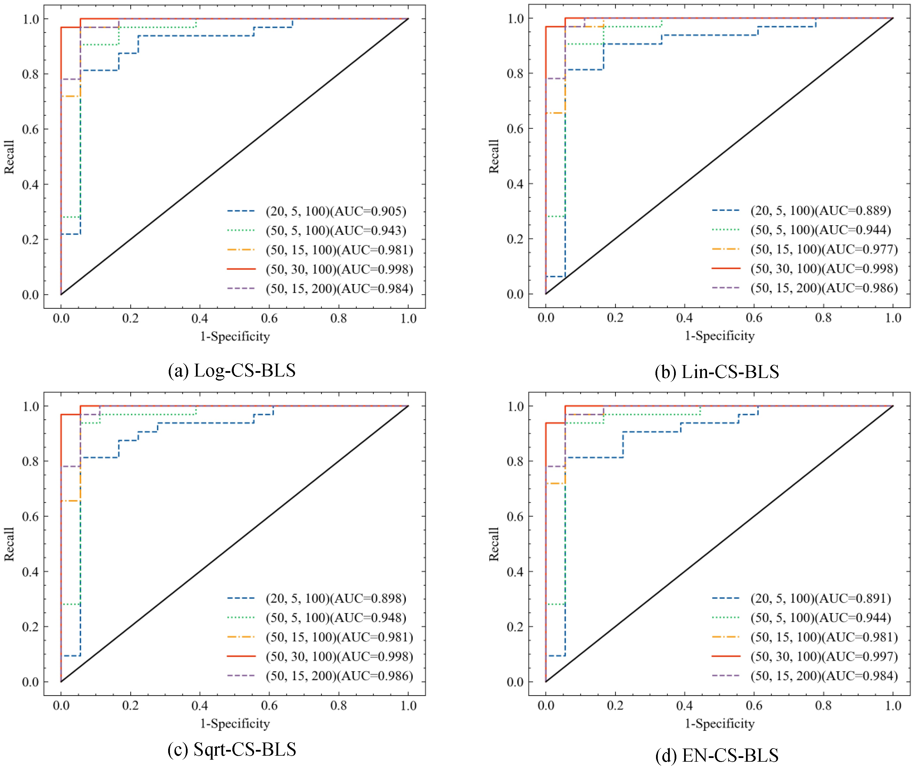
To evaluate the proposed CS-BLS methods on diagnosis results, four ROC figures of CS-BLS methods are demonstrated on different broad structures, as shown in Figure 9. The specificity in Figure 9 is a measure of how well a test can identify TNs. The results show the good performance of the proposed CS-BLS methods, especially when larger feature nodes and enhancement nodes are set. The results also indicate that the CS-BLS methods enable an accurate and reliable breast ultrasound cancer diagnosis.

4. Discussion

The imbalanced classification problem, which suffers from imbalanced class distribution, is commonly encountered in real-world applications. We have proposed a novel cost-sensitive BLS, CS-BLS, to improve the ability of BLS to handle it. Four different CS-BLS methods have been proposed: Log-CS-BLS, Lin-CS-BLS, Sqr-CS-BLS, and EN-CS-BLS, respectively, corresponding to four different weighted penalty factor calculation methods. With systemic experimental studies, the results show that the CS-BLS performs better than the BLS in dealing with imbalanced data, no matter whether in the imbalanced MNIST dataset, the imbalanced small NORB dataset, or the breast ultrasound diagnosis dataset.

BLS is an effective and efficient machine learning method in many tasks. However, as the weight matrix of BLS is calculated based on the ridge regression approximation, which is based on MMSE, the BLS is inherently inappropriate for solving imbalanced classification problems. In general, there are three levels of methods to handle imbalanced data: the data level, the classifier level, and the hybrid level. However, not much research has been done on BLS handling imbalanced data. In this paper, we propose a novel classifier-level framework, CS-BLS, which can adapt to different loss functions, allowing it to integrate with existing advanced methods for imbalanced data. We only conducted experiments on the framework with the loss function of WCE, and other loss functions may achieve better performance integrated with the CS-BLS framework, such as MFE [30], MSFE [30], and FL [31]. We will explore these loss functions on the CS-BLS framework in our future work. The images in the three used datasets are relatively simple for classifiers to learn, and the CS-BLS may encounter difficulties when processing the image data with high resolution. Other advanced techniques can be adopted in this framework when encountering high-resolution images. Firstly, deep auto-encoders [49] can be used to reduce dimensionality and obtain low-dimensional features. Secondly, transfer learning with pre-trained weights [50] can also be used to extract features for the CS-BLS, which can be processed by feature reduction methods, such as principal component analysis (PCA), to obtain low-dimensional features.

Regarding the time complexity of the proposed CS-BLS and BLS, we analyze them qualitatively in two aspects, i.e., training time complexity and exploitation time complexity. Firstly, on the exploitation time complexity, since our proposed CS-BLS algorithm and the standard BLS only differentiate from loss functions, they lead to different weight matrices with the same dimension. Thus, the exploitation time complexity of both is the same. Secondly, on the training time complexity, we compare the training time of both. Taking MNIST as an example, the training time of BLS is 0.68 s when IR = 50 and the broad network is (20, 5, 100). While keeping IR constant, the training time increases gradually as the broad network increases. When the broad networks are (50, 5, 100), (50, 15, 100), (50, 15, 200), and (50, 30, 100), the training times are 1.15 s, 3.10 s, 3.34 s, and 6.30 s, respectively. The training time of CS-BLS remains 43–45 s in the same condition of IR and broad network, because we limit the maximum number of epochs and use the early stopping mechanism. Thus, the training time of the proposed CS-BLS is longer than that of BLS, although it is within an acceptable range. However, the performance of CS-BLS is much better than that of BLS, as shown in the previous analysis in Section 3.

5. Conclusions

BLS is an effective and efficient method, and it has received attention from many researchers due to its outstanding performance. To improve the ability of BLS for handling imbalanced data, a novel BLS, called CS-BLS, is proposed. The weighted penalty factor in the CS-BLS is utilized to provide a proper weight to each sample and constrain its contribution. Samples in minor classes are assigned greater weights to raise their contributions in modeling, whereas samples in major classes are assigned lower weights to reduce their contributions. Four calculation methods for weighted penalty factors are applied for CS-BLS, and thus, four kinds of CS-BLS approaches are constructed: Log-CS-BLS, Lin-CS-BLS, Sqr-CS-BLS, and EN-CS-BLS. Systematic experiments on four CS-BLS methods and the standard BLS are conducted under different imbalance ratios and different broad structures on two commonly used datasets, i.e., MNIST and small NORB, to demonstrate the effectiveness and robustness of the proposed methods. The results demonstrate that the CS-BLS approaches perform better than the standard BLS in all the experiments. Finally, the proposed CS-BLS methods are applied to a clinical breast ultrasound dataset, and the results indicate accurate and reliable diagnostic results on breast cancer.

References

- Chen, C.L.P.; Liu, Z. Broad learning system: An effective and efficient incremental learning system without the need for deep architecture. IEEE Trans. Neural Netw. Learn. Syst. 2017, 29, 10–24. [Google Scholar] [CrossRef]
- Pao, Y.H.; Park, G.H.; Sobajic, D.J. Learning and generalization characteristics of the random vector functional-link net. Neurocomputing 1994, 6, 163–180. [Google Scholar] [CrossRef]
- Wong, P.K.; Yao, L.; Yan, T.; Choi, I.C.; Yu, H.H.; Hu, Y. Broad learning system stacking with multi-scale attention for the diagnosis of gastric intestinal metaplasia. Biomed. Signal Process. Control 2022, 73, 103476. [Google Scholar] [CrossRef]
- Jiang, S.B.; Wong, P.K.; Guan, R.; Liang, Y.; Li, J. An efficient fault diagnostic method for three-phase induction motors based on incremental broad learning and non-negative matrix factorization. IEEE Access 2019, 7, 17780–17790. [Google Scholar] [CrossRef]
- Huang, H.; Zhang, T.; Yang, C.; Chen, C.P. Motor learning and generalization using broad learning adaptive neural control. IEEE Trans. Ind. Electron. 2019, 67, 8608–8617. [Google Scholar] [CrossRef]
- Xu, L.; Chen, C.L.P.; Han, R. Sparse Bayesian Broad Learning System for Probabilistic Estimation of Prediction. IEEE Access 2020, 8, 56267–56280. [Google Scholar] [CrossRef]
- Feng, S.; Chen, C.P. Broad learning system for control of nonlinear dynamic systems. In Proceedings of the 2018 IEEE International Conference on Systems, Man, and Cybernetics (SMC), Miyazaki, Japan, 7–10 October 2018; pp. 2230–2235. [Google Scholar]
- Huang, C.; Huang, X.; Fang, Y.; Xu, J.; Qu, Y.; Zhai, P.; Fan, L.; Yin, H.; Xu, Y.; Li, J. Sample imbalance disease classification model based on association rule feature selection. Pattern Recognit. Lett. 2020, 133, 280–286. [Google Scholar] [CrossRef]
- Gao, X.; Chen, Z.; Tang, S.; Zhang, Y.; Li, J. Adaptive weighted imbalance learning with application to abnormal activity recognition. Neurocomputing 2016, 173, 1927–1935. [Google Scholar] [CrossRef]
- Zhao, B.; Zhang, X.; Li, H.; Yang, Z. Intelligent fault diagnosis of rolling bearings based on normalized CNN considering data imbalance and variable working conditions. Knowl.-Based Syst. 2020, 199, 105971. [Google Scholar] [CrossRef]
- Somasundaram, A.; Reddy, S. Parallel and incremental credit card fraud detection model to handle concept drift and data imbalance. Neural Comput. Appl. 2019, 31, 3–14. [Google Scholar] [CrossRef]
- Rodrigues, P.S. Breast Ultrasound Image. Mendeley Data 2018. [Google Scholar] [CrossRef]
- Kaur, H.; Pannu, H.S.; Malhi, A.K. A Systematic Review on Imbalanced Data Challenges in Machine Learning: Applications and Solutions. ACM Comput. Surv. 2019, 52, 1–36. [Google Scholar] [CrossRef] [Green Version]
- Leevy, J.L.; Khoshgoftaar, T.M.; Bauder, R.A.; Seliya, N. A survey on addressing high-class imbalance in big data. J. Big Data 2018, 5, 42. [Google Scholar] [CrossRef]
- Johnson, J.M.; Khoshgoftaar, T.M. Survey on deep learning with class imbalance. J. Big Data 2019, 6, 27. [Google Scholar] [CrossRef]
- Vitter, J.S. Random sampling with a reservoir. ACM Trans. Math. Softw. 1985, 11, 37–57. [Google Scholar] [CrossRef] [Green Version]
- Chawla, N.V.; Bowyer, K.W.; Hall, L.O.; Kegelmeyer, W.P. SMOTE: Synthetic minority over-sampling technique. J. Artif. Intell. Res. 2002, 16, 321–357. [Google Scholar] [CrossRef]
- Chen, S.; He, H.; Garcia, E.A. RAMOBoost: Ranked minority oversampling in boosting. IEEE Trans. Neural Netw. 2010, 21, 1624–1642. [Google Scholar] [CrossRef]
- He, H.; Bai, Y.; Garcia, E.A.; Li, S. ADASYN: Adaptive synthetic sampling approach for imbalanced learning. In Proceedings of the 2008 IEEE International Joint Conference on Neural Networks, Hong Kong, China, 1–8 June 2008; pp. 1322–1328. [Google Scholar]
- Han, H.; Wang, W.Y.; Mao, B.H. Borderline-SMOTE: A new over-sampling method in imbalanced data sets learning. In Proceedings of the International Conference on Intelligent Computing (ICIC), Hefei, China, 23–25 August 2005; pp. 878–887. [Google Scholar]
- Barua, S.; Islam, M.M.; Yao, X.; Murase, K. MWMOTE–Majority weighted minority oversampling technique for imbalanced data set learning. IEEE Trans. Knowl. Data Eng. 2012, 26, 405–425. [Google Scholar] [CrossRef]
- Lin, W.C.; Tsai, C.F.; Hu, Y.H.; Jhang, J.S. Clustering-based undersampling in class-imbalanced data. Inf. Sci. 2017, 409, 17–26. [Google Scholar] [CrossRef]
- Barandela, R.; Rangel, E.; Sánchez, J.S.; Ferri, F.J. Restricted decontamination for the imbalanced training sample problem. In Proceedings of the Iberoamerican Congress on Pattern Recognition, Havana, Cuba, 26–29 November 2003; pp. 424–431. [Google Scholar]
- Zheng, Y.D.; Liu, Z.; Lu, T.; Wang, L. Dynamic sampling networks for efficient action recognition in videos. IEEE Trans. Image Process. 2020, 29, 7970–7983. [Google Scholar] [CrossRef]
- Fu, B.; He, J.; Zhang, Z.; Qiao, Y. Dynamic Sampling Network for Semantic Segmentation. In Proceedings of the AAAI Conference on Artificial Intelligence (AAAI), Midtown, NY, USA, 7–12 February 2020; Volume 34, pp. 10794–10801. [Google Scholar]
- Zong, W.; Huang, G.B.; Chen, Y. Weighted extreme learning machine for imbalance learning. Neurocomputing 2013, 101, 229–242. [Google Scholar] [CrossRef]
- Krawczyk, B.; Woźniak, M.; Schaefer, G. Cost-sensitive decision tree ensembles for effective imbalanced classification. Appl. Soft Comput. 2014, 14, 554–562. [Google Scholar] [CrossRef] [Green Version]
- Aurelio, Y.S.; de Almeida, G.M.; de Castro, C.L.; Braga, A.P. Learning from imbalanced data sets with weighted cross-entropy function. Neural Process. Lett. 2019, 50, 1937–1949. [Google Scholar] [CrossRef]
- Wong, M.L.; Seng, K.; Wong, P.K. Cost-sensitive ensemble of stacked denoising autoencoders for class imbalance problems in business domain. Expert Syst. Appl. 2020, 141, 112918. [Google Scholar] [CrossRef]
- Wang, S.; Liu, W.; Wu, J.; Cao, L.; Meng, Q.; Kennedy, P.J. Training deep neural networks on imbalanced data sets. In Proceedings of the 2016 International Joint Conference on Neural Networks (IJCNN), Vancouver, BC, Canada, 24–29 July 2016; pp. 4368–4374. [Google Scholar]
- Lin, T.Y.; Goyal, P.; Girshick, R.; He, K.; Dollár, P. Focal loss for dense object detection. In Proceedings of the IEEE International Conference on Computer Vision (ICCV), Venice, Italy, 22–29 October 2017; pp. 2980–2988. [Google Scholar]
- Liu, X.Y.; Wu, J.; Zhou, Z.H. Exploratory undersampling for class-imbalance learning. IEEE Trans. Syst. Man Cybern. Cybern. 2008, 39, 539–550. [Google Scholar]
- Chawla, N.V.; Lazarevic, A.; Hall, L.O.; Bowyer, K.W. SMOTEBoost: Improving prediction of the minority class in boosting. In Proceedings of the European Conference on Principles of Data Mining and Knowledge Discovery (PKDD), Cavtat-Dubrovnik, Croatia, 22–26 September 2003; pp. 107–119. [Google Scholar]
- Havaei, M.; Davy, A.; Warde-Farley, D.; Biard, A.; Courville, A.; Bengio, Y.; Pal, C.; Jodoin, P.M.; Larochelle, H. Brain tumor segmentation with deep neural networks. Med. Image Anal. 2017, 35, 18–31. [Google Scholar] [CrossRef] [Green Version]
- Malakar, S.; Ghosh, M.; Bhowmik, S.; Sarkar, R.; Nasipuri, M. A GA based hierarchical feature selection approach for handwritten word recognition. Neural Comput. Appl. 2020, 32, 2533–2552. [Google Scholar] [CrossRef]
- Bacanin, N.; Stoean, R.; Zivkovic, M.; Petrovic, A.; Rashid, T.A.; Bezdan, T. Performance of a novel chaotic firefly algorithm with enhanced exploration for tackling global optimization problems: Application for dropout regularization. Mathematics 2021, 9, 2705. [Google Scholar] [CrossRef]
- LeCun, Y.; Bottou, L.; Bengio, Y.; Haffner, P. Gradient-based learning applied to document recognition. Proc. IEEE 1998, 86, 2278–2324. [Google Scholar] [CrossRef] [Green Version]
- Zhang, T.L.; Chen, R.; Yang, X.; Guo, S. Rich feature combination for cost-based broad learning system. IEEE Access 2018, 7, 160–172. [Google Scholar] [CrossRef]
- Chu, F.; Liang, T.; Chen, C.P.; Wang, X.; Ma, X. Weighted broad learning system and its application in nonlinear industrial process modeling. IEEE Trans. Neural Netw. Learn. Syst. 2019, 31, 3017–3031. [Google Scholar] [CrossRef]
- Zhang, T.; Li, Y.; Chen, R. Evolutionary-Based Weighted Broad Learning System for Imbalanced Learning. In Proceedings of the 2019 IEEE 14th International Conference on Intelligent Systems and Knowledge Engineering (ISKE), Dalian, China, 14–16 November 2019; pp. 607–615. [Google Scholar]
- Gan, M.; Zhu, H.T.; Chen, G.Y.; Chen, C.P. Weighted generalized cross-validation-based regularization for broad learning system. IEEE Trans. Cybern. 2020, 1–9. [Google Scholar] [CrossRef]
- Yang, K.; Yu, Z.; Chen, C.P.; Cao, W.; You, J.J.; San Wong, H. Incremental Weighted Ensemble Broad Learning System For Imbalanced Data. IEEE Trans. Knowl. Data Eng. 2021. [Google Scholar] [CrossRef]
- Zheng, Y.; Chen, B.; Wang, S.; Wang, W. Broad Learning System Based on Maximum Correntropy Criterion. IEEE Trans. Neural Netw. Learn. Syst. 2020, 32, 3083–3097. [Google Scholar] [CrossRef]
- Chen, G.; Choi, W.; Yu, X.; Han, T.; Chandraker, M. Learning efficient object detection models with knowledge distillation. In Proceedings of the 31st International Conference on Neural Information Processing Systems (NIPS), Long Beach, CA, USA, 4–9 December 2017; pp. 742–751. [Google Scholar]
- Lertnattee, V.; Theeramunkong, T. Analysis of inverse class frequency in centroid-based text classification. In Proceedings of the IEEE International Symposium on Communications and Information Technology (ISCIT), Sapporo, Japan, 26–29 October 2004; Volume 2, pp. 1171–1176. [Google Scholar]
- Cui, Y.; Jia, M.; Lin, T.Y.; Song, Y.; Belongie, S. Class-balanced loss based on effective number of samples. In Proceedings of the IEEE/CVF Conference on Computer Vision and Pattern Recognition (CVPR), Long Beach, CA, USA, 15–20 June 2019; pp. 9268–9277. [Google Scholar]
- Sung, H.; Ferlay, J.; Siegel, R.L.; Laversanne, M.; Soerjomataram, I.; Jemal, A.; Bray, F. Global cancer statistics 2020: GLOBOCAN estimates of incidence and mortality worldwide for 36 cancers in 185 countries. CA Cancer J. Clin. 2021, 71, 209–249. [Google Scholar] [CrossRef]
- Cronin, K.A.; Lake, A.J.; Scott, S.; Sherman, R.L.; Noone, A.M.; Howlader, N.; Henley, S.J.; Anderson, R.N.; Firth, A.U.; Ma, J.; et al. Annual Report to the Nation on the Status of Cancer, Part I: National Cancer Statistics. Cancer 2018, 124, 2785–2800. [Google Scholar] [CrossRef] [Green Version]
- Chen, M.; Shi, X.; Zhang, Y.; Wu, D.; Guizani, M. Deep feature learning for medical image analysis with convolutional autoencoder neural network. IEEE Trans. Big Data 2017, 7, 750–758. [Google Scholar] [CrossRef]
- Kermany, D.S.; Goldbaum, M.; Cai, W.; Valentim, C.C.S.; Liang, H.; Baxter, S.L.; Mckeown, A.; Yang, G.; Wu, X.; Yan, F. Identifying Medical Diagnoses and Treatable Diseases by Image-Based Deep Learning. Cell 2018, 172, 1122–1131. [Google Scholar] [CrossRef]
Figure 1.
Standard BLS structure. The input data () are firstly processed with randomly initialized weights ( and ) and a series of activation functions () to produce feature nodes. Then, feature nodes are mapped to enhancement nodes with another set of random weights ( and ) and a series of nonlinear activation functions ().
Figure 2.
Balanced accuracy of BLS decreases as imbalance ratio increases.
Figure 3.
An example of linear imbalance distribution with IR = 10. The number of class samples in class 10 (i.e., 5000) is ten times the number of class samples in class 1 (i.e., 500).
Figure 4.
Example figures in the MNIST dataset. The dataset consists of grayscale images of size , and there are ten classes corresponding to digits from 0 to 9.
Figure 5.
Performance comparison among CS-BLS methods and BLS on the MNIST dataset with different IRs. Six evaluation metirics are compared separately among the five methods.
Figure 6.
Example figures in the small NORB dataset, and they are four-legged animals, human figures, airplanes, trucks, and cars, respectively.
Figure 7.
Performance comparison among CS-BLS methods and BLS on the small NORB dataset with different IRs. Six evaluation metirics are compared separately among the five methods.
Figure 8.
Example figures in the US breast diagnosis dataset. The dataset contains 250 breast ultrasound images, 150 for benign samples and 100 for malignant samples.
Figure 9.
ROCs of four CS-BLS methods under different broad structures.