Introducing The MoreyBall Coefficient

I’ve been obsessed with shooting zones on a basketball court since I was a young boy. Okay, maybe not a young boy, but I did do a study on the subject a few years ago. At that time, my goal was to create a version of true shooting percentage that accounted for specific values of shots from different locations on the court. We know at a basic points per shot level that not all zones on the court are created equal. Not every two-point field goal attempt is the same nor are every three-point field goal attempt. Shooting at the rim and the free throw line, for example, have a higher points per shot value than short and long midrange shooting.

Because of this mathematical reality, my goal was to control for and take into account these differences. Shouldn’t a player be “rewarded” or “punished” for taking “better” or “worse” shots? Moreover, is it possible to have one statistic that helps explain a player’s shot profile instead of diving into individual shot charts? I still believe that these are fair questions to ask.

No matter the nuance, this is fairly obvious, Basketball 101 type stuff I’m talking about here. However, it is always nice to have some sort of mathematical backing to what’s known already. It’s like a warm, cashmere sweater from Madewell caressing your skin ever-so softy (Editor note: this article was not sponsored by Madewell, but if they want to sponsor Drew and send him free clothes, go for it).

With the help of Ryan Davis’ fantastic NBA Shot Charts website, I was finally able to construct the actual analysis I’ve always wanted to perform on NBA Stats’ shooting zone data. Let me introduce the MoreyBall Coefficient (MBC) and the MoreyBall Shot Coefficient (MBSC).

Methodology

So, what exactly are MBC & MBSC? What type of insane “analytics” did you perform in order to create another dumb-butt “advanced stat” that is useless? These are all very valid questions, NBA Eye Test Twitter. The methodology is rather straightforward. I used a five-year luck-adjusted offensive RAPM (LA ORAPM) from 2014–19 as the dependent variable and performed a regression with the different shooting zones as the explanatory variables (more on the zones a few paragraphs down).

If you’re not familiar with RAPM, here is a link to read up on it. If you’re not familiar with luck-adjusted metrics, click on the “Luck Adjusted RAPM” tab in this link and then click the “Expand” box.

The “too-long; didn’t read” definition of RAPM is that it is simply adjusted plus-minus run with a ridge regression instead of an OLS (ordinary least squares) regression because ridge regressions minimize standard errors and help control for heteroskedasticity and multicollinearity (read this article for definitions of these terms).

Okay, maybe that’s not the best layman's terms for RAPM. The term stands for “regularized adjusted plus-minus” Regularization is an aspect of a ridge regression that does not matter to this specific discussion, but understanding the difference between ridge and OLS regressions is important. One of the reasons why we would use a ridge regression for an analysis — and the one most important for plus-minus data — is that the predictor variables are highly correlated.

Let me use this hypothetical to explain: Say I want to measure what stats effect the variation in defensive RAPM and I use players’ steals and forced turnovers in the same study. Because steals are “force turnovers,” these two predictor variables will measure the same phenomena. With lineup data of raw plus-minus differentials, you can’t completely parse out each individual player. Because of this, certain players may be effecting the same phenomena on the court. OLS regression does not do deal with multicollinearity and it can cause wonky standard errors, making a study useless. Running ridge regression on raw lineup data was one of the most important methodologies of the basketball analytics movement.

The “too-long; didn’t read” definition of luck-adjusted RAPM is that it’s RAPM but uses career shooting averages from zones to calculate an expected point differential versus the actual point differential. For example, if Julius Randle goes off for a 20-game stretch where he is 69 percent on 3-pointers but is a career 20 percent shooter from three (don’t know if that’s actually true and don’t care. It feels right), luck adjustments use the 20 percent career figure instead of the 69 percent figure. How I feel about luck adjusted figures requires a whole other article, but it’s actually the better version of RAPM to use when measuring shooting figures over a five-year stretch.

RAPM is certainly not perfect, but its lack of box score elements in its calculation makes it a perfect resource to measure the statistical impact of certain aspects of basketball.

The reason I used a five-year sample instead of a year-over-year sample is because shooting, especially three-point shooting, varies quite a bit and needs a large sample to stabilize. In case you do not want to read Darryl Blackport’s article I linked in the previous sentence, here is the important paragraph:

One season isn’t enough. Even if you have multiple single-seasons, when you’re analyzing shooting, you need a large, collective sample. Therefore, in conjunction with the five-year luck adjusted offensive RAPM, I took the shooting zone totals from NBA Stats — restricted area, paint non-restricted area, midrange, corner three, above the break three — of that five-year sample and summed up the totals for each player. From there, I converted those five-year total numbers to per-48-minute variables to both standardize and control for minutes. If I had five-year possession totals, I would have converted the figures to per-100 possession values. This approach is not dissimilar from how DRE or PIPM were created.

Once I converted my shooting variables into per-48 versions of themselves, I then calculated a “shot volume standard deviation dummy” variable to control for volume shooting. This was suggested by the homie Ben Taylor to me on Twitter last year when I was doing exploratory analysis on the subject. The dummy variable’s creation is quite simple: calculate the data set’s total shot attempts per-48 average and standard deviation, and then assign numbers to represent how many standard deviations above or below the mean the player is for his total shot attempts per-48. For example, if the mean is 15.0 total shot attempts per-48 (I’m too lazy to look at the original data) and the standard deviation is 4.0, players who average over 23.0 total shot attempts (two standard deviations above the mean) received the value “2” while players who average under 11.0 (one standard deviation under the mean) received the value “-1”. Simple enough, right?

Once I got my numbers all calculated, I then removed from the sample players who did not play at least 100 minutes over this five-year period. The reason for removing those low-minutes players is because all those zeroes they have for shooting attempts and shots made can mess up the results of a regression. I wanted to keep some low-minutes players in this analysis, but not so low that they skew the results in a bad way.

Below is a cleaned-up version of my OLS regression on five-year luck-adjusted offensive RAPM with the 13 explanatory variables:

There is some statistic jargon that’s about to follow this sentence but I swear an explanation will follow. With an overall p-value of 0.00 and an r-squared value of 0.32, the model at large is statistically significant and explains 32 percent of the dependent variable’s (LA ORAPM) variation. This makes sense given that offense isn’t just about shooting. The p-values for almost all the explanatory variables are also great and at levels of statistical significance your econometrics professor would love. Ideally, you want the p-value to be less than or equal to 0.05, but since this is just a blog on basketball and not a journal submission to statistics academia, I’m taking the 91 percent confidence level for restricted area shot attempts and 94 percent confidence level for paint non-restricted area shot attempts as victories. I mean, they actually are good values, just not ideal.

Oh, before I forget, confidence levels are calculated by subtracting the p-value from one and then multiplying by 100 to convert to a percentage — (1-0.01) x 100 would be 99 percent. Another way to measure the significance of an explanatory variable is the t-value. If a t-value is greater than or equal to +2 or -2, that is ideal. For most econometric heads, the -1.68 and the -1.89 t-values for paint non-restricted shot and attempts and midrange attempts don’t fit that criteria, but it’s close enough. Cut me some slack!

I should probably dive more into why the shot volume dummy is not statistically significant, but I wouldn’t be concerned too much given that it was mainly as a control for the overall study. What is actually strange is the corner three shot attempts variable not being statistically significant. Hopefully Ben Taylor or one of my other Nylon Calculus buddies are reading this and will reach out to tell me what’s going on. Or maybe some data dork that is a Knicks fan who reads the greatest Knicks website on the Internet will help explain the situation. The conclusion I come to is that you can more or less jack up as many corner threes as you want since there is no statistically significant negative effect. There isn’t a positive effect either, but if you’re making corner threes, you’re golden.

So let’s go over the coefficient results. The shots made zones order from highest coefficient to lowest coefficient:

1. Above the break threes (+1.13)
2. Corner threes (+0.82)
3. Midrange (+0.65)
4. Free throws (+0.63)
5. Paint non-restricted area (+0.60)
6. Restricted area (+0.37)

You’re probably asking what do coefficients do? Great question, anonymous reader. Let’s use midrange shots made as an example. For every unit increase in midrange shots made while holding all other variables constant, luck-adjusted offensive RAPM increases +0.65. It’s surprisingly straightforward. What these results are telling us is that if you’re making threes, midrange shots, free throws, and that short midrange area at a high rate, you as a player will have a high projected LA OPRAPM.

But Drew, you said that shots at the rim are super efficient in terms of points per shot?! Why isn’t the coefficient higher for restricted area shots made? Another great question. One thing to keep in mind is that shots in the restricted area are the most taken shot in the NBA, and the sheer volume does suppress the coefficient a bit. With that said, let’s get to the shot attempts part of this analysis because this is where shots at the rim become super important. Here is the breakdown of the coefficients for the shots attempted from least to highest:

1. Restricted area (-0.16)
2. Above the break threes (-0.21)
3. Free throws (-0.25)
4. Paint non-restricted area (-0.25)
5. Midrange (-0.31)

I’m not including the corner threes because they aren’t statistically significant. If that -0.08 figure was, it would be atop the list. What this is telling us is that when holding all other variables constant, restricted area shots attempted have the least negative effect while midrange shots attempted have the highest negative effect. Another way to frame this conclusion is that if you’re a player who is primarily getting to the rim, taking and missing these shots at a higher rate will not be as bad if you were taking and missing midrange shots at a higher rate. This is why teams like the Bucks and Knicks focus so much on taking away shots at the rim. Given the high variability of three-point shooting game-to-game and the high penalty for taking midrange shots, you want teams shooting outside the paint as much as possible since it will give you the best chance of winning.

To calculate both MBC and MBSC, I use a regression equation to determine the values. For the stats dorks reading this, MBC is a projected LA ORAPM using the 12 shooting zone coefficients and MBSC is a projected LA ORAPM using the six shots attempted coefficients. The formula is the sum of the intercept (-1.77) and each variable’s per-48 figure times the respective coefficient value.

Results

Since this is a Knicks website, I’ll begin with the current results of the team. Now with the NBA season effectively canceled because of COVID-19, these will be the final numbers.

No surprise that in his limited minutes, Allonzo Trier has the best MBC on the team. He would fit well with Houston coming off the bench and why a deal couldn’t be struck at the deadline is beyond me. But let’s table that discussion. The MBSC results are actually what is intriguing to me given that the Knicks overall aren’t an efficient offense, hence the lower MBC figures. Julius Randle and RJ Barrett have the best MBSC figures on the team. This tells us that they have a good shot profile, but simply aren’t efficient enough to minimize the penalties for taking the shots and missing. This is actually very promising for Barrett because he will more than likely increase his efficiency as he gets older and doesn’t play with a lineup with clogged toilet spacing.

You’re probably wondering why Mitchell Robinson’s MBC and MBSC figures are so low since “shots at the rim are good.” The one thing that the MoreyBall Coefficient does is truly reward hyper-efficient players who effectively only take threes and shots at the rim. When you look at all the data in a moment, you will see where the bias lies. Robinson isn’t a volume shooter and takes an estimated 200 percent of his shots at the rim. Translation, despite being efficient and fitting the profile of a rim-running, MoreyBall center, Robinson’s lack of volume and three-point shooting lowers his MBC and MSBC.

This is also a perfect example of understanding the context of roles and how figures are calculated. When you look at a number of different adjusted plus-minus figures, you will usually see random role players like Robert Covington in the top-15 along with players like Giannis Antetokoumnpo, LeBron James, and Nikola Jokic. This does not mean that Robert Covington is as good as those players, rather he is an important role player in plus lineups given the way those figures are calculated.

I am embedding the entire table I have created here in the article as well as providing the hyperlink to the Public Tableau page in case you’re on mobile (turn your phone horizontal no matter what to help view the table).

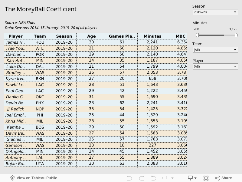
The data here includes all players and all seasons starting at 2014–15 to this current season. You can filter by season, team, minutes, and player. Now that you got threw these 2,000+ words, go enjoy the data and discuss in the comments! I’ll try to answer questions.

Just kidding! Let’s summarize what we just learned today. The MoreyBall Coefficient (MBC) is a metric that measures how efficient a player is when taking into account the positive and negative effects shooting in certain court zones have. Players that are efficient at volume scoring from behind the arc are rewarded positively as well as players who are in general efficient at scoring in general. If a player is a rim-running big, midrange maestro, or just generally inefficient, the metric will be lower than players like James Harden, Damian Lillard, Steph Curry, etc.

To help combat the heavy bias of the three-point shot in the past five or so years, I also developed the MoreyBall Shot Coefficient (MBSC). This metric does not use shots made in it’s calculation, rather just shot attempts. This provides a better understanding if the player has a “MoreyBall” shot profile, i.e. takes most of his shots at the rim, from three, and free throws. If a player doesn’t have a diverse shot profile, their MBSC will not be high. This is why three-point shooters like Duncan Robinson will have a high MBC but a low MBSC. Being an efficient volume three-point shooter will greatly benefit your MBC, but if you are only taking threes, you don’t have a diverse, “MoreyBall” shot profile.

Players that have low MBCs but high MBSCs suggests that the player has a good shot profile but is not efficient. Players with high MBCs and MBSCs suggest that they are both efficient scorers and have a diverse shot profile. Having both a low MSC and a MBSC can mean one of two things: first, the player is inefficient and has a poor or non-diverse shot profile; second, the players may be efficient, but only takes shots in one specific zone. This will primarily be for bigmen like Mitchell Robinson and Clint Capella, so don’t be afraid to use true shooting percentage in conjunction with these stats.

Fin