To the Graduate Council: I am submitting herewith a thesis written by ...

To the Graduate Council:I am submitting herewith a thesis written by Sreenivas Rangan Sukumar entitled“Curvature Variation as Measure of Shape Information.” I have examined the finalelectronic copy of this thesis for form and content and recommend that it be acceptedin partial fulfillment of the requirements for the degree of Master of Science, with amajor in Electrical Engineering.Mongi A. AbidiMajor ProfessorWe have read this thesis andrecommend its acceptance:Michael J. RobertsDavid L. PageAndrei V. GribokAccepted for the Council:Anne MayhewVice Chancellor andDean of Graduate Studies(Original signatures are on file with official student records.)

Curvature Variation as Measureof Shape InformationA ThesisPresented for theMaster of Science DegreeThe University of Tennessee, KnoxvilleSreenivas Rangan SukumarDecember 2004

Acknowledgementsii“Experience is the toughest of teachers, she gives me tests first and lessons later.What I learn is simply information, Experience of information is knowledge.I've learnt that science is organized knowledge, but wisdom is organized life.And most importantly, I have learnt that I definitely have a lot more to learn…!”It was not long ago when I used to think that this section of the document was justanother formality until I realized its significance as a medium to express my gratitude toall the people without whose contribution this work that I am presenting would haveremained a dream.Words are not enough to express what they have done to me. They have given me thelife, the vision and their happiness for my well being and but for their monotonicallyincreasing affection I am sure I would not be what I am today. It is my pleasure todedicate this work to my parents Chellappa Sukumar and Malathi Sukumar.There is an adage that says “You can only take the horse to the pond but cannot make itdrink”. It has been an excellent learning experience under the academic guidance of Dr.Mongi Abidi. He showed me the pond in the Imaging, Robotics and Intelligent SystemsLab and provided me with the right kind of academic, financial and philosophicalsupport all through my pursuit.I shall never forget the quotation on his desk “It is not important what you learn but it isimportant how you teach it to others”. It takes a lot to be an unselfish teacher that youhave been to me. “Thanks a million Dr. Page”. I should thank Dr. Andrei Gribok for thelively discussions of high technical impact on this work. I would like to take thisopportunity to appreciate the efforts of Dr. Andreas Koschan and Dr. Besma Abidiwhose rigorous review and feedback has added to my learning experience in the lab. Dr.Roberts has helped me with the documentation and review of my work. It is not fair if Ido not mention the efforts of Tak Motoyama in the data acquisition process.A significant amount of the learning process at the graduate level has to be attributed tomy peers at the lab. Faysal, Brad and Yohan have been my inspirations towards a PhDdegree and the weekly brainstorming sessions with them have been a good platform tolaunch new ideas. I would like to extend a sincere thanks to Umayal for bequeathing herexperience with the IVP Ranger to me and I shall never forget our evenings at the“Motor pool” scanning under vehicle range data. It’s my pleasure to acknowledgeAshwin, Madhan, Sampath, and Rishi with whom I share “the” cherishable moments atKnoxville.Sincere thanks to you all…

iiiAbstractIn this thesis, we present the Curvature Variation Measure (CVM) as ourinformational approach to shape description. We base our algorithm on shapecurvature, and extract shape information as the entropic measure of the curvature. Wepresent definitions to estimate curvature for both discrete 2D curves and 3D surfacesand then formulate our theory of shape information from these definitions.With focus on reverse engineering and under vehicle inspection, we document ourresearch efforts in constructing a scanning mechanism to model real world objects. Weuse a laser-based range sensor for the data collection and discuss view-fusion andintegration to model real world objects as triangle meshes. With the triangle mesh asthe digitized representation of the object, we segment the mesh into smooth surfacepatches based on the curvedness of the surface. We perform region-growing to obtainthe patch adjacency and apply the definition of our CVM as a descriptor of surfacecomplexity on each of these patches. We output the real world object as a graphnetwork of patches with our CVM at the nodes describing the patch complexity. Wedemonstrate this algorithm with results on automotive components.

Contents1 INTRODUCTION.......................................................................11.1 Motivation ............................................................................................................. 21.2 Proposed Approach ............................................................................................... 41.3 Document Organization......................................................................................... 62 LITERATURE REVIEW...........................................................72.1 Cognition and Computer Vision............................................................................ 72.2 Shape Analysis on 2D Images............................................................................... 82.2.1 Classification of Methods....................................................................................82.2.2 Contour-Based Description ...............................................................................102.2.3 Region-Based Description.................................................................................132.3 Shape Analysis on 3D Models ............................................................................ 162.3.1 Classification of Methods..................................................................................162.3.2 Feature Extraction .............................................................................................172.3.3 Descriptive Representation................................................................................192.3.4 Shape Histograms..............................................................................................202.3.5 Topology Description........................................................................................212.4 Summary ............................................................................................................. 233 DATA COLLECTION AND MODELING ............................263.1 Range Data Acquisition....................................................................................... 263.1.1 Range Acquisition Systems...............................................................................263.1.2 Range Sensing Using the IVP Range Scanner ..................................................273.2 Solid Modeling from Range Images.................................................................... 333.2.1 Modeling Automotive Components for Reverse Engineering...........................333.2.2 Modeling Automotive Scenes for Under Vehicle Inspection............................364 ALGORITHM OVERVIEW ...................................................394.1 Algorithm Description......................................................................................... 394.1.1 Informational Approach to Shape Description – Curvature Variation Measure404.1.2 Curvature-Based Automotive Component Description.....................................414.2 Building Blocks of the CVM algorithm .............................................................. 434.2.1 Differential Geometry of Curves and Surfaces .................................................434.2.2 Curvature Estimation.........................................................................................454.2.3 Density Estimation ............................................................................................484.2.4 Information Measure .........................................................................................565 ANALYSIS AND RESULTS....................................................595.1 Implementation Decisions on the Building Blocks ............................................. 595.1.1 Analysis of Curvature Estimation Methods.......................................................595.1.2 Density Estimation for Information Measure....................................................635.2 State-of-the-Art Shape Descriptors ..................................................................... 665.3 Results of our Informational Approach............................................................... 705.3.1 Intensity and Range Images...............................................................................705.3.2 Surface Ruggedness ..........................................................................................705.3.3 3D Mesh Models ...............................................................................................726 CONCLUSIONS........................................................................816.1 Contributions....................................................................................................... 81iv

v6.2 Directions for the Future ..................................................................................... 826.3 Closing Remarks ................................................................................................. 83BIBLIOGRAPHY.............................................................................84VITA ................................................................................................100

List of TablesviTable 2.1:Qualitative comparison of 3D shape analysis methods with focus onalgorithm efficiency...................................................................................................... 24Table 2.2: Qualitative comparison of 3D shape analysis methods with focus oneffective description. .................................................................................................... 25Table 4.1: Kernel functions. ................................................................................................ 52Table 4.2: List of entropy type measures of the form = == ⋅ϕ................ 57 ⋅ ϕ

viiList of FiguresFigure 1.1: Engineering and reverse engineering ..........................................................2Figure 1.2: Under vehicle inspection and surveillance ..................................................3Figure 1.3: Proposed approach ... ..................................................................................5Figure 2.1: Classification of shape description and representation adapted from[Zhang, 2004] ........................................................................................................9Figure 2.2: [Reproduced from Belongie, 2003] Shape Contexts ................................11Figure 2.3: Classification of methods on 3D data .......................................................17Figure 3.1: IVP Ranger SC-386 range acquisition system..........................................28Figure 3.2: Triangulation and range image acquisition ..............................................30Figure 3.3: The process of calibration ........................................................................32Figure 3.4: Graphical User Interface ..........................................................................33Figure 3.5: Block diagram of a laser-based reverse engineering system ...................34Figure 3.6: Model creation .........................................................................................35Figure 3.7: Data acquisition for under vehicle inspection ..........................................38Figure 4.1: A circle and an arbitrary object .................................................................40Figure 4.2: Block diagram of our CVM as the informational approach to shapedescription ...........................................................................................................41Figure 4.3: Block diagram of curvature-based vehicle component descriptionalgorithm including path decomposition and CVM computation .......................42Figure 4.4: Illustration to understand curvature of a surface .......................................44Figure 4.5: Illustration that shows the effect of bin width on density estimation using ahistogram .............................................................................................................49Figure 4.6: Different methods used to estimate the density of the same dataset.Reprinted from [Silverman, 1986] .......................................................................51Figure 4.7: Effect of bandwidth parameter on kernel density .....................................53Figure 4.8: Resolution issue with Shannon type measures .........................................58Figure 5.1: Neighborhood of a vertex in a triangle mesh ............................................60

viiiFigure 5.2: Curvature analysis – Multi-resolution error analysis experiment withfour different approaches to curvature estimation on triangle meshes ................62Figure 5.3: Curvature analysis – Error in curvature of a sphere at multiple resolutions..............................................................................................................................64Figure 5.4: Curvature analysis – Variation in curvature for surface description ........65Figure 5.5: Curvature-based descriptors.......................................................................67Figure 5.6: Implementation of Shape Distributions ....................................................68Figure 5.7: Shape Distributions and its uniqueness in description ..............................69Figure 5.8: Shape complexity measure– using Shannon’s definition of information .71Figure 5.9: Shape information and surface ruggedness ...............................................72Figure 5.10: Shape information divergence from the sphere – Experimental results onsuper quadrics .......................................................................................................73Figure 5.11: Surface description results - surface, curvature and density of curvature of(a) Spherical cap (b) Saddle (c) Monkey saddle ..................................................75Figure 5.12: Multi resolution experiment on the monkey saddle – The surface, itscurvature density and the measure of shape information ....................................76Figure 5.13: CVM graph results on simple mesh models: curvedness-based edgedetection, smooth patch decomposition and graph representation.......................78Figure 5.14: CVM graph results on automotive parts: curvedness-based edgedetection, smooth patch decomposition and graph representation ......................79Figure 5.15: CVM graph results on an under vehicle scene ........................................80

Chapter 1: Introduction 11 INTRODUCTIONHave we ever realized how easy it has been for us to locate a friend at the shoppingcenter? How quickly we recollect something by looking at a photograph, and howaccurately we approximate distance? It is indeed amazing to realize the design of 126million receptors compactly packed into nerve endings and muscles that coordinate soimpeccably well to process visual information that would require a bandwidth of 600terahertz and processing capability of 2 terabytes per second. We are just measuring thesensing capability of the eye; not to forget the extremely fast and meticulous brain thatdoes the processing at that bandwidth and with incredible accuracy and precision.As computer vision researchers, we acknowledge the uncanny ability of our humanvisual system in object detection and recognition, to address the complexities involvedin imparting this intelligence to a computer. The first and foremost computationalhurdle is that of variability. A vision system needs to generalize across huge variationsof an object to viewpoint, illumination, occlusions and many such factors and still bevery specific. For more than two decades researchers have been fighting such factorsand the lack of important depth information with intensity images. With increase incomputational speed and capabilities of the electronic world, we now deal with 3D data.The 3D sensors, in addition to having the capabilities of traditional cameras, requireprocessing resources to extract depth information. By 3D data, we mean digitizedrepresentations of the real world objects that we can visualize and understand using acomputer. Computers can be programmed to understand a specific domain of objects byextracting features from their digital representation. An important feature used for imageunderstanding is shape. Shape is interpreted as the geometric description of an object,and shape analysis refers to the process of feature extraction followed by featurematching. In this thesis we present the pipeline for 3D data collection and discuss a newshape analysis algorithm that we have developed. We base our algorithm on a featurethat we define as the Curvature Variation Measure (CVM). We have implemented thealgorithm in an application to reverse engineering and vehicle inspection that weelaborate in Section 1.1.

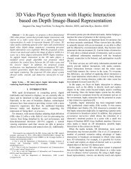
Chapter 1: Introduction 21.1 MotivationComputer aided design (CAD) combined with computer aided manufacturing (CAM)has revolutionized many engineering disciplines since the 1980’s. In particular, CADand CAM technologies have catered to the needs of the automobile manufacturers. Adesigner can now rapidly fabricate a real-world tangible object from a conceptual CADdescription. The process of designing and manufacturing components using a computeris often referred to as computer aided engineering. In this context, we would like tointroduce the idea of reverse engineering that begins with the product and works throughthe design process in the opposite direction to arrive at a product definition statement. Indoing so, it uncovers as much information as possible about the design ideas that wereused to produce that particular product. By design ideas, we mean the shape andtopology of the surfaces used at the time of modeling. At this point, we would like toemphasize that our focus is only on the geometric aspect of reverse engineering and noton the functional aspect of these mechanical components.Reverse engineering aids the electronic dissemination and archival of information inaddition to the prospect of re-creating an out-of-production component. More recently,reverse engineering techniques play a significant role in real-time rapid inspection andvalidation in the production line. The traditional approach to reverse engineering hasbeen the use of coordinate measuring machines (CMM) that require a probe in contactwith the object at the time of digitization. Though CMMs are accurate some applicationsdemand non-contact digitization.In Figure 1.1 we illustrate the process of reverse engineering as the reversal of CAM.We show that the reverse engineering of the disc brake involves acquiring 3D positiondata in the point cloud. We then represent geometry of the object in terms of surfacepoints and tessellated piecewise smooth surfaces. We now need to represent the pointcloud in a form that the CAM system can interpret and manufacture.EngineeringReverse EngineeringFigure 1.1: Engineering and reverse engineering.

Chapter 1: Introduction 3Another application that our research efforts target is that of under vehicle inspection.Vehicle inspection has been traditionally accomplished through security personnelwalking around a vehicle with a mirror at the end of a stick. The inspection personnelare able to view underneath a vehicle to identify weapons, bombs and other securitythreats. The mirror-on-the-stick system allows only partial coverage under a vehicle andis restricted by ambient lighting. The inspecting personnel are also at risk. As part of theSecurity Automation and Future Electromotive Robotics (SAFER) program we aim atdeveloping a robotic platform that deploys “sixth sense” sensors for threat assessment.We propose the idea of incorporating a 3D range sensor on the robotic platform. Theidea is to be able to extract the 3D geometry of the undercarriage of automobiles. Withprior manufacturer’s information on the components that make the undercarriage of thevehicle, we believe that it will be possible to identify foreign objects in the scene. Forexample in Figure 1.2 we show the robotic platform and the 3D geometry of the scenecontaining the muffler, shaft and the catalytic converter. It will not be possible to extractcomplete geometry of the undercarriage without dismantling the automobile. We henceneed a representation scheme that maps the shape sensed from the scene to the CADdescription and that is robust with occluded data.Though vehicle inspection and reverse engineering appear as different applications,they share the same processing pipeline as a computer vision task of designing asystem that can capture the geometric structure of an object and store the subsequentshape and topology information. We discuss the use of laser-based range scanners forthe extraction of 3D geometry and a curvature-based shape analysis algorithm basedon our CVM to interpret surface topology.Robotic Platform Under Vehicle Scene 3D GeometryFigure 1.2: Under vehicle inspection and surveillance.

Chapter 1: Introduction 41.2 Proposed ApproachShape analysis is an age-old research topic and has been pursued since the dawn ofimage processing and computer vision. Literature on shape extraction from intensityimages is vast and gives good insight into why vision research with intensity imageshas not been very successful. Most of the methods we have studied show promise withmore and almost complete information with 3D data. Though 3D data acquisition andprocessing is relatively new, there are a few important contributions in our context ofshape similarity and shape description all motivated by the challenge of objectrecognition. We survey the literature on shape analysis applied to intensity images andalso summarize recent and ongoing work in 3D computer vision.Computer vision systems seek to develop computer models of the real world throughprocessing of image data from sensors. In Figure 1.3(a) we present the flow diagramof our proposed approach. We begin with the data acquisition (Figure 1.3 (b)) usinglaser-based range scanners and the process of creating CAD models using thesescanners. We acquire range images using the laser-illuminated active range sensorfrom the Integrated Vision Products Inc. (IVP). A range image is a 2D matrix withvalues proportional to the distance between the sensor and the object. We acquirerange information from multiple views of the object to make sure that we havesufficient data to represent the object completely. We then transform the range datafrom the camera coordinate frame to the real world and integrate the multi-view pointclouds into a single global reference frame. We reconstruct triangle meshes from thepoint clouds and use it as our input for the shape analysis.We base our shape analysis algorithm on the part-based perception model[Stankiewicz, 2002]. With automotive components, our task is simplified because thecomponents are man-made and manufacturing limitations restrict us to smooth (mostlyplanar and cylindrical) patches. We hence propose that surface shape description ofeach of the parts and the connectivity of parts can uniquely describe the object. Indescribing surfaces and surface complexity we chose curvature to extract “shapeinformation”. We chose curvature because it is an information preserving feature,invariant to rotation and possesses an intuitively pleasing correspondence to theperceptive property of “simplicity”. We decompose the object of interest into a set ofpatches and assign a Curvature Variation Measure (CVM) to each of these patches andrepresent the object as a patch adjacency graph. Our graph representation whenextended to scenes with occlusions can still yield satisfactory results.Consider the example in Figure 1.3 again. We first decompose the triangle meshmodel into smooth patches. We show the disc brake model and decompose it into fourparts. We have shaded each of these parts with a different color. We base our surfacepatch decomposition on the definition of curvedness in [Dorai, 1996]. Curvednessidentifies sharp edges and creases.

Chapter 1: Introduction 5Real WorldObjectData Acquisitionand ModelingSurface PatchDecompositionCurvatureVariation MeasureGraphRepresentation0.01 0.110.11 0.001(a)Multi-ViewRange ImagesMulti-ViewRegistrationViewIntegrationMeshModelingComputeCurvedness(b)Segment byRegion GrowingConnectivity ofSurface Patches(c)CurvatureComputationDensityEstimationInformationMeasureCVM = 0.001(d)Figure 1.3: Proposed approach. (a) Shape analysis based on our curvature variationmeasure - flow diagram. (b) Data acquisition and modeling. (c) Surface patchdecomposition. (d) Curvature variation measure.

Chapter 1: Introduction 6We then perform region-growing segmentation and save the patch adjacencyinformation as illustrated in Figure 1.3(c).Now that we have segmented surface patches that make the object, we compute thecurvature variation measure on each of these patches (Figure 1.3(d)). We haveborrowed concepts from Shannon’s idea [Shannon, 1948] of measuring information ona probabilistic framework. We hence define the curvature variation measure as theentropy of curvature along that surface. We present a brief analysis on variouscurvature estimation methods on triangle meshes and reiterate the importance ofbandwidth optimized density estimation to stabilize the information measure. Ourmodification of Shannon’s definition of entropy is normalized and invariant to scale.The normalized resolution invariant measure attempts to quantify the complexity ofthe surface by a single number. Similar shapes at different scales will have equalmeasures.1.3 Document OrganizationThe remainder of this thesis documents the theory and results of our data collectionand CVM algorithm. Chapter 2 presents a survey of the literature on the shape analysisand description of 2D images and 3D models. Here we explain why methods in 2Dcannot be extended to 3D and discuss the scope for extending the state of the art.Then, we present our experience with the data acquisition using a laser-based scannerfor creating 3D models of automotive components and scenes under the vehicle inChapter 3. Chapter 4 documents the theory that supports our shape analysis algorithm.We test our algorithm on the acquired data and present our results in Chapter 5. Theseexperimental results demonstrate capabilities of our algorithm and its scope as anobject recognition system. Finally, we conclude with possible extensions in Chapter 6.

Chapter 2: Literature Review 72 LITERATURE REVIEWIn this chapter we present a review of the research literature. In Section 2.1 weintroduce the reader to shape and its implication to computer vision and briefly reviewsome key methods on 2D images in Section 2.2. We discuss contemporary research in3D computer vision for shape analysis in Section 2.3 and summarize our survey inSection 2.4.2.1 Cognition and Computer VisionThe human cognitive system is designed to interpret sensory data with suchremarkable speed and accuracy that we fail to appreciate millions of computationsinvolved in a common event of identifying an object. An impressive component inhuman perception is our ability to recognize 3D objects from their 2D retinalprojections. Stankiewicz outlines human visual perception into three possiblehypotheses, namely the feature model approach, alignment model approach and thepart-based approach [Stankiewicz, 2002]. Feature models propose that the visualsystem does not match a precise numerical array of an object with another butremembers a collection of features in memory. According to this approach the locationof the features in a particular image is less significant than its presence in the image.The feature model approach fails with increasing occlusions and is less reliable whenthe spatial relationship between the features and the image are vital in recognizing theobject. Alignment models make use of the spatial information to compensate forviewpoint changes but do not consider occlusions. They can handle Euclideantransformations such as the rotation, translation and scaling and are accepted to berobust in comparison with the feature models. Part-based models operate bydecomposing an object into its constituent parts. The approach uses image features todescribe the shape of parts in addition to documenting relationships between parts.The part-based model has not met with great success in computer vision because ofthe insufficiency in intensity images to segment objects as parts, but with theincreasing computational capabilities and improvements in sensor technology towards3D imaging, part-based models are a good prospect.

Chapter 2: Literature Review 8Shape is the geometric information invariant to a particular class of transformationssuch as affine, translation, rotation and scaling and is considered to be the “words” ofthe visual language. Shape analysis is an important aspect in image understanding.Since so many objects in our world are strongly determined by geometric properties,the applications of shape analysis extend over a broad spectrum of science andtechnology. Indeed, when properly and carefully applied shape analysis provides richpotential for applications in diverse areas, spanning computer vision, graphics,material sciences, biology and even neuroscience.2.2 Shape Analysis on 2D ImagesShape description looks for effective and perceptually important shape features basedon either shape boundary information or interior content. By perceptually similarshapes we are referring to shapes that are rotated, translated, scaled and are affinetransformed. Many shape representation techniques have been developed in the pastand shape analysis still remains as an interesting field of research. A few suchrepresentation techniques are the shape signatures, shape histograms, moments,curvature, shape context and shape matrix. We would like to direct the reader to[Zhang and Lu, 2004] for a recent and comprehensive survey on 2D shaperepresentation for various applications.2.2.1 Classification of MethodsShape representation techniques are generally classified into two classes based onwhether shape features are extracted from the contour only or from the whole region.Zhang and Lu [Zhang and Lu, 2004] subdivide each of these classes further intostructural and global approaches based on the primitives used to describe the shape.They discuss methods that operate on the space domain and transform domain toextract shape information and classify shape description methods as shown in Figure2.1.Contour-based approaches are more popular in computer vision literature. Suchmethods assume that human beings discriminate shapes mainly by their featurecontours. The contour-based approach is limited by noise and by data that do not havesufficient information (occlusions) in the boundary contour. Region-based methodsare considered to be more robust and are dependable for accurate retrieval as theyattempt to extract shape information from the entire region and not just its boundary.

Chapter 2: Literature Review 92D ShapeContour-basedRegion-basedStructural Global Global StructuralChain CodePolygonB-SplineInvariantsPerimeterCompactnessEccentricityShape SignatureHausdorff DistanceWaveletsScale SpaceAutoregressiveElastic MatchingAreaEuler NumberEccentricityGeometricMomentsZernike momentsFourierDescriptorGrid MethodShape MatrixConvex HullMedial AxisCoreFigure 2.1: Classification of shape description and representation adapted from[Zhang, 2004].

Chapter 2: Literature Review 102.2.2 Contour-Based DescriptionContour-based shape representation techniques extract shape information from theboundary. There are generally two approaches for contour shape modeling: thecontinuous global approach and discrete structural approach. The global approachmakes use of feature vectors derived from the boundary to describe shape. Themeasure of shape similarity is the metric distance between feature vectors. Thediscrete approach to shape analysis represents the shape into a graph or tree ofsegments (primitives). The shape similarity is deduced by string or graph matching.We begin our analysis with the contour-based global shape description methods. Themost commonly used global shape descriptors are surface area, circularity,eccentricity, convexity, bending energy, ratio of principle axis, circular variance andelliptic variance and orientation. These simple descriptors are not suitable standalonedescriptors but are usually used to discriminate shapes with large differences or tofilter false hits. Some of these are also used in combination with the other descriptorsfor shape description. The efficiency of such descriptors is discussed in [Peura andIvarinen, 1997].A few space-domain techniques compute correspondence-based shape measures usingthe point-point match where each point on the boundary is considered to be acontributor to shape. Hausdorff distance is a classical correspondence-based shapematching method, often used to locate objects in an image and measure similaritybetween shapes as discussed in [Huttenlocher, 1992].Given two shapes S 1 = {a 1 , a 2 ,,……. ,a p } and S 2 = {b 1 , b 2 ,,……. ,b p } represented astwo sets of points, the Hausdorff distance is defined asHd(S1,S2) = max(h(S1,S2),h(S2,S1)}, h(S1,S2) = max min|| a − b ||a∈ S1 b∈S 2(2.1)where ||.|| refers to the Euclidean distance.The Hausdorff distance measure is too sensitive to noise and is useful for partialmatching invariant to rotation, scale and translation. Rucklidge improves it with a newmeasure between two datasets using a prohibitively expensive matching procedurethat tackles different orientations, positions and scales [Rucklidge, 1997]. A morerecent but similar kind of approach to shape matching was introduced by the name of“shape contexts” in [Belongie et al., 2002].Shape contexts claim to extract globalfeature at every point reducing the point-point matching into a matrix matching ofcontexts. To extract the shape context at a point p on the boundary, the vectors thatconnect p and each of the other points on the boundary are computed. The length andorientation of these vectors are quantized into a log-space histogram map for that pointp to account for additional sensitivity to neighboring points. These histograms areflattened and concatenated to form the context of the shape as shown in Figure 2.2.

Chapter 2: Literature Review 11(a) (b) (c) (d) (e)Figure 2.2: [Reproduced from Belongie, 2003] Shape Contexts. (a) A charactershape. (b) Edge image of (a). (c) The histogram is the context of the point p. (d) Thelog-space histogram. (e) Each row of the context map is the flattened histogram ofeach point context, the number of rows is the number of sampled points.Davies [Davies, 1997] describes shape signatures as a one-dimensional functionderived from the shape boundary points. Some shape signatures that can be found inthe literature are the centroidal profile, complex coordinates, tangent angle, cumulativeangle, chord length and curvature. Shape signatures are usually normalized in scale.Translational and rotational invariance is achieved by a shift search procedure of theone dimensional function extracted from the shape boundary. Shape signatures requirefurther processing in addition to the high matching cost to overcome their sensitivityand improve robustness. Autoregressive models [Chellappa and Bagdazian, 1984] arestochastically defined predictor-based methods dependent on modeling the shape intoa 1D function.Boundary moments are extensions of shape signatures to reduce the dimensionality ofthe boundary representation. If z(i) is an extracted shape signature of a boundary, ther th moment and the central moment µcan be estimated as shown in Equation 2.2 and2.3.rm1µ =1Nrr= [ z( i )]N i=1N[ z( ir) − m1]N i=1(2.2)(2.3)where N is the number of points representing the boundary. The normalized momentsare invariant to shape translation, rotation and scaling. As discussed in [Gonzalez,2002] the amplitude of the shape signature can be treated as a random variable and itsmoments computed using its histogram. These moments are easily computable buthave no physical significance.

Chapter 2: Literature Review 12Bimbo [Bimbo, 1997] implements elastic matching for shape-based image retrieval. Adeformed template is generated as the sum of the original template and a warpingdeformation. The similarity between the original shape of the template and the objectis obtained by minimizing the compound function, which is the sum of the strainenergy, bending energy and the deviation measure of the deformed template with theobject. He defines shape complexity as the number of curvature zero crossings and acorrelation between curvature functions of the template and the object. Theclassification is performed by a back propagation algorithm neural network.Most of the space-domain techniques discussed in literature are sensitive to noise andboundary deviations. Spectral-domain techniques resolve the noise issues. Thesimplest of the spectral domain descriptors are the Fourier descriptors [Zhang and Lu,2002] and the wavelet descriptors [Yang et al., 1998]. They are derived from the onedimensionalshape signatures of the shape function. They are easy to compute,normalize and bypass the complex matching stages of the shape signature basedmethods. Zhang and Lu [Zhang and Lu, 2002] argue that the centroidal profile is themost efficient shape descriptor to be used in combination with Fourier descriptors.Structural shape representation is yet another approach to analysis of shape descriptionas shown in Figure 2.1. With the structural approach, shapes are broken down intosegments called shape primitives. Structural methods differ in the selection ofprimitives and organization of primitives for shape representation. Some of thecommon methods of boundary decomposition are based on polygonal approximation,curvature decomposition and curve fitting. The result of the decomposition is encodedin a general string form that can be used with a high-level syntactic analyzer for shapecomparison tasks.Chain code described by [Freeman and Saghri, 1978] is a sequence of unit-size linesegments with a given orientation. The unit vector method describes any arbitrarycurve as a sequence of small vectors of unit length in a set of directions. The chaincodes need to be independent of the starting boundary pixel. The independence isachieved by a good scheme that defines the characteristics of a starting pixel or byrepresenting the chain code as differences in successive directions. Chain codes usedfor object recognition and matching are not scale invariant though they are rotationinvariant. Polygonal decomposition methods discussed in [Groskey et al., 1992] breaka given boundary into line segments by using polygon vertices as primitives. Featurestrings are created with four elements such as the internal angle, distance from the nextvertex and the coordinates of the vertex. The similarity of shapes is the editingdistance between two feature strings representing the shape. Mehrotra and Gary in[Mehrotra and Gary, 1995] represent shape as a series of interest points from thepolygonal boundary approximation. These points are mapped onto a new scale androtation invariant basis to represent shape in a new coordinate system. Berretti et al.[Berretti et al., 2000] extend [Groskey and Mehrotra, 1990] for shape retrieval by

Chapter 2: Literature Review 13defining tokens as the zero crossings of Gaussian curvature and shape similarity is theEuclidean distance between primitives. Dudek and Tsotsos [Dudek and Tsotsos, 1997]use curvature scale spaces for shape matching. In this approach, shape primitives arefirst obtained from a curvature-tuned smoothing technique. A segment descriptorconsists of the segment’s length, ordinal position, and curvature turning valueextracted from each of these primitives. A string of segment descriptors is then createdto describe the shape. For two shapes A and B represented by their string descriptors, amodel-by-model match using dynamic programming is exploited to obtain thesimilarity score of the two shapes. To increase robustness and to save matchingcomputation, the shape features are put into a curvature scale space so that shapes canbe matched even in different scales. However, due to the inclusion of length in thesegment descriptors, the descriptors are not scale invariant.Another interesting approach to the analysis of shape is syntactic analysis in [Fu,1974] that attempts to simulate the structural and hierarchical nature of the humanvision system. In syntactic methods, shape is represented by a set of predefinedprimitives. The set of predefined primitives is called the codebook and the primitivesare called code words. The matching between shapes can use string matching byfinding the minimal number of edit operations in trying to convert one string toanother However, it is not practical in general applications due to the fact that it is notpossible to infer a pattern of grammar which can generate only the valid patterns. Inaddition, this method needs a priori knowledge for the database in order to definecodeword or alphabets. Shape invariants make use of simple shape descriptors such asthe cross ratio, length and area to derive a multi-valued signature. Kliot and Rivlin[Kliot and Rivlin, 1998] propose a multi valued matrix that can be used for matchingtwo curves. This method can be improved with a histogram matching stage before thematrix matching. Squire and Caelli in [Squire and Caelli, 2000] use the densityfunction of piecewise linear curves for their shape invariant. The histogram of theshape invariant signature is fed into a neural network for classification.2.2.3 Region-Based DescriptionRegion-based techniques take into account all the pixels within a shape region toobtain the shape representation, rather than only use boundary information as incontour-based methods. Common region-based methods use moment descriptors todescribe shapes. Structural methods include grid method, shape matrix, convex hulland medial axis. Global methods treat shape as a whole; the resultant representation isa numeric feature vector which can be used for shape description while structuralmethods break down the shape into segments. Similarity between global shapedescriptors is simply the metric distance between their feature vectors. Some of theglobal descriptors are the geometric moment invariants and the algebraic momentinvariants. One of the oldest global methods implemented for region-based description

Chapter 2: Literature Review 14is from Hu [Hu, 1962]. He used the work of nineteenth century mathematicians onimages for pattern recognition.p qmpq = x y f ( x, y ), p,q = 0 , 1,2....x y(2.4)Lower-order geometric moments from Equation 2.4 are easy to compute and aresufficient for representing simple shapes. Algebraic moments [Taubin and Cooper,1991] and [Taubin and Cooper, 1992] on the other hand are based on the centralmoments of predetermined matrices that can be constructed for any order and areinvariant to affine transformations. Teague [Teague, 1980] defines orthogonalmoments by replacing the x p y q term by the Zernike polynomials. Moment shapedescriptors are concise, robust, and easy to compute and match. The disadvantage ofmoment methods is that it is difficult to correlate higher-order moments with theshape’s physical features.Among the many moment shape descriptors, Zernike moments [Jeannin, 2000] are themost desirable for shape description. Due to the incorporation of a sinusoid functioninto the kernel, they have similar properties of spectral features, which are wellunderstood. Although Zernike moment descriptors have a robust performance, theyhave several shortcomings. First, the kernel of Zernike moments is complex tocompute, and the shape has to be normalized into a unit disk before deriving themoment features. Second, the radial features and circular features captured by Zernikemoments are not consistent, one is in the spatial domain and the other is in spectraldomain. This approach does not allow multi-resolution analysis of a shape in the radialdirection. Third, the circular spectral features are not captured evenly at each other andcan result in loss of significant features which are useful for shape description.To overcome these shortcomings, a generic Fourier descriptor (GFD) has beenproposed by Zhang and Lu [Zhang and Lu, 2002]. The GFD is acquired by applying a2D Fourier transform on a polar-raster sampled image using the Equation 2.5.PF ( ρ,φ ) =2 r 2πif ( r, θi)expj2π( ρ + ϕ Rr i T(2.5)Zhang and Lu show that GFD outperforms contour shape descriptors such as curvaturescale spaces, Fourier descriptors and moment-based descriptors.The grid shape descriptor proposed by [Lu and Sajjanhar, 1999] has been used in[Chakrabarti et al., 2000] and [Safar et al., 2000]. Basically, a grid of cells is overlaidon a shape; the grid is then scanned from left to right and top to bottom. The result issaved as a bitmap. The cells covered by the shape are assigned one and those notcovered by the shape are assigned zero. The shape can then be represented as a binary

Chapter 2: Literature Review 15feature vector. The binary Hamming distance is used to measure the similaritybetween two shapes. To account for the invariance to Euclidean transformations theshape needs to be normalized. Chakrabarti et al. [Chakrabarti et al., 2000] improve thegrid descriptor by using an adaptive resolution (AR) representation acquired byapplying quad-tree decomposition on the bitmap representation of the shape.Typically, shape methods use rectangular-grid sampling to acquire shape information.The shape representation so derived is usually not translation, rotation and scalinginvariant. Extra normalization is therefore required. Goshtasby [Goshtasby, 1985]proposes the use of a shape matrix which is derived from a circular raster samplingtechnique. The idea is similar to normal raster sampling. However, rather than overlaythe normal square grid on a shape image, a polar raster of concentric circles and radiallines is overlaid in the center of the mass. The binary value of the shape is sampled atthe intersections of the circles and radial lines. The shape matrix is formed such thatthe circles correspond to the matrix columns and the radial lines correspond to thematrix rows. Prior to the sampling, the shape is scale normalized using the maximumradius of the shape. The resultant matrix representation is invariant to translation,rotation, and scaling. Since the sampling density is not constant with the polarsampling raster, Taza et al. represent shape using a weighed shape matrix, which givesmore weight to peripheral samples in [Taza et al., 1989]. However, since a shapematrix is a sparse sampling of shape, it is easily affected by noise. Besides, shapematching using a shape matrix is expensive. Parui et al. propose a shape descriptionbased on the relative areas of the shape contained in concentric rings located in theshape center of the mass in [Parui et al., 1986].Structural methods for region-based shape description usually involve the convexhulls and medial axis described in [Davies,1997], [Blum,1967] and [Morse,1994]. Aregion R is convex if and only if for any two points x 1 ; x 2 R, the whole linesegment x 1 x 2 is inside the region. The convex hull of a region is the smallest convexregion H which satisfies the condition R H. The difference H − R is called theconvex deficiency D of the region R. The extraction of the convex hull can beachieved either using the boundary-tracing method from [Sonka et al., 1993] or byusing morphological methods from [Gonzalez and Woods, 1992]. Since shapeboundaries tend to be irregular because of digitization noise and variations insegmentation result in a convex deficiency that has small, meaningless componentsscattered throughout the boundary. Common practice is to first smooth a boundaryprior to partitioning. The polygon approximation is particularly attractive because itcan reduce the computation time taken for extracting the convex hull from O (n 2 ) to O(n) (n being the number of points in the shape). The extraction of convex hull can be asingle process which finds significant convex deficiencies along the boundary. Afuller representation of the shape is obtained by a recursive process which results in aconcavity tree. Here the convex hull of an object is first obtained with its convexdeficiencies, then the convex hulls and deficiencies of the convex deficiencies are

Chapter 2: Literature Review 16found, and the recursion follows until all the derived convex deficiencies are convex.The shape can then be represented by a string of concavities (concavity tree). Eachconcavity can be described by its area, bridge (the line that connects the cut of theconcavity) length, maximum curvature, distance from maximum curvature point to thebridge. The matching between shapes becomes a string or a graph matching.Like the convex hull, a region skeleton is also employed for shape representation. Askeleton may be defined as a connected set of medial lines along the limbs. The basicidea of the skeleton is to eliminate redundant information while retaining only thetopological information concerning the structure of the object that can help withrecognition. The skeleton methods are represented by Blum’s medial axis transform(MAT) [Blum, 1967]. The medial axis is the locus of centers of maximal disks that fitwithin the shape. The bold line in the figure is the skeleton of the shaded rectangularshape. The skeleton can then be decomposed into segments and represented as a graphaccording to a certain criteria. The matching between shapes becomes a graphmatching. The computation of the medial axis is a rather challenging problem. Inaddition, medial axis tends to be very sensitive to boundary noise and variations.Preprocessing the contour of the shape and finding its polygonal approximation hasbeen suggested as a way of overcoming these problems. But, as has been pointed outby Pavlidis [Pavlidis, 1982] obtaining such polygonal approximations can be quitesufficient in itself for shape description. Morse [Morse, 1994] computes the core of ashape from medial axis in scale space.We conclude this section with a note that shape description from intensity images haveto deal with view occlusions and lack of sufficient information. We now study someimportant methods used for shape analysis on 3D mesh models in Section 2.3.2.3 Shape Analysis on 3D ModelsIn Section 2.2, we have reviewed techniques implemented for shape extraction in 2Dintensity images. In the following section we present a classification of methods in theliterature on digitized 3D representations. We follow the classification with a briefdescription of some interesting methods.2.3.1 Classification of MethodsThere is a multitude of techniques to assess the similarity among 2D shapes as discussedin the Section 2.2. Most of the techniques do not extend to 3D models because of thedifficulty of extending parameterization of the boundary curve extracted from 2D to 3D.In simple words, given a 2D shape, its parameterization is a straightforward 1D curve.With a 3D real world object it is difficult because when it is projected onto a 2D imageplane, one dimension of object information is lost. The 3D domain requires dealing with

Chapter 2: Literature Review 17objects of different genus which makes it impossible for most of the 2D similarityassessment methods extendable to 3D. The challenge in 3D computer vision is morethan just the lack of information as in the 2D case and needs to address thecomputational effort and descriptive representation. The 3D data usually are representedas meshes or assemblies of simple primitives. The representation scheme is suitable forvisualization but not for recognition and computer vision tasks. The process of shapeassessment hence becomes a two step process: (1) the shape signature extraction and (2)the comparison of shape signatures with distance functions. Based on how the shape isextracted from the 3D model representation techniques can be classified as shown inFigure 2.3.2.3.2 Feature ExtractionFeature extraction techniques usually attempt to represent the shape of the 3D objectby a combination of one-dimensional feature vectors. A common approach forsimilarity models is based on the paradigm of feature vectors. A feature transformmaps a complex object onto a feature vector in a multidimensional space. Thesimilarity of two objects is then defined as the vicinity of their feature vectors in thefeature space. Geometric parameters and ratios such as the surface area, volume ratio,compactness, Euler numbers and crinkliness have been used with limiteddiscrimination capabilities.3D ShapeFeature ExtractionDescriptiveRepresentationShape HistogramsTopologyDescriptionShape ContextShock GraphsAlpha ShapesAspect GraphSpin ImagesHarmonic Shape ImagesCOSMOSGeometry ImagesShape DistributionsSpider modelLocal Feature HistogramReeb graphSkeletal graphsModel SignaturesFigure 2.3: Classification of methods on 3D data.

Chapter 2: Literature Review 18Kortgen et al. [Kortgen et al., 2003] achieves shape matching by extending the 2Dshape contexts [Belongie, 2003] to 3D. They use the shape context at a point on thesurface as the summary of the global shape characteristics invariant to rotation,translation and scaling. Vranic and Saupe [Vranic and Saupe, 2001] propose a newmethod for shape similarity search on polygonal meshes. They characterize spatialproperties of 3D objects such that similar objects are mapped as close points in thefeature space. They then perform a coarse voxelization of the object in the canonicalcoordinate frame and compute the absolute value of the 3D Fourier coefficients as thefeature vector. Vranic improves it further in [Vranic, 2003]. Ohbuchi et al. [Obhuchi etal., 2003] describe a multi-resolution analysis technique for the task of shapesimilarity comparison. They use 3D alpha shapes to generate a multi-resolutionhierarchy of shapes of a given query object. They then follow that by applying asimple shape descriptor such as the D 2 shape function introduced by [Osada et al.,2002] on each of the multi-resolution representations and call it the multi-resolutionshape descriptor.Automated feature recognition has also been attempted by extracting instances ofmanufactured features from engineering designs. Henderson [Henderson et al., 1993]is an extensive survey of such methods that make use of a library of machiningfeatures for description. With the assumption of primitives, procedural methodsproposed by Elinson et al. [Elinson et al., 1997] and Mukai et al. [Mukai et al., 2002]have applied constructive solid geometry (CSG’s) to classify CAD models ofmechanical parts. Their methods however cannot be extended to a more general classof shapes represented as point sets and meshes. Biermann et al. in [Biermann et al.,2001] propose Boolean operations of primitives for shape description. However, directassessment of similarity between 3D models using Boolean operations iscomputationally slow due to the difficulty in aligning the models before performingthe operation. With a large database, it is not a pragmatic solution. Zhang and Chen[Zhang and Chen, 2001] discuss efficient global feature extraction methods from themesh representation.Duda and Hart [Duda and Hart, 1973] have been extended by Khotanzad et al.[Khotanzad et al., 1980] to a subset of 3D moments that are invariant to rotation,translation and scaling that can be used as feature vectors for shapes as shown inEquation 2.6.∞∞∞ m = x y z ρ (x, y,z) dxdydzpqr−∞ −∞ -∞pqrwhere ρ (x, y, z) represents the point cloud of the model. (2.6)Cybenko et al. [Cybenko et al., 1997] use second-order moments, spherical kernelmoment invariants, bounding-box dimensions, object centroid and surface area alongwith a correlation metric for shape-similarity measurement. Elad et al. [Elad et al.,

Chapter 2: Literature Review 192001] implement support vector machines for adaptively selecting weights fordistance measurements between moments for shape similarity. Corney et al. [Corneyet al., 2002] compute the Euclidean distance between simple geometric ratios for ashape similarity measure. Cyr and Kimia [Cyr and Kimia, 2001] use a shock graphbasedshape similarity metric to assess the similarity between 3D models. Adjacentviews are clustered in, thus generating the aspect using a seeded-region growingtechnique that satisfies the local monotonicity and specific distinctiveness of theaspect view criteria. The comparison of two 3D models is achieved by matching the2D aspect views.2.3.3 Descriptive RepresentationIn this category of methods, shape matching is achieved through an intermediaterepresentation that aides a matching stage. These methods are usually robust but arecomputationally expensive. Usually the 3D information is broken down into a stack of2D descriptors on which robust 2D shape matching techniques can be applied.Dorai presents COSMOS (Curvedness-Orientation-Shape Map on Sphere) [Dorai,1996] as a representation scheme for 3D free form objects from range data withoutocclusions. According to this scheme, the object is represented concisely in terms ofmaximal surface patches of constant shape index. The shape index is a quantitativemeasure of shape complexity of the surface and is based on the principle curvatures ata point on the surface. The patches are mapped onto a sphere based on the orientationsand aggregated using shape spectral functions. Surface area, curvedness andconnectivity are utilized to capture global shape information. She derives a shapespectrum and experiments on its efficiency of recognition.Johnson and Hebert [Johnson and Hebert, 1999] introduce spin images for a 3D shapebasedobject recognition system towards simultaneous recognition of multiple objectsin scenes containing clutter and occlusion. The spin image is a data level descriptorthat is used to match surfaces represented as surface meshes. They describe surfaceshape as a dense collection of points and surface normals and associate a descriptiveimage with each surface point that encodes global properties of the surface using anobject centered coordinate system. The spin image is created by constructing a localbasis at an oriented point on the surface of the object and accumulates geometricparameters in a 2D histogram. In simple words, the spin image can be visualized as asheet spinning about the normal at that point. The image is descriptive because itaccounts for all the points on the surface and is invariant to rigid transformations.Kazhdan et al. [Kazhdan et al., 2003] outline an algorithm for 3D shape matchingusing a harmonic representation of 3D polygonal meshes. They rasterize the 3D meshinto 64 x 64 x 64 voxel grids and center the object as the center of the grids so that the

Chapter 2: Literature Review 20bounding sphere is of radius 32 voxels. They then treat the object as the function in 3Dspace and decompose it into 32 spherical functions by considering spheres of radii 1through 32. They further decompose each of the functions into 16 harmoniccomponents and the 32 x 16 harmonics constitute the harmonic representation of the3D model. They compare two harmonic representations with the Euclidean distance.Zhang and Hebert propose the harmonic shape images as a 2D representation ofsurface patches [Zhang and Hebert, 1999]. The theory of harmonic maps studies themapping between different metric manifolds from the energy minimization point ofview. With the application of harmonic maps, a surface representation called harmonicshape images is generated to represent and match 3D freeform surfaces. The basic ideaof harmonic shape images is to map a 3D surface patch with disc topology to a 2Ddomain and encode the shape information of the surface patch into the 2D image. Thissimplifies the surface-matching problem to a 2D image-matching problem.Shum et al. address the problem of 3D shape similarity between closed surfaces in[Shum et al., 1996]. He defines a shape similarity metric as the L 2 distance betweenthe local curvature distributions over the spherical mesh representations of the twoobjects. He achieves the similarity measure in O (n 2 ) complexity where n is thenumber of tessellations in the object mesh. Their experiments on simple shapes showgood shape similarity measurements.2.3.4 Shape HistogramsThe histogram-based methods reduce the cost of complex matching schemes butsacrifice efficiency and robustness to the methods discussed in Section 2.3.2. Thesemethods compare shapes on the basis of their statistical properties.Ankerst et al. [Ankerst et al., 1999] introduce 3D shape histograms as an intuitivepowerful approach to structural classification of proteins. They decompose a 3Dobject into three models (shell model, sector model and spider web) around an object’scentroid and process model similarity queries based on a filter refinement architecture.A similar search technique for mechanical parts using histograms was proposed in[Kriegel et al., 2003]. The models are normalized into a canonical form and voxelizedinto axis parallel equal partitions. Each of these partitions is assigned to one or severalbins in a histogram depending on the specific similarity model.Besl et al. [Besl et al., 1995] consider histograms of crease angles for all edges in atriangle mesh to describe shape. Their method does not match non-manifold surfacesand is not invariant to changes in mesh tessellation. Osada et al. in [Osada et al., 2002]presents Shape Distributions for a shape similarity search engine by extending Besl’sapproach. According to his technique, random points from the surface of a model are

Chapter 2: Literature Review 21extracted. Shape functions D 1 , D 2 , D 3 , D 4 , and A 3 are computed at each of theserandom points.•D 1 : Distance between a fixed point (centroid) and a random point.•D 2 : Distance between two random points.•D 3 : Square root of the area of triangle formed by three random points.•D 4 : Cube root volume of the tetrahedron of four random points.•A 3 : Angle between three random points.They suggest the use of D 2 shape function for computing Shape Distributions due toits robustness and efficiency along with invariance to rotation and translation. The D 2distances between random points are normalized using the mean distance. The shapedistribution is the histogram that measures the frequency of occurrence of distanceswithin a specified range of distance values. Once the Shape Distributions aregenerated the distance between the two solid shapes is computed using L N norm.Usually L 2 norm is used for comparison, though other distances such as Earth Mover’sdistance or match distances can also be used.This technique is robust and efficient for simple objects and gross shape similarity. Asthe resolution of the 3D model increases the comparison becomes more robust, but thecomputational time increases. Furthermore as objects become more and morecomplex, the Shape Distributions tend to assume similar shape resulting in inaccuratecomparison of solid models. Shape Distributions have been experimented with limitedsuccess on mechanical parts and real laser scanned data. Ohbuchi et al. in [Ohbuchi etal., 2003] improve the performance of Shape Distributions with a 2D histogram ofangle-distance and absolute angle distance that can be computed from the D 2 shapedistribution. Page et al. [Page et al., 2003b] define shape information as the entropy ofthe curvature density. They use it to describe the complexity of the 3D shape. Hetzel etal. [Hetzel et al., 2001] present an occlusion robust algorithm for 3D objectrecognition that makes use of local features such as the shape index, pixel depth andthe surface normal characteristics in a multidimensional histogram. Histograms of twoobjects are matched and verified using the chi–squared hypothesis test to achieveshape recognition.2.3.5 Topology DescriptionThe topology of a 3D model is an important property for measuring similarity betweendifferent models. Topology of models is typically represented in the form of arelational data structure such as trees or directed acyclic graphs. Subsequently, thesimilarity estimation problem is reduced to a graph or tree comparison problem.

Chapter 2: Literature Review 22Gotsman et al. describe the fundamentals of spherical parameterization for 3D meshes[Gotsman et al., 2003]. They argue that closed manifold genus-zero meshes aretopologically equivalent to a sphere and assign a 3D position on the unit sphere toeach of the mesh vertices. They use barycentric coordinates for the planarparameterization. Leibowitz et al. [Leibowitz et al., 1999] share their memoryintensive experience in implementing geometric hashing for the comparison of proteinmolecules represented as 3D atomic structures.In [McWherter et al., 2001] model signature graphs have been proposed fortopological comparison of solid models. They extend attribute adjacency graphs,mentioned in [Joshi and Chang, 1998], to consider curved surfaces. Model signaturegraphs are constructed from boundary representation of the solid. This graph forms theshape signature of the solid model. Once a model signature graph is constructed, thesolid models are compared using spectral graph theory [Chung, 1997]. The eigenvalues of the Laplacian matrix are used in the comparison. The eigen values of theLaplacian are strongly related to other graph properties such as the graph diameter.The graph diameter is the largest number of vertices, which must be traversed, totravel from one vertex to another in the graph. Another technique proposed forcomparing the graphs is the use of graph invariance vectors [McWherter et al., 2001].The vectors are then compared using L 2 norm to determine similarity between thegraphs and hence the solid models. The graph invariants that form the graphinvariance vectors include node and edge count, minimum and maximum degree ofthe nodes, median and mode degree of the nodes, and diameter of the graph. The useof graph invariance vectors improves the efficiency of the method. However it resultsin decrease in the accuracy of comparison. This technique has been applied tomechanical parts and is applicable to product design and manufacturing domain. Thepaper [Cardone et al., 2003] is a comprehensive survey on shape-similarity basedassessment for product design applications.Multi-Resolution Reeb Graphs presented in [Hilaga et al., 2001] have been used formodeling 3D shapes. The Reeb graph is derived from the triangle mesh models bydefining a suitable function such as the geodesic curvature. The choice of the functiondepends on the topological properties selected. The range of the function over theobject is split into smaller bins. The number of bins is the resolution of the Reebgraph. Each connected region in the bin will map into a node of the Reeb graph, andthe adjacent nodes will be connected by edges. The Reeb graph construction has atime complexity of O (N log N), N being the number of vertices in the mesh. The Reebgraphs of two objects can be used for maximizing a similarity function atcorresponding nodes. This technique is not invariant to Euclidean transformations.We have very briefly described some of the key methods for shape analysis on 2Dintensity images and 3D mesh models. In the next section we present two tables that

Chapter 2: Literature Review 23contain a qualitative comparison based on algorithm efficiency and descriptivecapability of the key methods presented in Section 2.3.2.4 SummaryWe would like to summarize the literature review in this section. We have presented3D shape searching as applied in diverse fields such as computer vision, mechanicalengineering, bio-informatics and bio-medical imaging. In Tables 2.1 and 2.2 wecompare the description and search efficiency of a few key methods before concludingour summary.Shape signatures are abstractions of 3D shapes and have limited discriminationcapabilities. They are application specific and hence the complexity involved inmatching and computation cannot be compared on the same domain for effectiveness.Therefore a good strategy to shape analysis would be the choice of a signature that iscomputationally efficient producing lesser false positives followed by another one thatneeds computational effort to remove those false positives. With the popularity of 3Dscanning and CAD models we emphasize the necessity of a quick and informationpreserving shape representation than a time consuming exact isomorphicrepresentation.Shape analysis has been pursued by researchers for the task of multi-modal data fusion(registration), object recognition, object visualization and compression. Most of themethods developed are bounded by an application specific heuristic constraint thatbridges the user’s notion and the computer’s notion of shape similarity. We would liketo conclude the literature survey as our knowledge base for further research anddevelopment.We discuss range data acquisition and solid modeling of mechanical parts andautomotive scenes in the next chapter with illustrative examples. We emphasize that itis important to understand and interpret the data before analysis and so introduce rangeacquisition systems and the process of 3D model creation using a range sensor.

Chapter 2: Literature Review 24Table 2.1: Qualitative comparison of 3D shape search methods with focus onalgorithm efficiency.SearchingTechniqueComputationalCostComparisonCostTest DataKey MethodsFeature (Global)IntermediateDescriptionManufacturing andProduct basedDescriptionHistogram-basedTopological GraphMethodsO ( N ) whereN is the numberof voxels underconsideration.O (V logV)in the worst casewhere V is thenumber ofvertices.O ( P ) where Pis the number ofprimitives.O ( SB ) whereS is the numberof sample pointsand B is thenumber of bins.O ( N ) whereN is the numberof voxelsconsidered.O ( F ) where Fis the number offeaturesextracted.O(R2 ) whereR is theresolution of theintermediaterepresentation.O(F2 ) whereF is the numberof featuresextracted.O ( B ) where Bis the number ofbins.Worst caseO(N3 ) whereN is the numberof nodes in thegraph.Methods spansyntheticmesh datasetsto complexreal datasets.Range andTriangleMesh realworld datasets of scenesand objects.CAD modelsofmechanicalcomponents.Simple andlowresolutionsyntheticmodels.Lowresolutionsynthetic datasets.[Elad et al., 2001][Zhang, andHebert,1999][Johnson andHebert,1999][Dorai,1996][Mukhai et al.,2002][Ankerst et al., 1999][Osada et al.,2002][Hilaga et al.,2001][Leibowitz et al.,1999][McWherter et al.,2001]

Chapter 2: Literature Review 25Table 2.2: Qualitative comparison of 3D shape search methods with focus oneffective description.ShapeCategoryFeature(Global)IntermediateDescriptionManufacturingandProductbasedDescriptionHistogrambasedTopologicalGraphMethodsMethodScaleInvarianceMoments No NoSphericalHarmonicsNoComparison CriterionLocalAdvantagesSaliencyNoComputationallyfastUsed in generalshapeclassification.COSMOS Yes Yes Curvature-basedSpinImagesGaussianImagesFeatureGraphsStringDescriptionShapehistogramsShapeDistributionsSkeletalGraphReebGraphGeometricHashingNoNoNoNoYesYesYesYesNoYesNoNoNoNoNoYesNoNoRobust toocclusionsUseful forpruningUseful formechanical parts.Useful formechanical parts.Simple and easydescription.Good forclusteringTopologicallycorrect with localsaliency support.Multi-resolutionAnalysisExact matchingDisadvantagesDifferent shapescan have samemoments.Low stabilityAssumes idealdata.Storage of spinimages and 2Dimage matching.Lowcomputationalefficiency.Shape recovery isdifficult withmore primitives.Cannot beautomated.Not very robustUniqueness of thedistribution is notjustifiedImportant localfeature extractionstageChoice of ReebfunctionHigh storagerequirements

Chapter 3: Data Collection and Modeling 263 DATA COLLECTION ANDMODELINGThe computer vision approach to reverse engineering and under vehicle inspectionrequires digitized data. We hence require a system that can automatically (or withminimal manual intervention) capture geometric structure of an object and store thesubsequent shape and topology information as a digitized model. We make use of 3Drange scanners for this task. We introduce in this chapter the process of range dataacquisition and solid modeling geared towards generating mesh models using a sheetof-lightlaser scanning mechanism and share our experience with the IVP range sensorto create 3D models of automotive parts and automotive scenes.3.1 Range Data AcquisitionRange images are a special class of digital images. Each pixel of a range imageexpresses the distance between a known reference frame and a visible point in thescene. Therefore, a range image produces the 3D structure (though not completely) ofa scene and can be best understood as a sampled surface in 3D. Range images (oftenreferred as depth maps, depth images, xyz maps, surface profiles and 2.5D images) areobtained using range sensors. Range sensors are devices that make use of opticalphenomena to measure range. In general range image acquisition systems areclassified into one of the following types based on their principle of operation:triangulation (passive or active), time of flight, focusing, holography and diffraction.We discuss each of these methods very briefly in Section 3.1.1 and document theprinciple of operation and calibration details of our range sensor in Section 3.1.2.3.1.1 Range Acquisition SystemsWe begin our discussion with triangulation-based techniques. Passive triangulation(stereo) is the way humans perceive depth. It involves two cameras taking a picture ofthe same scene from two different locations at the same instant of time. Depth cues areextracted by matching correspondences in the two images and using epipolargeometry. Passive triangulation is however challenged by the ill-posed problem ofcorrespondence in stereo matching. The correspondence problem is eliminated by

Chapter 3: Data Collection and Modeling 27replacing one of the cameras by a moving light source (preferably a laser light source).This technique is called active triangulation where a pattern of light (energy) isprojected on the scene and is detected to obtain range measurements. Time of flightrange finders determine range by measuring the time required for a signal to travel,reflect and return. Holographic interferometry uses split beam interference to producean image which when processed further, yields the range image. A moiré interferencepattern is created when two gratings with regularly spaced patterns are superimposedon each other. “Moiré” sensors project such gratings onto surfaces, and measure thephase differences of the observed interference pattern. Distance hence becomes afunction of such phase differences. Focusing and defocusing have also been used toderive range information. These methods infer range from two or more images of thesame scene, acquired under varying focus settings. For example, shape from focussensors vary the focus of a motorized lens continuously, and measure the amount ofblur for each focus value. Once the best focused image is determined, a model linkingfocus values and distance is used to approximate distance. The decision model makesuse of the law of thin lenses and computes range based on the focal length of thecamera and the image plane distance from the lens’ center. While triangulationmethods and time of flight methods have been extensively used for computer visiontasks, methods based on holography, focusing and diffraction are sidelined because oftheir fundamental performance limitations and their inability to meet real-timeimaging requirements of speed and accuracy. We direct the reader to [Besl, 1988] and[Trucco and Verri, 1998] for further reading on range image acquisition andprocessing.We concentrate on triangulation-based range sensors. The main reason behind thischoice is that such sensors are based on intensity cameras, giving us a chance toexploit the concepts that we know on intensity imaging. They also give accurate 3Dcoordinate maps and are easy to understand and build for real-time imaging.3.1.2 Range Sensing Using the IVP Range ScannerThe IVP RANGER system as shown in Figure 3.1 consists of two differentsubsystems; the Smart Camera and the PC Interface. Each Smart Camera contains aSmart Vision sensor, a control processor (Intel 386) and an IVP HSSI (High speedserial interface). The Smart Camera is connected to the system PC via a COM port andan HSSI Interface on a PCI board called the SC adapter. The IVP Ranger isimplemented on the MAPP2200 (MAPP stands for Matrix Array Picture Processor),MAPP 2500 and LAPP1530 (Linear Array Picture Processor) Smart Vision Sensorsfrom the IVP. The total integration of the sensor, A/D converter and the processor onthe same parallel architecture allows image processing at a very high speed. The SmartCamera acquires the range profiles autonomously and outputs the profiles to the hostvia the HSSI interface. The host PC can then manipulate these profiles.

Chapter 3: Data Collection and Modeling 28Figure 3.1: IVP Ranger SC-386 range acquisition system.The IVP Ranger uses an active triangulation scheme where the scene is illuminatedfrom one direction and viewed from another. The illumination angle, the viewingangle, and the baseline between the illuminator and the viewer (sensor in this case) arethe triangulation parameters.The Ranger consists of a special 512 x 512 pixel camera and a low-power stripe laser.The design of the Ranger is specifically tailored for the camera and the supportingelectronics to integrate image processing functions onto a single parallel-architecturechip. This chip contained within the camera housing has a dedicated range processingfunction that allows for high-speed acquisition of nearly one million points per second.The most common arrangement of the system is to mount the camera and the lasersource relative to the proposed target area to form a triangle where the camera, laser,and target are each corners of the triangle. The angle where the laser forms a corner istypically a right angle such that the laser stripe projects along one side of the triangle.The angle, α, at the camera corner is typically 30-60 degrees. The baseline distancebetween the camera and the laser, denoted by B, specifies the right triangle completely(see dotted line in Figure 3.1). We would like to summarize our experience of the IVPRanger as a sensor that outputs range values as a function of illumination, relativemotion, temperature and surface reflectance as shown in Equation 3.1.r = F( i, j, α , β ,B,T , η,χ , µ )(3.1)

Chapter 3: Data Collection and Modeling 29where i and j respectively are the horizontal and vertical pixel positions, β (= 90degrees) and α is the illumination angle and the camera view angle respectively, andB is the base line distance between camera and the laser source. These are theimportant design parameters that decide the field of view of the scanning mechanism.External parameters such as temperature (T), environmental light (η), surfacereflectance and color of the objects (χ) and the trajectory of the relative motion (µ)also influence the quality of range scans. We have characterized the scanner tominimize the effect of such external factors. We have deduced that the warm up timeof 40-50 minutes yielded stable and reliable data. We ignore effects of environmentaltemperature. We also realize that the Ranger is sensitive to light and tends to introducesignificant error when the ambient illumination is strong. Most of the scanning that wedo inside the lab is performed with minimal lighting. We have learned that the effectof illumination can be compensated by the use of a powerful laser (> 100mW andwavelength 685nm) that we propose to use for scanning under the vehicle. We haveperformed a simple experiment to characterize the sensor’s behavior to the color andreflectance of the objects. We have tried to image wooden and metal rectangularblocks of the same size and compared the range measurements. We have concludedthat the IVP range sensor is not influenced by surface reflectance but black objectsbecause of their laser beam reflectance characteristics need modification. We havesimply painted the object with a lighter color to work around this sensitivity. We havesimulated the triangulation geometry of the Ranger system in MATLAB to understandthe effect of different sensor parameters that influence the scanning mechanism andthe process of calibration.In Figure 3.2 we demonstrate the principle behind range acquisition using the IVPRange scanner. We show the sheet-of-the-light laser falling on a target object. Thelaser line that provides cues about the surface shape of the object is called a surfaceprofile. By traversing the entire object either by moving the sensor setup or the scene,a sequence of surface profiles is accumulated as a range image.Equation 3.2 is the reduced form of range r as a function of the geometry, focal length(b 0 is the distance between the lens and the sensor approximated as the focal length ofthe lens) and sensor offset position in the 512 x 512 CCD chip assuming that we havecompensated for the external sensor sensitivity parameters.r( s )( b0tanα− s )cosα= B= Bb0−( b0tanα− s )sinαcosαf tan α - sf + s tanα(3.2)

Chapter 3: Data Collection and Modeling 30αCameraRangeExtractionProfileAccumulationFigure 3.2: Triangulation and range image acquisition.The differential of the range equation in Equation 3.2 is the resolution of the sensor asshown in Equation 3.3− Bb0∆ r = ∆s2( b cosα + s sinα)0(3.3)The maximum range that a particular sensor arrangement with a baseline B and angleα (Equation 3.4) can measure is obtained by maximizing the function for range(Equation 3.2) in terms of the sensor size N and resolving capability ∆x.RT4BbN∆x(1+tanα)20=224bo−(N∆xtanα)24BfN∆x(1+tanα)=4 f −(N∆xtanα)(3.4)These equations are important when the decision between field of view and resolutionhas to be made. We make use of these equations for the design of our scanningmechanism but not for range measurements. We follow a much more robustcalibration procedure that models the world to sensor coordinate transformation as acombination of translation (of the world coordinate system to the optical coordinatesystem), a rotation (to align optical axis with real world axis) and a projection fromworld to sensor coordinate system. Equation 3.5 is the transformation from the worldto the sensor coordinate system where w p is the sensor coordinate system scale factorproportional to the baseline distance B, (u, v) refers to the position in the sensorcoordinates; (X, Y, Z) are the real world position coordinates, f is the focal length ofthe optics. (u 0 , v o ) is the position where the optical axis meets the sensor, and k v , k u

Chapter 3: Data Collection and Modeling 31and θ are the skew and tilt compensation factors. The s ii matrix takes care of therotation in the three rectangular axes while (x 0 , y 0 , z 0 ) compensates for the translation.wpu1 =wpv0 w p 0010 sinθu ku0 v 001 0cosθku1kv00 f0 0 0 0of00s0 s1s112131sss122232sss132333 0 0 0000000X− x0 Y− y 0 Z− z 0 1(3.5)Equation 3.5 can be simplified into Equation 3.6 with 12 unknown parameters that canbe determined with at least 6 points positioned in the world coordinate systemprojected into the sensor coordinates.wpua =wpva w p a112131aaa122232aaa132333aaa142434X Y Z 1(3.6)After calibration we know the equation for all rays hitting the sensor plane. However,we still do not know from which point along the ray that it started. To find out whereour sheet-of-light rays start we introduce a simple calibration step (Figure 3.3 (b))using the sheet-of-light to calibrate a single profile. By finding the sensor positionswhere the light sheet hits the calibration target we can compute the world coordinatesfor the laser plane. Thus, calibration gives us the rays for each sensor coordinate, andthe laser plane equation, using which we can find the world coordinates for each point.This process of calibration can be better understood with the help of Figure 3.3. Figure3.3(a) is the status of the CCD when it is viewing the laser line (white line on CCDshown in Figure 3.3(b)). The sensor position is detected with sub pixel accuracy(based on the intensity on the CCD because of the laser line) for the rangemeasurement. We solve for the 12 unknown parameters as a system of linearequations. Theoretically, for the system described in Equation 3.6 we need sixequations to compute the parameters. We increase the reliability and reduce possibleerror by using 40 points on the calibration target. With the 40 real-world coordinatesas in Figure 3.3(c) known we compute a transformation matrix that maps the sensorcoordinates to the real world in 3D. We use this transformation matrix for our futurescans without disturbing the geometry of the scanning mechanism.

Chapter 3: Data Collection and Modeling 32(a)(b)SensorProjectionReal World(c)Figure 3.3: The process of calibration. (a) Single profile calibration. (b) Thephysical calibration target designed to compute the 12 unknown parameters using 40points. (c) The transformation from the sensor projection coordinates to the realworld.

Chapter 3: Data Collection and Modeling 33The IVP range scanner is capable of acquiring 2000 profiles in one second. We havecontrolled the relative motion of the sensor arrangement with a precise smart motor.The collection of profiles spanning that particular view of the object is represented asa range image. We have built a graphical user interface (GUI) for visualizing rangeimages and their corresponding 3D triangle meshes acquired using the scanner. Figure3.4(a) is the acquisition and control interface provided by the IVP and Figure 3.4(b) isthe snapshot of our visualization GUI in action.3.2 Solid Modeling from Range ImagesRange data acquisition is a digitization process and is only the first step towards modelgeneration. We now need to process the range information for better visualization andrepresentation. In Section 3.2.1 we explain the processing pipeline for creating meshmodels of objects for the task of reverse engineering and extend our implementation toa more challenging task of modeling automotive scenes in Section 3.2.2.3.2.1 Modeling Automotive Components for Reverse EngineeringReverse engineering is the ability to create computer aided design models of existingobjects. It is often considered as a feedback path for inspection and validation in a rapidmanufacturing system. Bernardini et al. in [Bernardini et al., 1999] stress on the promiseand impact of computer aided reverse engineering in the process of system design while(a)Figure 3.4: Graphical User Interface. (a) Snapshot of the GUI for acquisition fromthe IVP. (b) Snapshot of the GUI for visualization.(b)

Chapter 3: Data Collection and Modeling 34Thompson et al. [Thompson et al., 1999] apply reverse engineering as a process that willenable the recreation of objects that are out of production.With the emergence of high speed accurate laser scanners reverse engineering is movingaway from the traditional tedious but accurate coordinate measuring machines (CMM).As discussed in the previous section, we use an active range sensor to acquire anensemble of range images to reconstruct a CAD-like model of the object. We beginreverse engineering with acquisition of range images using the IVP sensor, whichprovides speed and accuracy. We would like to summarize the process of modelcreation as a block diagram in Figure 3.5.After data acquisition we have a set of range images representing multiple view pointsaround an object. The task is now to reconstruct the CAD model from these rangeimages. The fundamental challenge in modeling the range images is that ofreconstruction as discussed in [Hoppe et al., 1992]. The challenge lies in aligningmultiple views into a global coordinate frame (also called as the process of registration)and integrating and merging aligned views into a CAD representation. As discussedearlier, multiple views of an object are necessary to overcome occlusions. As the cameramoves to the new view, the resulting data is relative to the new view position.Registration is the process where we align these multiple views and their associatedcoordinated frames into a single global coordinate frame. The registration problem isessentially recovering the rigid transformation from the new range data. We define rigidtransformation asy = Rx + t(3.7)Multi-viewRange ImagesMulti-viewRegistrationViewIntegrationMeshModelingRange Sensing Model Reconstruction CAD RepresentationPipeline for Reverse EngineeringFigure 3.5: Block diagram of a laser-based reverse engineering system.

Chapter 3: Data Collection and Modeling 35where R represents the rotation matrix and t is the translation vector. The point y is thesame as x but in the global coordinate frame. Registration is the process of finding R andt. The registration process tries to interpret common geometric information from twocalibrated range images at two different poses (views).According to [Horn et al.,1988], given three or more pairs of non-coplanarcorresponding 3D points between views, the unknown rigid transformation of rotationand translation has a closed form solution. The registration problem can hence beapproached as a point matching problem. The most popular of registration algorithms isthe Iterative Closest Point (ICP) algorithm [Besl and McKay, 1992]. We have used theimplementation of ICP in Rapidform (a reverse modeler software package) for the taskof surface registration. It allows us to initialize the ICP algorithm by manual pointpicking. The three pairs of corresponding points so picked are iteratively refined up to aparticular threshold before merging the two point clouds.Having overcome the problem of occlusions by registering multiple views, we now needto integrate these views into a single surface representation. We consider the registeredrange data as a cloud of points and reconstruct the topology of that object from its rangesamples. A simple shape may require just a few views while a complicated object mayrequire significantly more. Page et al. [Page et al., 2003a] document this systematicprocedure in the literature as a method of reconstructing mechanical components.Figure 3.6(a) shows a part that we would like to reverse engineer. We present resultsof multiple view range image acquisition process in Figure 3.6(b). The point cloud inFigure 3.6(c) is the result of reconstruction that we triangulate to represent as a CADmodel in Figure 3.6(d). We use polygonal meshes to represent the CAD model.(a) (b) (c) (d)Figure 3.6: Model creation. (a) Photograph of the object. (b) Multiple-view rangemaps. (c) View integrated point cloud. (d) Rendered triangle mesh model.

Chapter 3: Data Collection and Modeling 36A polygonal mesh is a piece-wise linear surface that comprises vertices, edges andfaces. A vertex is a 3D point on the surface, edges are the connections between twovertices, and a face is a closed sequence of edges. In a polygonal surface mesh, anedge can be shared by, at most, two adjacent polygons and a vertex is shared by atleast two edges. We use triangle meshes to represent the discrete approximations to3D surfaces. A triangle mesh is a pair T= where ν={ν 1 ,ν 2 ,ν 3 ,….,ν n } is a set ofvertices, and τ ={τ 1 ,τ 2 ,…,τ m }is the set of triangles that approximate the surface.3.2.2 Modeling Automotive Scenes for Under Vehicle InspectionUnder ideal laboratory conditions, data collection with a range scanner isstraightforward. Underneath a vehicle however, we address several challenges. Themost significant of those is the design of the scanning mechanism. The field of view islimited by the ground clearance and the huge variation in size of the components thatmake up the scene under the vehicle. The distance (range) is too small for the use oftime-of-flight scanners and laser triangulation scanners but too large forphotogrammetric measurements.Real-time 3D data acquisition is a research challenge in computer vision. Before westart thinking of a robot mountable design for vehicle inspection, we would like tobriefly survey 3D data acquisition systems that optimize the process of digitization ofreal world scenes and objects for speed and accuracy. One such expensive effort is thedigitization of statues in the “Digital Michelangelo” project that involves the closescanning of statues for cultural heritage recording. Levoy et al. in [Levoy et al., 2000]suggest a configuration for high speed laser triangulation that involves a lightprojector recording video, that is processed later to fill holes and registered using theICP algorithm for the complete 3D model. The paper [Takatsuka et al., 1999] proposesa low cost interactive active monocular range finder. Davis and Chen [Davis andChen, 2001] present the design of a laser range scanner designed for minimumcalibration complexity. They specifically state that despite the simple geometry andcomponents, laser scanners must be engineered and calibrated with extremely highprecision. Champleboux et al. [Champleboux et al., 1992] examine the process ofregistration of multiple 3D data sets obtained with a laser range finder. They propose anew sensor calibration technique based on the conjunction of a mathematical cameramodel and further discuss an algorithm based on octree splines for recovering rigidtransformation, for rotational and translational rectification between two 3D data setsobtained from the range sensor. Having considered so many options and as a tradeoffbetween resolution and field of view we decided to jack the vehicle up by a meter anduse the inverted triangle mechanism for scanning. We calibrated the sensorarrangement as discussed in Section 3.1.2 and without disturbing it we inverted it andmoved the sensor arrangement on a conveyer belt to reconstruct the 3D scene.

Chapter 3: Data Collection and Modeling 37Although a powerful laser was used to counter ambient lighting, we could notcompensate for spectral reflections since the metallic surfaces under a vehicle exhibitstrong spectral reflection properties. A laser further complicates this problem asinternal reflections lead to significant errors in range estimation. A promisingapproach for this problem involves the use of an optical filter tuned to the frequency ofthe powerful laser. The filter allows the data collection to isolate the initial reflectionof the laser and thus improve the range sensing capabilities. The other noise issue thatwe would like to discuss involves the jerks in trajectory of the scanning mechanism.We have assumed a linear and smooth trajectory under the vehicle in the data that wehave presented.Another significant problem in range scanning underneath a vehicle is that of viewocclusions. The obvious occlusion is that the camera can only view one side of acomponent (the bottom side facing straight down towards the ground). The muffler forexample in the Figure 3.7(d) is a one-sided view. Without dismantling the car, rangescanner cannot extract geometry of the other side of the muffler. Such an occlusionshould illustrate the potential of other occlusions such as one object partially coveringanother object from the range sensor. The objects underneath a vehicle have variousshapes and scales located at different depths. For example in Figure 3.7(b), the bentpipe that connects the muffler and the catalytic converter is occluded by the muffler atthe time of scanning. The solution to this problem is to use multiple scans to fill asmuch as possible the areas without information. This solution is a laborious onebecause multiple fields of view imply multiple calibration procedure iterations. Thedifferent views and scanning angles are extremely restricted by the low groundclearance under a vehicle. Thus an integration and fusion of multiple scans onlypartially fills the occlusion holes, but significantly enhances the data. As a result, wescan underneath a vehicle with multiple passes and at different angles. The finalchallenge that we consider with the data collection is the data redundancy inherent tolaser range scanning. A single range image with 512 x 512 pixels yields over 250,000data points. With additional scans to overcome occlusions and to achieve full coverageunder a vehicle, this number quickly grows to several million data points. This largedata set allows high fidelity geometry that other 3D sensors do not offer, but the priceis that of data redundancy and a potential data overload. The data that we present inFigure 3.7(d) is a 40 megabyte VRML model with 10 million vertices and 15 milliontriangles.We have presented the procedure and capability of data collection using a 3D rangescanner in this chapter. We now have real world objects in a format that computerscan attempt to understand. In Chapter 4, we would like to outline our approach toshape description and discuss the building blocks of our algorithm in detail.

Chapter 3: Data Collection and Modeling 38Mosaic of 11 range imagesColor Image(a)(b)(c)Figure 3.7: Data acquisition for under vehicle inspection. (a) A pre-calibratedscanning mechanism in action. (b) The mosaic of range images as the output from thescanner. (c) Close-up color image of the scene. (d) Snapshot of the registered 3Dmodel.(d)

Chapter 4: Algorithm Overview 394 ALGORITHM OVERVIEWIn this chapter, we describe our CVM algorithm as the informational approach to shapedescription. We first discuss CVM for 2D in the context of intensity and range imagesand extend it with modifications to 3D models. We also explain in detail each of thebuilding blocks of the algorithm.4.1 Algorithm DescriptionBefore we discuss the details of the algorithm we would like to introduce some of thekey papers that have influenced our work. Arman and Aggarwal present a survey onmodel based object recognition strategies on dense range images in [Arman andAggarwal, 1993]. More recently, Campbell and Flynn survey free form objectrepresentation and recognition in [Campbell and Flynn, 2001]. We focus our algorithmdevelopment with these surveys as our knowledge base on object representation andrecognition.We are inspired by the COSMOS framework for free form object representation[Dorai, 1996] for the development of our CVM algorithm. Dorai defines shape indexand curvedness as indicators of shape and constructs a shape spectrum for objectanalysis. She models range images as a combination of maximally sized surfacepatches of constant shape index to get around segmentation issues and uses a graphrepresentation on her range data. She assumes that there are no occlusions in herimage. Her method of computing curvature that assumes the uniform grid structurehowever is not suited for mesh models. With CVM, we hence analyze variouscurvature estimation methods for triangle meshes and propose a graph representationbased on curvedness segmentation and a normalized surface variation measure basedon curvature. Our approach is analogous to the shape index that Dorai uses forsegmentation on the range image and the curvedness map on the sphere for shapeanalysis. We chose surface representation because it directly corresponds to thefeatures that will aid recognition even with view occlusions in the sensed data. Toillustrate the CVM better, we introduce in Section 4.1.1 the idea of using informationtheory for shape complexity description on 2D contours. We discuss the algorithmwith a block diagram and describe how we extend it to the description of 3D meshmodels in Section 4.1.2.

Chapter 4: Algorithm Overview 404.1.1 Informational Approach to Shape Description – Curvature VariationMeasureWe would like to formulate our algorithm on the basis that shape information isdirectly proportional to the variation in curvature (curvature of the boundary for 2Dcurves and curvature of surfaces on 3D surfaces) and inversely proportional tosymmetry. We propose to extract shape information from the images and analyze aprocedure to discriminate objects based on a single number that is a measure of itsvisual complexity.To understand the basis of our algorithm better, let us start with a small and simpleexample. In Figure 4.1, we show a circle and an arbitrary contour. Visually, the moreappealing of the two is the circle while the complex of the two contours is the arbitrarycontour. We propose that smoothly varying curvature conveys very little informationwhile sharp variation in curvature increases the complexity for shape description. Inthis context, we would like to refresh the fact that more likely an event is, lesser theinformation it conveys. The circle has uniformly varying curvature; that is there is nouncertainty involved in the variation of its curvature, which means it has the leastshape information. Figure 4.2 is the block diagram of our algorithm for 2D silhouettesand segmented boundary contours. The block diagram represents the CVM algorithmfor 2D contours. We get back to the example of the circle again. The curvature of acircle is uniformly distributed. The density of curvature hence is a Kronecker deltafunction of strength one. The entropy of a Kronecker delta function is zero. This resultimplies that circular and linear contours convey no significant shape information. Wenote that circles of different radii will also have zero shape information. We argue thatchange in scale (radius) adds no extra shape information. On the other hand, the broaderthe curvature density, the higher the entropy and more complex the shape is. The mostcomplex shape hence would be the one that has randomly varying curvature at everypoint on the boundary.Figure 4.1: A circle and an arbitrary object.

Chapter 4: Algorithm Overview 41BoundaryContourCurvatureEstimationDensityEstimationEntropyComputationShapeInformationFigure 4.2: Block diagram of our CVM as the informational approach to shapedescription.We use curvature because it is an information preserving feature, invariant to rotationand possesses an intuitively pleasing correspondence to the perceptive property ofsimplicity. Curvature completely parameterizes the boundary contour for efficientshape description of 2D curves and boundary contours. We counter the inverserelation to symmetry by using information theory. Symmetry does not contribute tomore shape information (entropy) but rather reduces it.4.1.2 Curvature-Based Automotive Component DescriptionOur CVM measure of shape on geometric curves is the entropy of curvature along theboundary contour. Curvature along the boundary provides us with sufficient detail inthe 2D case but with 3D models and surfaces, it is not enough. We extend our idea ofshape information on 3D meshes to describe surface variation of the smooth surfacepatches that make up the object and store the list of connected patches. We assumethat we can reasonably describe most objects as a unique network of smooth patches.Then, the uniqueness of our description is to measure the variation in curvature acrosseach of these patches.We describe the algorithm in a pictorial fashion with a block diagram in Figure 4.3.Our description which could be used for purposes such as reverse engineering andinspection takes triangle meshes as the input. We take the example of the disc brakeagain. We break down the triangle mesh into surface patches based on the Dorai’s[Dorai, 1997] definition of curvedness. Curvedness identifies sharp edges and abruptsurface changes. We perform a simple region growing segmentation by identifying apoint and collecting the vertices whose face normal deviation is less than a particularangle. This angle is a free parameter. We have used 85 degrees as the maximumthreshold angle before we meet an edge in the growing procedure. We save theconnectivity information of each of these surface patches. Our segmentation is a crude

Chapter 4: Algorithm Overview 42Triangle MeshSurface PatchDecompositionComputeCurvednessSegment byRegion GrowingConnectivity ofSurface PatchesCurvature VariationMeasureCurvatureComputationDensityEstimationInformationMeasure0.01 0.11 0.0010.11CVM= 0.001Graph RepresentationFigure 4.3:Block diagram of curvature-based vehicle component descriptionalgorithm including path decomposition and CVM computation.

Chapter 4: Algorithm Overview 43implementation of Guillaume’s algorithm [Guillaume, 2004]. He presents a moreefficient algorithm for the decomposition of 3D arbitrary triangle meshes into surfacepatches. The algorithm is based on the curvature tensor field analysis and presents twodistinct complementary steps: a region-based segmentation, which decomposes theobject into known and near constant curvature patches and a boundary rectificationbased on curvature tensor directions, which correct boundaries by suppressing theirartifacts and discontinuities.We then analyze each surface patch individually to compute the CVM, which is theentropy of curvature. We compute the Gaussian curvature on each of those surfacepatches. The kernel density of the Gaussian curvature is estimated. We optimize thebandwidth of the kernel density using the plug-in method to ensure stability in theresolution normalized entropy. This log scale measure from the curvature density isthe curvature variation measure (CVM). We then combine the surface connectivityinformation and the curvature variation measure into a single graph representation.We call our CVM algorithm a curvature-based approach because the segmentation andthe description require computation of curvature. (Curvedness is a function ofprincipal curvatures.) However, the surface variation measure that we describe is notinvariant to scale. We would like to emphasize that our algorithm can be used fordescribing occluded scenes as well but at the cost of partial graph matching if we haveto attempt object recognition.4.2 Building Blocks of the CVM algorithmAs background, we first present a brief overview of surface curvature in the importantcontext of differential geometry. We in particular deal with curvature of a surface inSection 4.2.1 because we have assumed that curvature intrinsically describes the localshape of that surface. The differential geometry section helps us understand curvatureestimation on triangle meshes. We present a brief survey on curvature estimationtechniques in Section 4.2.2 and then discuss the theory behind the other buildingblocks of the algorithm in Section 4.2.3 and Section 4.2.4.4.2.1 Differential Geometry of Curves and SurfacesFirst, let us consider the continuous case for 2D curves. Using [Carmo, 1976], wearbitrarily define a planar curve α: I R 2 parameterized by arc length s such that wehave α(s). We carefully choose, without loss of generality, this parameterization suchthat the vector field T = α’ has unit length. With this construction, the derivative T’ =α" measures the way the curve is turning in R 2 and we term T’ the curvature vectorfield. Since T’ is always orthogonal to T, that is normal to, we can write that T’=κN

Chapter 4: Algorithm Overview 44where N is the normal vector field. The real valued function κ where κ(s) = || α '(s) ||,s the curvature function of α and completely describes the shape of α in R 2 , up to atranslation and rotation. This curvature function is what we would like to exploit todefine shape information of a curve. We would like to formulate the task of curvatureestimation on discrete samples of such curves. For a planar curve α, we have samplesα j =α(s j ). We assume that uniform sampling across the arc length of the curve suchthat ∆s = s j - s j-1 is a constant. This approach leads to N samples over the curve α.Since we have uniform sampling along the curve κ j is directly proportional to theturning angle θ j formed by the line segments from end point α j-1 to α j and from α j toα j+1 .With 2D curves the definition and hence the computation of curvature isstraightforward while its extension to 3D surfaces require some concepts indifferential geometry.On a smooth surface S, we can define normal curvature as a starting point. ConsiderFigure 4.4, the point p lies on a smooth surface S, and we specify the orientation of Sat p with the unit-length normal N. We define S as a manifold embedded in R 3 . We canconstruct a plane Π p that contains p and N such that the intersection of Π p with Sforms a contour α. As before, we can arbitrarily parameterize α(s) by arc length swhere α(0) = p and α’(0)= T. The normal curvature κ p (T) in the direction of T is thusα’’ (0) = κ p (T)N .This single κ p (T) does not specify the surface curvature of S at psince Π p is not a unique plane. If we rotate Π p around N, we form a new contour on Swith its own normal curvature. We can see that we actually have an infinite set ofthese normal curvatures around p in every direction. Fortunately, herein enters theelegance of surface curvature. For this infinite set, we can construct an orthonormalbasis {T 1 , T 2 } that completely describes the set. The natural choice for this basis is thetangent vectors associated with the maximum and minimum normal curvatures at psince the directions of these curvatures are always orthogonal.(a)(b)Figure 4.4: Illustration to understand curvature of a surface.

Chapter 4: Algorithm Overview 45These maximum and minimum directions {T 1 , T 2 } are the principal directions. Theadded benefit of choosing the principal directions as the basis set is that the curvaturesκ 1 = κ p (T 1 ) and κ 2 = κ p (T 2 ) associated with these directions lead to the followingrelationship for any normal curvature at p:κ ( Tpθ22) = κ1cos ( θ ) + κ2sin ( θ ),(4.1)where T θ = cos(θ)T 1 + sin(θ)T 2 and -π ≤ θ ≤ π is the angle to vector T 1 in the tangentplane. The maximum and minimum curvatures are known as the principal curvatures.The principal directions along with the principal curvatures completely specify thesurface curvature of S at p and thus describe the shape of S. Combinations of theprincipal curvatures lead to other common definitions of surface curvature. The mostcommonly used is the Gaussian curvature, and is the product of the principalcurvatures as shown in Equation 4.2.K p = κ 1 κ 2(4.2)This definition highlights that negative surface curvature that occurs at hyperbolicoccur where only one principal curvature is negative. The second definition ofcurvature is mean curvature. We specify mean curvature as the average of bothprincipal curvatures (Equation 4.3). Mean curvature gives insight to the degree offlatness of the surface.H p= ( κ 1 + κ 2 ) / 2(4.3)4.2.2 Curvature EstimationCurvature estimation is a challenging problem on digitized representations of curvesand surfaces. Consider a 2D function y=f(x).The curvature of the continuous functiony is mathematically defined as shown in Equation 4.4.κ =1+ 2d y2dxdydx23 2(4.4)Equation 4.4 assumes the rectangular coordinate system. If we parameterize y = f(x) inthe polar coordinate system the curvature equation can be rewritten as in Equation 4.5.κ =r2+ 2 r2θ− rr2 2 3( r + r )θθθ2;rθ∂ r∂ θ .(4.5)

Chapter 4: Algorithm Overview 46These equations for continuous functions of x can be extended to contours of imageswithout much error by using the difference operator. We identified two key methodsof computing curvature for 2D contours from [Oddo, 1992] and [Abidi, 1995]. Oddofollows the strict definition of curvature in the continuous case and extends it to thedigitized curves. He argues that the turning angle at every pixel on the boundary withtwo other points at a fixed pixel distance is proportional to the curvature at that pixel.Abidi [Abidi, 1995] uses a method based on polar coordinates to estimate curvature.We have used a second order differential operator on the boundary contour toapproximate curvature which is also proportional to the second derivative of afunction for our implementation.Curvature estimation on surfaces is a more challenging research area. After a detailedsurvey of the literature we would like to emphasize the fact that most of the researchon curvature estimation is in the context of range images with very little of it suited forthe general problem on surface meshes. Flynn et al. [Flynn and Jain, 1989] and Suk etal. [Suk and Bhandarkar, 1992] offer us with surveys on curvature from rangemethods. These methods give an insight of the fundamental problems that we mightencounter with surface meshes. One of the major assumptions that we make withrange images that prevents us from extending them to triangle meshes is that of aregular grid structure and consistent topology that might not be always the case withpolygonal meshes. In the next few paragraphs, we present a brief survey on differentcurvature measures on triangle meshes. Triangle meshes are the most common outputof 3D scanners and is assumed as a piecewise approximation to a surface.Surface fitting methods try to apply concepts of differential geometry on surfaceapproximations. An analytic surface is fit to the region of interest and curvature iscomputed from that functional approximation. Surface fitting methods do not differmuch from the curvature-from-range methods because of the planar topology of fittedsurfaces and range images. Surface fitting aside, researchers have tried to estimatecurvature using curve fitting methods as well. A family of curves is fit around a pointon the surface and the ensemble is used to compute principal curvatures. Besl and Jain[Besl and Jain, 1986] construct a local parameterization of the surface and estimatecurvature by fitting orthogonal polynomials followed by a series of convolutionoperations. Stokely and Wu [Stokely and Wu, 1992] present five practical solutions,the characterized Sander-Zucker approach, two novel methods based on direct surfacemapping, a piecewise linear manifold technique, and a turtle geometry method. One ofthe new methods, called the cross patch (CP) method, is shown to be very fast, robustin the presence of noise, and is based on a proper surface parameterization, providedthe perturbations of the surface over the patch neighborhood are isotropicallydistributed. Kresk et al. [Kresk et al., 1998] summarize their experience with circlefitting, paraboloid fitting and the Dupin cyclide method. These three methods do notassume that the sample points be on a regular grid. They accept the speed andaccuracy of the circle fitting method but doubt the robustness on dense polygonal

Chapter 4: Algorithm Overview 47meshes. With paraboloid fitting which is slower than the circle fitting method, theypoint out the systematic error that is introduced by the procedure in estimatingcurvature of smooth and uniformly varying surfaces such as spheres and cylinders.The Dupin Cyclide method turns out slower and inaccurate compared to theparaboloid fitting method.Another approach to curvature estimation is to use the geometry and topology of thesurface approximation to estimate curvature. These methods compute total curvatureas a global feature at each of the vertices of the triangle mesh though theoreticallyeach sample point on the mesh is a singularity. Lin and Perry [Lin and Perry, 1982]use the angle excess around a vertex and extend the Gauss-Bonnet Theorem indifferential geometry to define a total curvature measure. They relate it to theGaussian curvature of the surface. Desbrun et al. in [Desbrun et al., 1999] derive anestimate of mean curvature on a triangle mesh based on the loss of angle approach.Delingette [Delingette, 1999] lays out a framework called simplex meshes as a dual oftriangle meshes for surface representation and formulates curvature measures on thesurface very similar to the angle excess method on the triangle mesh. Gourley in[Gourley,1998] attempts to approximate a curvature metric based on the dispersion offace normals around a vertex while Mangan and Whitaker [Mangan andWhitaker,1999] refine a curvature measure further as the norm of a covariance matrixfor the face normals. Chen and Schmitt [Chen and Schmitt, 1992] formulate aquadratic representation of curvature at each vertex to derive principal curvatures byminimizing least squares. Taubin [Taubin, 1995] enhances Chen’s approach into anelegant algorithm that defines a symmetric matrix that has the same Eigen vectors asthe principal directions and Eigen values that are related by a homogenous lineartransformation to principal curvatures. Talking of Eigen analysis [Page, 2001]proposes the idea of normal vector voting that selects a geodesic neighborhood aroundeach vertex. The triangles in this neighborhood vote to estimate the curvature at thespecified vertex. He collects these votes in a covariance matrix and uses Eigenanalysis of the matrix to estimate curvature. The relative size of the neighborhoodcontrols the trade-off between algorithm robustness and accuracy.We would like to summarize by saying that the surface fitting methods require themost computational effort since they typically employ optimization in the fittingprocess. They are robust to noise but cannot deal with discontinuities. Curve fittingmethods on triangle meshes are extremely sensitive to noise yet very simple. Of themethods discussed in the previous paragraphs, we have decided to perform an analysisas to which of these would help us in characterizing surfaces and their complexity. Wechose to compare Gaussian curvature estimates using the paraboloid fitting method,Taubin’s method, angle deficit as curvature and the Gauss-Bonnet’s extension tocurvature estimation. Our comparison differs from [Surazhsky,2003] and[Meyer,2000] because we not only focus on the absolute error in the estimation ofcurvature, but also the effect of resolution on the same surface and how well each one

Chapter 4: Algorithm Overview 48of these methods can be exploited as surface shape complexity descriptors. We presentthe implementation issues and the results of analysis in the next chapter and justify theuse of Gauss-Bonnets method of computing curvature.4.2.3 Density EstimationProbability density functions are ubiquitous when it comes to intelligent decisionmaking and modeling. In this section of the document, we survey some of the keydensity estimation techniques. Research in this field of density estimation dates back tothe early 1950’s and was proposed by Fix and Hodges in 1951 [Fix and Hodges, 1951]as a breakthrough of freeing discriminant analysis from rigid distributional assumptions.Since then it has undergone application oriented metamorphosis. Rosenblatt introducesthe concept of non-parametric density estimation as an advanced statistical method[Rosenblatt, 1956]. Parzen follows that up with remarks on a model that aims at nonparametricestimation of a density function [Parzen, 1962].Density estimation is generally approached in two different ways. One of them is theparametric approach that assumes that the data has been drawn from one of theestablished parametric family of distributions such as the Gaussian and Rayleigh witha particular mean, variance and other well defined statistical parameters. The density funderlying the data could then be estimated by finding the estimates of the mean andthe variance from the data and then substituting these values into the formula of theassumed density. The parametric approach to density estimation is bounded by therigid assumption of the shape of the density function independent of the observed data.The non-parametric approach however is less rigid in its assumptions. The data speakfor themselves in determining the estimate of f. Silverman [Silverman, 1986] tracesthe evolution of density estimation techniques for a uni-variate dataset represented as asample of n observations of a data set X ={x 1 , x 2 , x 3 , x 4 ,…., x n }. We briefly survey suchtechniques in the next few paragraphs.The oldest and probably the most widely used non-parametric density estimate is thehistogram. A histogram is constructed by dividing the real line into equally sizedintervals, often called bins. The histogram is then a step function with heights beingthe proportion of the sample contained in that bin divided by the width of the bin. If hdenotes the width of the bins (bin width) and n represents the number of samples inthe dataset then the histogram estimate at a point x is given byfˆ ( x ) =(numberofXiin then hsamebinasx)(4.6)The construction of the histogram depends on the origin and bin width, the choice of thebin width primarily controlling the inherent smoothing of the density estimate.

Chapter 4: Algorithm Overview 49Histograms are good representation tools but not efficient density estimates. We discussthe effect of bin width on the histogram with a simple example in Figure 4.5. It isimportant to note the significant change in shape and the density of the estimate.Another method that is an improvement on the histogram used to estimate the densityis the naïve estimator. It is based on the fact that if the random variable y has density fthen1f ( x ) = lim P( x − h < X < x + h ).h→0 2h(4.7)Thus a natural estimator f of the density can be obtained by choosing a small number has shown in Equation 4.6.fˆ ( x )=[number ofx1, x2….xnfalling in (x - h, x + h) ]2 × h × n(4.8)The naïve estimator can also be mathematically expressed as follows1fˆ ( x ) =nni = 11 x − Xw (h hwhere w(x) represents a rectangle function of height 0.5 and width of 2.i)(4.9)It is easy to generalize the naive estimator to overcome its rugged nature of the densityby replacing the weight function w by a kernel function K which satisfies thecondition described in Equation 4.10.Number of bins = 4Number of bins = 7yDensityDensityxyyFigure 4.5: Illustration that shows the effect of bin width on density estimationusing a histogram.

Chapter 4: Algorithm Overview 50∞− ∞K(x) dx= 1 .(4.10)Analogous to the definition of the naive estimator, the kernel estimator with kernel Kis defined byfˆ ( x )1=nhni=1x − XK(hi)(4.11)While the naive estimator can be considered as a sum of boxes centered at theobservations, the kernel estimator is a sum of bumps placed at the observations. Thekernel function K determines the shape of the bumps while the window width hdetermines their width. It suffers inaccuracy with long tailed distributions because ofthe fixed bandwidth throughout the process of density estimation.The nearest neighbor class of estimators represents an attempt to adapt the amount ofsmoothing to the `local' density of data. The degree of smoothing is controlled by aninteger k, chosen to be considerably smaller than the sample size; typically k n 1/2 .Define the distance d(x, y) between two points on the line to be |x - y| in the usual way,and for each t define d 1 ( t ) ≤ d 2 ( t ) ≤ ... ≤ dn( t ) to be the distances, arranged in ascendingorder, from t to the points of the sample.The k th nearest neighbor density estimate is then defined byfˆ ( t )=2kndk( t.)(4.12)While the naive estimator is based on the number of observations falling in a box offixed width centered at the point of interest, the nearest neighbor estimate is inverselyproportional to the size of the box needed to contain a given number of observations.In the tails of the distribution, the distance d k (t) will be larger than in the main part ofthe distribution, and so the problem of under smoothing in the tails is reduced. Likethe naive estimator, to which it is related, the nearest choice neighbor estimate asdefined is not a smooth curve. The function d k (t) can easily be seen to be continuous,but its derivative will have a discontinuity. We would like to achieve stability with theinformation measure and since most of the surfaces that we are interested in havesmooth analytical parameterization, we are inclined to chose the continuous andsmooth looking kernel density estimate. We show how each of these methods estimatethe density of the same dataset in Figure 4.6. We have reproduced Figure 4.6 from[Silverman, 1986].

Chapter 4: Algorithm Overview 51Method used to compute densityPlot of the density functionHistogramsThe Naïve EstimatorThe Kernel Density EstimatorThe Nearest NeighborhoodMethodFigure 4.6: Different methods used to estimate the density of the same dataset.Adapted from [Silverman, 1986].

Chapter 4: Algorithm Overview 52There is a plethora of research in automating the process of bandwidth estimation thatwill give us the best estimate of the density as possible. Recollecting Equation 4.9, theparameters that influence the density estimate are the kernel function, density span andthe kernel bandwidth. We ignore the effect of kernel function and density spanbecause of the assumption that we have represented the digitized surface with enoughpoints to represent a continuous surface. We hence assume that our dataset is too largeto react to the effect of the different kernel functions listed in Table 4.1. We havedecided to use the Gaussian kernel for our implementation for its continuity though theEpanechnikov kernel is considered to be the most efficient of kernel functions.We have performed a simple experiment on a normally distributed pseudo randomdata set with zero mean and unit variance at 512 points to study the effect of thebandwidth parameter on density estimation. In Figure 4.7, the red curves represent theground truth Gaussian density function and the blue ones represent the estimateddensity. Figures 4.7(a-f) portray the amount of smoothing that the bandwidthparameter imposes on the estimated density. Figure 4.7 illustrates the importance of thebin width parameter in density estimation with a simple example. Though the figuresrepresent the density of the same dataset, we are able to anticipate the instability of itsinformation measure.The paper [Turlach, 1996] is an excellent survey on bandwidth selection in kerneldensity estimation. The books [Silverman, 1986] and [Wand, 1995] are classics in thefield of kernel estimation and kernel smoothing and have detailed descriptions of kernelTable 4.1: Kernel functions.KernelK(u)Uniform I (| u | ≤ 1 )Triangle ( 1−| u |) I (| u | ≤ 1)Epanechnikov ( 1 − u )I(| u | ≤ 1)4123 215 21635 2( 1−u )3 I(| u | ≤ 1322Triweight ( 1 − u ) I(| u | ≤ 1 )Quartic )− u2Gaussian e ( )12 ππ π uCosinus cos( )I (| u | ≤ 1 )422

Chapter 4: Algorithm Overview 53(a)(b)(c)(d)(e)(f)Figure 4.7: Effect of bandwidth parameter on kernel density. (a) KDE for h =0.01. (b) KDE for h = 0.1. (c) KDE for h = 0.3. (d) KDE for h = 0.5. (e) KDE for h =0.328(optimal). (f) KDE for h = 1.

Chapter 4: Algorithm Overview 54smoothing as applied to uni-variate and multi-variate datasets. Papers that discuss theinformation bound bandwidth selection methods are [Wu and Lin, 1996] and [Jones etal., 1996].The bandwidth selection for the process of density estimation is important to assert theaccuracy of the density estimate. The choice of the bandwidth at least theoretically canbe derived to minimize the mean integrated square error between the actual densityand the computed density. Some methods that are used for this purpose are Distribution Scale Methods, Cross Validation Methods, Plug-In Methods, and Bootstrap methods.In the next few paragraphs, we will very briefly discuss the rationale behind theseobjective methods for bandwidth selection. Assume that f is the actual density of thedata and fˆ is the estimated density. The process of bandwidth selection is aimed atminimizing the integrated mean square error between the actual and the estimateddensity. The integrated mean square error is defined as the expected value of theintegrated square error and is given by Equation 4.13.MSE{f ( x;h )}122= n− {( K h * f )( x ) − ( K h * f ) ( x )} + {( K h * f )( x ) − f ( x )} . (4.13)The Mean Integrated Square Error ( MISE ) is the integral of the mean squared errorthat can be simplified as shown below.2MISE{MISE{ fˆ ( x,h )}12=MSE{ fˆ ( x;h )}dx = E{fˆ ( x;h ) − f ( x )} dx22{(Kh* f )( x ) −(Kh* f ) ( x )}dx +{(Kh* f )( x ) −fˆ (.;h )} = n− f ( x )} dx = −− + − − + 2 (4.14)MISE is the sum of the integrated square bias and the integrated variance and henceminimization of that error is effectively the tradeoff between the bias and variance.The closed form solution that is derived for the optimal bandwidth by minimizing theMISE is the h opt in Equation 4.15.h opt= n(2K(z)dz 222z K(z)dz)( f "( x)dx)1/ 5(4.15)

Chapter 4: Algorithm Overview 55The problem with using this closed form solution is the dependence of the optimalbandwidth on the second derivative of the density function f that we are trying tocompute. By using the Gaussian kernel for our implementation we have ensured thedifferentiability of the estimated density and also justified the reason for not choosingthe naïve estimator or its rugged counterparts.Two popular but quick and simple bandwidth selectors are based on the normal scalerule and maximum smoothing principle. For example, an easy approach would be tomake use of a standard family of distributions to assign a value to the doublederivative term. In Equation 4.12 we assume normal density and compute the secondderivative. This method can lead to gross errors in cases when the data is notdistributed the way it was assumed.f2−52−5"(x)dx = σ φ"(x)dx ≈ 0.212σ(4.16)The rationale behind the principle of cross validation is to use the same dataset toextract data points partially as a construction set and a training set. A model is fitassuming the correctness of the training dataset and is tested for accuracy with theconstruction dataset. The error in the estimate is minimized by defining a cost functionof the error. Based on the construction of the cost function, methods are named as leastsquares cross validation, biased cross validation and likelihood cross validation. Moreadvanced bandwidth selectors are the plug-in and the bootstrap methods that “plug-in”estimates of the unknown quantities that appear in the formulae for asymptoticallyoptimal bandwidth. Bootstrap methods make use of a pilot bandwidth to initialize thedensity estimation process and improve the pilot bandwidth based on the data. InEquation 4.15, we show the plug-in method of bandwidth selection. Plug-in methodsinvolve the estimation of the integrated squared density derivatives called functionals.15 243R(K ) = =2 =2ĥσ where R( K ) K( t ) dt, µ 2(K )t K( t ) dt235µ2(K ) n[ ](4.17)and σ = med j | X j − medi( X i ) | is the absolute deviation. (4.18)We discuss implementation issues in the next chapter. Our next building block is theinformation measure on the accurate density of curvature estimated using thebandwidth optimized kernel density estimators.

Chapter 4: Algorithm Overview 564.2.4 Information MeasureInformation theory is a relatively new branch of mathematics that began only in the1940’s. The term “information theory” still does not possess a unique definition butbroadly deals with the study of problems concerning systems that involve informationprocessing, information storage, information retrieval and decision making.The first studies in this direction were undertaken by Nyquist in 1924 and by Hartleyin 1928 (Equation 4.17) that recognized the logarithmic nature of the measure ofinformation. In 1948, Shannon published his seminal paper on the properties ofinformation sources and of the communication channels used to transmit the outputsof these sources and the important definition of entropy as the measure of information(Equation 4.18).HHartley( p1 , p2,...pn) = log |{i; pi> 0,1≤i ≤ n }|(4.19)HShannon= −ni=pilog pi1 (4.20)In the past fifty years, literature on information theory has grown quite voluminousand apart from communication theory it has found deep applications in many social,physical and biological sciences, economics, statistics, accounting, language,psychology, ecology, pattern recognition, computer sciences and fuzzy sets.A key feature of Shannon’s information theory is the term “information” that can oftenbe given a mathematical meaning as a numerically measurable quantity, on the basisof a probabilistic model. This important measure has a very concrete operationalinterpretation for the communication engineers. We would like to summarize thevarious definitions of entropy in the literature as Table 4.2.The list that we have presented in Table 4.2 is not an exhaustive one though we havespanned a few important definitions involving parameters and weights. Pap in [Pap,2002] briefs the history of information theory and discusses various measures ofinformation while Reza [Reza, 1994] approaches information theory from the codingaspect of communication theory. We would like to emphasize that the difference inusing a discrete random variable and a continuous random variable. The analogousdefinition of Shannon’s entropy in the continuous case is called the differentialentropy (Equation 4.21).Hdifferenti al∞−∞= p( x )log( p( x )) dx(4.21)

Chapter 4: Algorithm Overview 57Table 4.2: List of entropy type measures of the form= == ⋅ϕ ⋅ ϕ Measure h ( x )φ 1 ( x )φ 2 ( x ) v i1 x − x log( x )x v2 ( 1 r ) log x−1r−3 x log( x )−1r−4 ( s r ) log( x )x x v− x rr5 ( 1 )arctan( x )sx r sin( s log x ) x r cos( s log x ) v6−1( m − r ) log( x )r−m+ 1x x v−1− r m7 ( m( m r )) log( x )8 ( 1 t ) log x9 ( 1−s ) ( x −1)−1t+s−1−−1t− − t10 ( t 1)1 ( x −1)11 ( 1 − s ) ( e −1)12( − s ) ( xr− 1 x)s−11−1−1−1)xxxsxx x vsxsx x vx 1 x v( s − 1)x log( xx vrx x v13 x − x r log( x )x v14 ( s r ) x−1r s−x − xx v15 (sin s)-1 x− x r sin( slog x )x v161x( 1 + )log( 1 + λ ) −λλ( 1 + λ x )log( 1 + λx)x v17 x − sin( sx )xlog( )2sin(s / 2 )x vsin( xs ) sin( sx )18 x log( )2 sin( s / 2 ) 2sin(s / 2 )19 x − x log( x )x w i20 x − log( x )1 v i21−1r−1( 1 − r ) log xx 1 v i22 ( 1 − s ) ( e −1)23( − s ) ( xr− 1 x( s 1)log(x )s−11−1−1−1)− 1 v ir−1x 1 v ixvvvv

Chapter 4: Algorithm Overview 58With the help of Figure 4.8 we would like to explain an issue with the Shannon typeentropy measures. As the resolution of the data increases, the number of points in thedensity is also going to increase and ∆ tends towards zero. Using Reiman’s definitionof integrals we can rewrite Equation 4.18 as−∆f( x )log( ∆f( x ) ) = −i− ∞ −∞i∆f( xi)log( f (x ) ) −i∆f( x )log( ∆ ) )i(4.22)f ( x )log f ( x )dx = lim( H Shannon + log( ∆ ))∆→0 (4.23)We see that as the number of points approaches the continuous random variable, thereis a quantum jump in the amount of information measured. We needed a measure thatis normalized and improves with resolution. The measures that we have presented inTable 4.2 have an upper limit that is directly proportional to the number of charactersin a symbol. Since we need to have the shape information quantized and independentof resolution, we have studied different divergence measures such as KL divergence (Equation 4.24), Jenson-Shannon divergence (Equation 4.25) and Chi-Squareddivergence measures before extending Shannon’s definition for our CVM.p( x )H KL = − p( x )logq( x )(4.24)p + q H Shannon(p ) + H Shannon( q )H JS = H Shannon() −22where p is the density of the object of interest and q is the density of thereference. (4.25)We have discussed the supporting theory for the proposed CVM algorithm. In the nextchapter we discuss implementation decisions for the algorithm and present theexperimental results of our algorithm on different datasets.Figure 4.8: Resolution issue with Shannon type measures.

Chapter 5: Analysis and Results 595 ANALYSIS AND RESULTSWe begin this section with important implementation decisions on each of the buildingblocks for the proposed CVM algorithm. We discuss our algorithm and justify ourchoice of methods before we present analysis results on intensity images, range imagesand 3D mesh models.5.1 Implementation Decisions on the Building BlocksWe have acquired the data and are ready for shape analysis with the CVM. We usetriangle mesh datasets as our input. Since our algorithm is a curvature-based algorithm,our first task is to compute curvature at the vertices on the mesh. In Section 5.1.1 wediscuss various curvature estimation methods with analysis results on the effectivenessof these measures for surface description. We use curvedness, which is a function ofprincipal curvatures, to perform segmentation. We then perform “region growing” toidentify the regions and create a mapping of the vertex and the region to which itbelongs. We use curvature at each of these vertices in a particular region to compute theCVM. In short, our CVM algorithm is a three pass algorithm; the first pass is for theestimation of curvature and curvedness, the second one to map vertices to smoothpatches (segmentation) and the third one to compute the surface variation measure thatwe represent in a region adjacency graph.5.1.1 Analysis of Curvature Estimation MethodsWe recall the mathematical definition of triangle meshes as a set of vertices and a listof triangles connecting these vertices. We would like to define more specific termsbefore we discuss the implementation of curvature estimation methods. A vertex v i isconsidered as an immediate neighbor of vertex v if edge vv i belongs to the mesh. Wen−v and the set of the triangles containingdenote the set of neighboring vertices by [ ]1n−1the vertex v by [ ]i i=0T i i=0 where 1vTi = Triangle( viv v( i+ 1)modn ), 0 ≤ i ≤ n −(5.1)

Chapter 5: Analysis and Results 60We define N v as the normal of surface S at a vertex v. We compute the normal at avertex using the normals of the triangles that contain the vertex. The normal of atriangle is the normal of the plane that fits the three points and is given by Equation5.2. We compute the vertex normal as the average of these normals weighted by areaof the triangles involved.Nvi( vi− v ) × ( v=||( v − v ) × ( v − 11 n vv= N in i=0N ;i( i+1)mod n( i+1)mod n− v )− v )||(5.2)NN = vv|| Nv||(5.3)We show a small section of a triangle mesh in Figure 5.1 to understand the definitionsbetter. The blue colored point in the middle is the vertex at which we would like tocompute the curvature. Points in red are the neighbor points and the lines connectingthe vertex v and its neighbors are the triangles that determine the surface. N v is thenormal at the vertex that we have defined in Equation 5.3.The paraboloid fitting method [Kresk, 1998] at each vertex is computed by translatingthe vertex under consideration to the origin and its neighbors are rotated so that thevertex normal coalesces with the z axis. The osculating paraboloid of the form z= ax 2 +bxy + cy 2 is assumed to contain these transformed points. The coefficients a, b, c arefound by solving a least square fit to v and the neighboring vertices [ v n−1i ] i=0 . The total andmean curvatures are computed using the formula in Equation 5.4.2κ = 4ac − b ; H = a + c(5.4)N vv 1v 2v 3v 4αvv 6v 5Figure 5.1: Neighborhood of a vertex in a triangle mesh.

Chapter 5: Analysis and Results 61Gauss-Bonnet approach [Lin, 1982] makes use of the angle α i at v and two successiveedges. The reduced form of Gauss-Bonnet theorem for polygonal meshes is given interms of the loss of angle as Equation 5.5. − KdA = π −i=An 12 α0i(5.5)Assuming that K is a constant in that neighborhood, Gaussian and mean curvature iscomputed asn−1n−112π−αi||ei|| βii= 0 4 i=0κ = ;H =AA33(5.6)where A is the accumulated area of all the triangles that contain vertex v and || e || iβiisthe measure of angle deviation between the normal at vertex v and its neighbor.Desbrun et al. [Desbrun et al., 1999] reduces the normal deviation as the sum of thecotangents of the angle formed at the neighbor vertex. Taubin [Taubin, 1995] defines asymmetric matrix using the integral formula involving the normal curvature.Assuming that vertex normals at each vertex have been computed, a matrix M v isapproximated with a weighted sum over the neighbor vertices v where T i is the unitlength normalized projection of vector (v i –v) onto the tangent plane at v.n 1= − M v wiκn(Ti)TiTii=0Ti=||t[ I − NvNv] [ v − vi]t[ I − NvN ] [ v − v ]||vit(5.7)(5.8)The weights w i in Equation 5.7 are selected proportional to the sum of surface areas ofthe triangles incident to both vertices v and v i . The matrix M v is restricted to the tangentplane and its Eigen values correspond to the principal values of curvature.We compare different approaches to choose one of these for our CVM algorithm. Wemake our decision based on a few experiments. We have chosen a saddle surface forwhich we can compute the analytical curvature. We show the surface Gaussiancurvature also as a 3D mesh in Figure 5.2 because the variation of curvature along thesurface can be visualized better. We have also presented a simple multi-resolutionexperiment in Figure 5.2. We have sampled the saddle surface so that each surface meshmodel is made up of 161 vertices, 961 vertices and 10000 vertices respectively. Wehave computed curvature based on each of the methods discussed in the previousparagraphs. We observe that the curvature estimate of the Gauss-Bonnets approach and

Chapter 5: Analysis and Results 62Saddle SurfaceAnalyticSurfaceCurvatureGauss- BonnetApproachParaboloidFittingLoss of angle ascurvatureTaubin’sMethodN =121N =961N = 10000Figure 5.2: Curvature analysis – Multi-resolution error analysis experiment withfour different approaches to curvature estimation on triangle meshes.

Chapter 5: Analysis and Results 63loss of angle approach are two methods that give us good estimates of Gaussiancurvature in comparison with the paraboloid and Taubin methods. We also observe thatas the resolution of the data increases Taubin’s method also improves drastically. Theparaboloid fitting method appears to have the sampled version of the analyticalcurvature. Since we have fit an analytical surface at each vertex to compute curvaturearound it, the error in this method seems to have accumulated throughout the mesh.We next performed the curvature analysis on the unit sphere whose Gaussian curvatureestimate should be equal to the reciprocal of the radius. We show how each one of thesemethods has behaved with the sphere at different resolutions in Figure 5.3. We wouldlike to reiterate the large error in the paraboloid fitting methods at low resolutions.Since we are interested in a scheme that is consistent at all resolutions we need tomake a choice between Gauss-Bonnet, loss of angle and Taubin’s methods.We have created synthetic surfaces such as the spherical cup, saddle and a monkeysaddle. Visually and analytically the monkey saddle surface has the maximum variationin curvature. We decided to choose the method that categorically shows the variation.We call the variation as the span for curvature and plot it against each surface for thefour methods in Figure 5.4. We conclude that Taubin and Gauss-Bonnet’s approach forcurvature estimation yields accurate results. We have used Taubin’s method to computeprincipal curvatures and the Gauss-Bonnet approach for the Gaussian curvature for ourimplementation.We have combined the simplicity of the Harvard mesh library (written by X. Gu) andspeed of Triangle mesh library (written by Michael Roy) for our triangle meshprocessing. Both the libraries are open source implementations of the half-edge datastructure in C++. We have used the Microsoft Developer Environment (MicrosoftVisual C++7.0) as our programming platform. For graphs and plots however we haveused MATLAB.5.1.2 Density Estimation for Information MeasureWe would like to document our experience with the bandwidth optimization methods.Before incorporating it into our algorithm we have used the MATLAB(implementation of Christian Beardah’s) toolbox on kernel density estimation. Withground truth normal density, we have concluded that cross validation methods give usaccurate results. We have compared least squares cross validation, smoothed crossvalidation, likelihood cross validation, biased cross validation, distribution scalemethods and the plug-in method. With large data cross validation though accurate wasthe most time consuming. Cross validation is a O (N 2 ) complex algorithm in the worstcase and had convergence problems with our real data. Sometimes cross validationmethods result in monotonic cost functions that output the lower limit as the optimalbandwidth. We use the plug-in method. The plug-in method is a multi pass paradigm

Chapter 5: Analysis and Results 64Figure 5.3: Curvature analysis – Error in curvature of a sphere at multipleresolutions.

Chapter 5: Analysis and Results 65Figure 5.4: Curvature analysis – Variation in curvature for surface description.

Chapter 5: Analysis and Results 66that makes use of an equation involving quartiles to output a single number as theoptimal bandwidth. We have observed that it sometimes gives us under-smoothed datacompared to the cross validation methods. We have decided to use the plug-in methodfor bandwidth optimization because we want our algorithm to be fully automaticwithout us having to interfere. Another important parameter with the densitydistribution that decides accuracy of the estimate is the number of points at which wecalculate the density.Another small but significant implementation issue that we would like to throw lightupon is the difference between continuous random variables and discrete randomvariables. The discrete density function is not a sampled form of the continuous densityfunction. We note that the density at each point of a discrete random variable is less thanor equal to one and the sum of the densities is unity.Since some values of the density function estimated are possibly zero and since we areusing a logarithmic information measure, we should get around the zero points of thedensity function. We do not compute entropy at the zero points.5.2 State-of-the-Art Shape DescriptorsThe analysis in this section is the backbone of our CVM algorithm. We haveimplemented a few state-of-the-art algorithms to better understand the process of shapeextraction from triangle meshes and also to know about the existing curvature-basedmetrics. Now that we have accurate measures of principle curvature and Gaussiancurvature, we are able to identify curvedness and shape index used by Dorai in her“COSMOS” framework for shape recognition on range images.In Figure 5.5 we show curvedness, shape index and the Gaussian curvature color codedmodels of the fan disk. (Model source of the fan disk: Hughes Hoppe, MicrosoftResearch.) By color coding we mean we have attributed color in the RGB spectrum toeach vertex of that model. The cosine color coding is proportional to the value of theparameter that we have computed at that vertex. For example, in Figure 5.5(d) eachvertex is color coded to Gaussian curvature. We have chosen the fan disk model becauseit is the one that has a combination of flat and curved surfaces and is not too simple ortoo complex.

Chapter 5: Analysis and Results 67Fan Disk Model CurvednessShape Index Gaussian Curvature2 2κ1+ κ1 12−1κ1+ κ2 κ = κΚ =η = − tan1κ 222 π κ1− κ2(a) (b) (c) (d)Figure 5.5: Curvature-based descriptors.We would like to make the following conclusions from Figure 5.5. Curvedness provesto be a good descriptor that detects abrupt change in curvature. Curvedness is consistentat low resolutions but with bad triangulation it produces erroneous results. We attributethis result however to the curvature estimation method that assumes good and uniformtriangulation. While on the other hand, we see how shape index is colorful indicatingsurface variation along the flat surface facing us in the diagram. The definition of shapeindex assumes uniform topology of meshes as in range images. That is why the shapeindex of a spherical cap and a spherical cup which look the same visually possessdifferent shape indices. We see in Figure 5.5(d) that the Gaussian curvature clearlyshows variation in curvature in each of the surface patches and no or very little variationin the flat surfaces.We have also implemented a recent method for shape classification and descriptioncalled Shape Distributions [Osada, 2002]. The approach represents shapes ashistograms. Randomly sampled points on the surface of a triangle mesh is used toextract several features such as the centroidal profile, distance between two points, anglebetween three random points. These features are binned into a histogram. Thishistogram is used for object detection and classification. Results show similar shapeshaving similar feature histograms. This algorithm was implemented for shape searchingand retrieval on the web. We have tested this algorithm with our automotive parts andhave come to realize that several 1D features cannot represent completely the 3Dinformation in an object. We show our implementation of Shape Distributions in Figure5.6 and our experience in representing automotive components in Figure 5.7. Wedemonstrate the lack of uniqueness in description with the fan disk, disc brake andmuffler models. These models have the same bounding box but we see that the discbrake and the fan disk though extremely different in shape have a similar histogram,while mufflers though similar in shape have noticeable amount of variation.

Chapter 5: Analysis and Results 68Adapted from [Osada, 2002](a) (b) (c)Adapted from [Osada, 2002](d) (e) (f)Figure 5.6: Implementation of Shape Distributions. (a) Wire frame model of acube. (b) Shape Distribution result from the paper [Osada,2002] for a cube. (c) Resultof our implementation on the cube. (d) Wire frame model of a sphere. (e) ShapeDistribution result from the paper [Osada, 2002] for a sphere. (f) Result of ourimplementation on the sphere.

Chapter 5: Analysis and Results 69(a) (b) (c) (d)(e) (f) (g) (h)Figure 5.7: Shape Distributions and its uniqueness in description. (a) Model of afandisk. (b) Model of a disc brake. (c) Model of a Toyota muffler. (d) Model of aVolvo muffler. (e) Shape Distribution of model in (a). (f) Shape Distribution ofmodel in (b). (g) Shape Distribution of model in (c). (h) Shape Distribution of modelin (d).

Chapter 5: Analysis and Results 705.3 Results of our Informational ApproachIn Chapter 4 we discussed our CVM algorithm that quantifies surface shapecomplexity. We compute curvature based on the method suggested by [Abidi, 1995]and measure boundary complexity as the Shannon’s entropy of curvature on 2Dcontours. We have presented these results in [Page et al., 2003b]. We discuss someimportant results on X-ray and range images. We also analyze some limitations ofusing Shannon entropy and the need for a normalized information measure beforediscussing the results of our graph representation on automotive components.5.3.1 Intensity and Range ImagesIn Figure 5.8(a) we show results on simple curves. We have made a few importantassumptions with these curves. These curves are of the same resolution and areuniformly sampled. We have computed the Shannon entropy of the turning angle ateach point on the boundary as the shape complexity measure (SCM). We note thatSCM and CVM are similar measures but are not equivalent.SCM inspired thedevelopment of CVM, and CVM represents the evolution of SCM from lessonslearned on scaling and resolution We would like to emphasize in these results on howshape information behaves with symmetry and how important the assumption on sizeand resolution turns out to be. We would also like to note that the shape informationfrom the Shannon’s measure cannot be compared if the two images are not at the sameresolution and comparable size. Hence for the real data we have normalized thesegmented region of interest for size and resolution and then computed the curvaturebasedmeasure on the normalized boundary contour. We would like to recall fromChapter 2 and note that our method falls under the boundary-based descriptionmethods. In Figure 5.8(b) we show an example with an X-ray image of a baggage. Thebag contains a few objects that we have segmented manually. We take each of thesegmented objects and then compute the shape information on each of these contours.Our measure categorizes complex objects and simple ones with satisfactory ease.Next, we show some results on range images in Figure 5.8(c).We believe that we willbe able to distinguish between the man-made structures that have flat and nice edgeslike the building in Figure 5.8 (c) and natural vegetation that has rugged boundaries.5.3.2 Surface RuggednessIn terms of resolution we would like to present some results on synthetic DEMs(Digital Elevation Maps) of the same resolution. The Shannon’s entropy of curvaturegives a consistent ruggedness measure of the surface. But we still face inconsistencywith resolution. We formulate our algorithm on the heuristic that the variation in theshape characteristics of surfaces is mathematically the variation of curvature. Wedefine shape information as the entropy of the curvature density of the surface underconsideration.

Chapter 5: Analysis and Results 71(a)X-ray image SCM = 1.227 SCM = 2.3458 SCM=3.4050 SCM = 0.891(b)Range ImageSCM = 0.5(c)SCM = 1.7Figure 5.8: Shape complexity measure– using Shannon’s definition of information.(a) Results on simple curves. (b) Results on segmented objects from the X-ray imageof a baggage. (c) Results on segmented contours from a range image.

Chapter 5: Analysis and Results 72SCM =0.6 SCM = 1.276 SCM =2.2(a) (b) (c)Figure 5.9: Shape information and surface ruggedness. (a) Shape informationmeasured on a DEM of a plain terrain. (c) Shape information on a plateau terrain. (d)Shape information on a mountainous terrain.In Figure 5.9 we show three surfaces. Figure 5.9(a) can be considered to represent aplain while Figure 5.9(b) and 5.9(c) represent a plateau and a mountainous region,respectively. We have color coded each of these surfaces by the scale that we show inthe picture. In agreement to our perceptual thinking we observe that the informationthat the total curvature conveys about each of these surfaces is well quantified bySCM.5.3.3 3D Mesh ModelsWe see that the CVM algorithm behaves as expected in Figure 5.9 (a) – (c) but still notrobust because of the assumption on resolution and sampling. We counter the problemof resolution as lack of information. We compensate with the information that for acontour its circumscribing circle of the same resolution, a plane of the same resolutionfor a surface and a circumscribing sphere for 3D models would have the least shapeinformation. We use the circumscribing reference because it is easy to determine fromthe characteristics of the model and we might lose an important length dimension if wemake use of an inscribed reference. The inscribed sphere, for instance, on a cylindercould turn out to be too small compared to the size of the cylinder and might not be agood reference. We measured shape complexity as the shape information distancebetween the two datasets and used the KL divergence measure (Equation 4.24) on superquadrics of varying shape factors. We present those results in Figure 5.10.

Chapter 5: Analysis and Results 73xa12e1+ya22e2ee21+za32e1= 1Figure 5.10: Shape information divergence from the sphere – Experimental resultson super quadrics.

Chapter 5: Analysis and Results 74We observe that the results with the super quadrics are interesting. We chose superquadrics to perform our experiments because they provide us a scheme of slowlyvarying shapes (that can be controlled by a parameter) and smoothly varyingcurvature. Though we are unable to cluster or classify shapes based on a singlenumber, we would like to point out the success with super quadrics. We however hadto deal with another major problem. The asymptotic behavior of the divergencemeasure as the resolution tended to infinity. We end up with an impulse function onthe sphere in the continuous case as a reference to a curvature density of another 3Dmodel. Though the divergence measures are defined for the continuous randomvariables, our shape complexity measure becomes unstable with resolutionapproaching the continuous case. We also are not able to justify what it means for twocompletely different shapes having the same measure. The magnitude of the measurethough can be understood as the number of bits that are required to describe the shapecomplexity of the object; it is not very convincing for the application of shapeclassification or clustering.Our focus is to make the CVM independent of resolution and support it withtheoretical consistency. We hence decided to change the reference from the sphere thatrepresented the object with least information to the abstract, most complex object atthat resolution. We have extended the Shannon’s definition to a resolution normalizedentropy form as shown in Equation 5.9.H∆( X ) p( x )logR p( x )(5.9)= −where R is the resolution of the datasets under consideration and p(x) is the probabilitydensity of the curvature. We achieve two things with this measure of information. Themeasure is normalized. It has a minimum value of zero and a maximum value of one.The measure is in a logarithmic scale and is resolution independent. In Figure 5.11 weshow how curvature on surfaces acts a descriptor with the spherical cup, saddle andthe monkey saddle surfaces. We would like to point out that the broader theprobability density function the higher the complexity. In Figure 5.12 we perform amulti-resolution experiment with our CVM shape signature. We resample the monkeysaddle without obvious change in shape to show that our measure is now independentof resolution. N refers to the number of vertices in that surface and F is the number offaces.We recollect the experience with the curvature-based descriptors. Curvature alone is nota sufficient feature for shape description because we have lost more than twodimensions of description in trying to represent 3D into a 1D function of curvature.However, now that we have verified the surface description capabilities of our measurewe propose to describe objects that can be broken down into surface patches. We makeuse of curvedness for this task. We identify the sharp edges and creases and use it forsegmentation of the triangle meshes.

Chapter 5: Analysis and Results 75Surface Curvature at each vertex Density of curvature(a)(b)Figure 5.11: Surface description results - surface, curvature and density ofcurvature of (a) Spherical cap (b) Saddle (c) Monkey saddle(c)

Chapter 5: Analysis and Results 76CVM = 0.548CVM = 0.634N = 50 F = 84N = 386 F = 653N = 84 F = 115CVM = 0.62N = 580 F = 1037CVM = 0.644N = 165 F = 252CVM = 0.637CVM = 0.6346N = 700 F = 1302N = 262 F = 409CVM = 0.62N = 882 F = 1640CVM = 0.6311Figure 5.12: Multi resolution experiment on the monkey saddle – The surface, itscurvature density and the measure of shape information.

Chapter 5: Analysis and Results 77We present the results of the shape description proposed in this thesis in Figures 5.13and 5.14. We start with the description of the simple cube in Figure 5.13 (a). We showhow the six faces of a cube are interconnected in the graph and since each of these facesis planar they convey no shape information. We would like to emphasize that all cuboidswill also have the same description. This can be distinguished only with scaleinformation along with the graph. With the fan disk example, we show the graphcomplexity that we will face with more and more complex parts. Figure 5.13(c),5.14(a)–(c) are our experimental results on automotive components. Since ourassumptions about man-made components go well with the informational signature thatwe have proposed our results are good. We show the result of applying our measure onthe real scene that we acquired before we conclude this section in Figure 5.15. We showthe scene, the segmented muffler from the scene and its description that looks verysimilar to the muffler results in Figure 5.13(c). We consider this as our first step towardsobject detection. However for the algorithm to be fully automated for object detectionwe need an implementation of partial graph matching. We also have to addressocclusion problems and representation issues with more and more complex components.This section concludes our experimental results for the CVM algorithm. We havepresented the evolution of the algorithm in this chapter with results and analysis at eachstage of the development. We now move to the final section of this thesis where wedraw conclusions from these results and then discuss future directions for our research.

Chapter 5: Analysis and Results 78Triangle MeshModelCurvedness – SharpEdges DetectionSmooth PatchDecompositionGraphRepresentation(a)(b)(c)Figure 5.13: CVM graph results on simple mesh models: curvedness-based edgedetection, smooth patch decomposition and graph representation. (a) Cube (b) Fandisk. (c) Disc Brake.

Chapter 5: Analysis and Results 79Triangle Mesh modelCurvedness – SharpEdges DetectionSmooth PatchDecompositionGraphRepresentation(a)(b)(c)Figure 5.14: CVM graph results on automotive parts: curvedness-based edgedetection, smooth patch decomposition and graph representation of (a) catalyticconverter, (b) Volvo muffler and (c) Toyota muffler.

Chapter 5: Analysis and Results 80(a) (b) (c)Figure 5.15: CVM graph results on an under vehicle scene. (a) Under vehiclescene. (b) Segmented muffler model. (c) Shape description of the muffler.

Chapter 6: Conclusions 816 CONCLUSIONSIn this thesis, we have described a pipeline for real-time imaging and 3D modeling ofautomotive parts and a representation scheme that would simplify the task of threatdetection for vehicle inspection. This research relies heavily on a heuristic, which wecall CVM, which is based on curvature of surfaces and their contribution to describingsurface complexity. In the previous chapters, we have reviewed research in thecomputer vision literature similar to our algorithm as a context for our contributions andpresented the supporting theory along with experimental results. We have also discussedcertain implementation issues of the algorithm. We now conclude with a brief summaryof the contributions and a short discussion on future directions.6.1 ContributionsOur research efforts were focused on the construction of a scanning mechanism thatwould be able to create 3D models of automotive components. We have used thesheet-of-light active range imaging technique for the data acquisition task andextended its capability to extract geometry of an automotive scene. We have outlinedour design efforts towards data collection and followed it up with results on 3D modelcreation and analysis of objects. We have also presented experimental results of aninformation theory-based surface shape description algorithm on the laser scanned 3Dmodels. The 3D data acquisition process to generate a dense point cloud of a particularview of an object, multiple view fusion and surface graph representation (comparableto CAD) of the models is our implementation of a pipeline that aids reverseengineering and inspection.Based on our survey and implementation of the state-of-the art algorithms for curvatureestimation on triangle meshes, we have presented a rigorous analysis on key methods.Our comparison sheds light on the errors in magnitude of curvature and also the effectof factors such as resolution and effectiveness in describing visual complexity.We hence would like to summarize the quintessence of the thesis as the definition ofCVM as the informational approach to shape description. We have used curvatureestimates at each vertex to generate probability distribution curves. With these curves,we have formulated an information theoretic based on entropy to define surface shape

Chapter 6: Conclusions 82complexity. In the spirit of Claude Shannon's definition of information, this measurereflects the amount of shape information that an object surface possesses. Objects andscenes with nearly constant curvature contain relatively low values of shapeinformation, while other objects and scenes with significant variation in curvatureexhibit fairly large values. Though our idea of using curvature as a feature fordescription is not new, our attempt to quantify the perceptual complexity of a surfaceusing information theory is. Since we are describing surfaces using our approach,occluded scenes such as the one that was obtained real-time can also be represented witha good degree of confidence towards object detection.6.2 Directions for the FutureWe feel that the process of creating 3D models has scope for improvement. Using oursystem design, it takes nearly six hours to scan, fuse and integrate multiple views intoits complete 3D triangle mesh model. We did not consider optimizing views forminimizing scan time. We can approach view planning as a sensor placement problemfor better efficiency. The solution to the problem will also enhance the under vehiclescene modeling. Our system design also has a lot of scope for improvement towardsvehicle inspection. Instead of using a conveyer belt that houses the range sensor, itwould be better to have a calibrated setup to control the relative motion. We wouldalso like to have the scanning mechanism redesigned to be robot mountable toautomate the scanning process.In the typical context of aligning range scans of an object in order to create a completemodel of that object we would like to point out the possibility of application of ouralgorithm to surface registration. Surface registration is a feature dependent process.More features improve registration. By features, here we mean unique geometricinformation. We believe that representing a range scan as a cluster of shape measuresaround a neighborhood would help us recover the rigid transformation from anotherview of the same object that has some common information (overlap). A multi-scalehierarchical informational approach should be a good start for this process.Object recognition is an extremely difficult task with most current solutions limited to avery constrained and restricted problem domain. Although we do not claimcontributions in terms of recognition as yet, we are encouraged by the results in thisthesis that it might serve as a first step in the recognition pipeline. Shapiro andStockman [Shapiro, 2001] suggest commonly used paradigms for object recognitionwhere the method chosen depends heavily on the application. They discuss twoparadigms that use part (region) relationships to move away from a geometric definitionof an object to a more symbolic one. Our algorithm benefits the creation of such asymbolic graph representation from a mesh representation. We would like to performrigorous experiments on partial graph matching for threat detection and model-based

Chapter 6: Conclusions 83object matching before we claim confidence and robustness. We also would like toexperiment the effect of segmentation on our algorithm. More robust segmentationmethods based on the minima rule and boundary refinement can substantially enhancethe performance when our algorithm is used for the object detection and recognition.6.3 Closing RemarksIn the first chapter of this document, we proposed to use the part-based humanperception model for shape analysis. Though our implementation does not completelycapture the perceptual power of the human mind or its coordination with the eye, theconcepts presented in this thesis are a first step, though a very small one towardsextending the state of the art in 3D computer vision.

Bibliography 84BIBLIOGRAPHY

Bibliography 85[Abidi, 1995]B. R. Abidi, “Automatic Sensor placement forvolumetric object characterization,” PhD Thesis,University of Tennessee, Knoxville,1995.[Ankerst et al., 1999] M. Ankerst, G. Kastenmüller, H. P. Kriegel, T.Seidl, “3D Shape Histograms for Similarity Searchand Classification in Spatial Databases,” LectureNotes in Computer Science, 1999, Volume 1651,Springer, pp. 207-226.[Arman and Aggarwal, 1993]F. Arman and J. Aggarwal, “Model-based objectrecognition in dense-range images—A review,”ACM Computing Surveys, 1993, Volume 25,Issue1,pp. 5-43.[Bernardini et al., 1999] F. Bernardini, C. L. Bajaj, J. Chen and D. R.Schikore, “Automatic reconstruction of 3D CADmodels from digital scans,” International Journalon Computational Geometry and Applications,1999, Volume 9, Issue 4/5, pp. 327-369.[Besl and Jain, 1986]P. J. Besl, and R. C. Jain, “Invariant surfacecharacteristics for 3D object recognition in rangeimages,” Journal of Computer Vision, Graphicsand Image Processing, 1986, Volume 33, pp. 33-80.[Besl, 1988] P. J. Besl, “Surfaces in range imageunderstanding,” Springer-Verlag New York, Inc.,New York, NY, 1988.[Besl and McKay, 1992][Besl ,1995]P. J. Besl and N. D. McKay, “A method forregistration of 3D shapes,” IEEE Transaction onPattern Analysis and Machine Intelligence,1992,Volume 14, Issue 2, pp. 239-256.P. Besl, “Triangles as a primary representation:Object Recognition in Computer Vision,” Lecturenotes in Computer Science, 1995, pp. 191-206.

Bibliography 86[Biermann, 2001][Belongie et al., 2002][Beretti et al., 2000][Bimbo and Pala, 1997][Blum, 1967][Campbell and Flynn, 2001]H. Biermann, D. Kristjansson and D. Zorin,“Approximate Boolean Operations on Free-formSolids,” In the Proceedings of SIGGRAPH2001,Los Angeles, California, August 2001, pp.185-194.S. Belongie, J. Malik and J. Puzicha, ”ShapeMatching and Object Recognition Using ShapeContexts,” IEEE Transactions on Pattern Analysisand Machine Intelligence, April 2002, Volume 24,Issue 4, pp. 509-522.S. Berretti, A. D. Bimbo and P. Pala, “Retrieval byshape similarity with perceptual distance andeffective indexing,” IEEE Transactions onMultimedia, 2000, Volume 2, Issue 4, pp. 225-239.A. D. Bimbo and P. Pala, “Visual image retrievalby elastic matching of user sketches,” IEEETransactions on Pattern Analysis and MachineIntelligence, 1997, Volume 19, Issue 2, pp. 121-132.H. Blum, “A transformation for extracting newdescriptors of shape,” Models for the Perceptionof Speech and Visual Forms, 1967, MIT Press,Cambridge, MA, pp. 362–380.R. J. Campbell and P. J. Flynn, “A Survey of Free-Form Object Representation and RecognitionTechniques,” Journal on Computer Vision andImage Understanding, February 2001, Volume 81,Issue 2, pp. 166-210.[Cardone et al., 2003] A. Cardone, S. K. Gupta, and M. Karnik, “ASurvey of Shape Similarity AssessmentAlgorithms for Product Design and ManufacturingApplications,” ASME Journal of Computing andInformation Science in Engineering, 2003,Volume 3, Issue 2, pp. 109-118.

Bibliography 87[Carmo, 1976]M. P. do Carmo, “Differential Geometry ofCurves and Surfaces,” Prentice Hall Inc.,Englewood Cliffs, NJ, 1976.[Champleboux et al., 1992] G. Champleboux, S. Lavallee, P. Sautot and P.Cinquin, “Accurate calibration of cameras andrange imaging sensor: the NPBS method,” In theProceedings of the IEEE International Conferenceon Robotics and Automation, California 1992,Volume 2, pp. 1552-1557.[Chen and Schmitt, 1992][Chakrabarti et al, 2000]X. Chen and F. Schmitt, “Intrinsic surfaceproperties from surface triangulation,” In theProceedings of the European Conference onComputer Vision, Italy, 1992, pp. 739-743.K. Chakrabarti, M. O. Binderberger, K. Porkaewand S. Mehrotra, “Similar shape retrieval inMARS,” In the Proceedings of IEEE InternationalConference on Multimedia and Expo, New York,USA, 2000, , Volume 2, pp. 709-712.[Chellappa and Bagdazian, 1984] R. Chellappa and R. Bagdazian, “Fourier codingof image boundaries, IEEE Transactions onPattern Analysis and Machine Intelligence,1984Volume 6,Issue 1,pp. 102-105.[Chung, 1997]F. R. Chung, “Spectral Graph Theory,” AmericanMathematical Society, 1997.[Corney et al., 2002] J. Corney, H. Rea, J. Clark, J. Pritchard, M.Breaks and R. MacLeod, “Coarse Filters for ShapeMatching,” IEEE Transactions on ComputerGraphics and Applications, 2002, Volume 22,Issue 3, pp. 65-74.[Cybenko et al., 1997]G. Cybenko, A. Bhasin and K. Cohen, “PatternRecognition of 3D CAD Objects,” SmartEngineering Systems Design, 1997, Volume 1,pp.1-13.

Bibliography 88[Cyr and Kimia, 2001]C. M. Cyr and B. B. Kimia, “3D objectrecognition using shape similarity-based aspectgraph,” In the Proceedings of the InternationalConference on Computer Vision, 2001, pp. 254-261.[Davies, 1997] E. R. Davies, “Machine Vision: Theory,Algorithms, Practicalities,” Academic Press, NewYork, 1997, pp. 171-191.[Davis and Chen, 2001]J. Davis and X. Chen, “A Laser Range ScannerDesigned for Minimum Calibration Complexity,”In the Proceedings of the Third InternationalConference on 3D Digital Imaging and modeling ,2001.[Desbrun et al., 1999] M. Desbrun, M.Meyer, P. SchrÄoder and A. H.Barr, “Implicit fairing of irregular meshes usingdiffusion and curvature flow,” In ComputerGraphics Proceedings (SIGGRAPH '99), 1999,pp. 317-324.[Delingette, 1999][Dorai, 1996][Duda and Hart, 1973][Dudek and Tsotsos, 1997]H. Delingette, “General object reconstructionbased on simplex meshes,” International Journalof Computer Vision, 1999, Volume 32, Issue 2,pp.111-146.C. Dorai, “COSMOS: A framework for therepresentation and recognition of free formobjects,” PhD Thesis, Michigan State University,1996.R. M Duda. and P. E Hart, “Pattern Classificationand Scene Analysis,” John Wiley and Sons, NewYork, 1973.G. Dudek and J. K Tsotsos, “Shape representationand recognition from multi-scale curvature,”Journal of Computer Vision and ImageUnderstanding, 1997, Volume 68, Issue 2, pp.170-189.

Bibliography 89[Elad et al., 2001] M. Elad, A. Tal and S. Ar, “Content-BasedRetrieval of VRML Objects – an iterative andinteractive approach,” Eurographics MultimediaWorkshop, 2001, pp.97-108.[Elinson et al., 1997][Fix and Hodges, 1951][Flynn and Jain, 1989][Freeman and Saghri, 1978]A. Elinson., D. Nau, and W. C. Regli, “FeaturebasedSimilarity Assessment of Solid Models,” Inthe Proceedings of 4th ACM/SIGGRAPHSymposium on Solid Modeling andApplications,1997, Atlanta, pp. 297-310.E. Fix, J. L. Hodges, “Discriminatory analysis,nonparametric discrimination consistencyproperties,” Technical Report 4, Randolph Filed,Texas, US Air Force, 1951.P. J. Flynn and A. K. Jain, “On reliable curvatureestimation,” In Proceedings of the InternationalConference on Computer Vision and PatternRecognition, 1989, pp. 110-116.H. Freeman and A. Saghri, “Generalized chaincodes for planar curves,” In the Proceedings of theFourth International Joint Conference on PatternRecognition, Kyoto, Japan, November 1978, pp.701–703.[Fu, 1974] K. S. Fu, “Syntactic Methods in PatternRecognition,” Academic Press, New York, 1974.[Gonzalez and Woods, 1992][Gotsman et al., 2003]R. C. Gonzalez and R. E. Woods, “Digital ImageProcessing,” 1992, Addison-Wesley, Reading,MA, pp. 502-503.C.Gotsman, X. Gu, A.Sheffer, “Fundamentals ofspherical parameterization for 3D meshes,” In theProceedings of ACM SIGGRAPH, 2003, pp.358-363.

Bibliography 90[Gourley, 1998][Goshtasby, 1985][Groskey and Mehrotra, 1990]C. S. Gourley, “Pattern vector based reduction oflarge multimodal data sets for fixed rateinteractivity during visualization of multiresolutionmodels,” PhD thesis, University ofTennessee, Knoxville, TN,1998.A. Goshtasby, “Description and discrimination ofplanar shapes using shape matrices,” IEEETransactions on Pattern Analysis and MachineIntelligence, 1985, Volume 7, pp. 738-743.W. I. Groskey, R. Mehrotra, “Index-based objectrecognition in pictorial data management,”Journal of Computer Vision, Graphics and ImageProcessing, 1990, Volume 52, pp. 416-436.[Groskey et al., 1992] W. I. Groskey, P. Neo and R. Mehrotra, “Apictorial index mechanism for model-basedmatching,” Data Knowledge Engineering, 1992,Volume 8, pp. 309-327.[Guillaume et al., 2004]L. Guillaume, D. Florent and B. Atilla, “CurvatureTensor Based Triangle Mesh Segmentation withBoundary Rectification,” In the Proceedings ofComputer Graphics International, June 2004,Crete, Greece, pp. 10-17.[Hetzel et al., 2001] G. Hetzel, B. Leibe , P. Levi , B. Schiele, “3DObject Recognition from Range Images usingLocal Feature Histograms,” In the Proceedings ofIEEE International Conference on ComputerVision and Pattern Recognition, 2001,pp. 394-399.[Henderson et al., 1993] M. R. Henderson., G. Srinath, R. Stage, K.Walker, and W. Regli, “Boundary RepresentationbasedFeature Identification,” In Advances inFeature Based Manufacturing, Elsevier-NorthHolland Publishers, Amsterdam,1993.

Bibliography 91[Hilaga et al., 2001] M. Hilaga, Y. Shinagawa , T. Kohmura, and T. L.Kunii, “Topology Matching for Fully AutomaticSimilarity Estimation of 3d Shapes,” In theProceedings of SIGGRAPH, ACM Press, 2001,pp. 203-212.[Hoppe et al., 1992][Horn et al., 1998][Hu, 1962][Huttenlocher, 1992][Jeannin, 2000][Johnson and Hebert, 1999]H. Hoppe, T. DeRose, T. Duchamp, J. McDonaldand W. Suetzle, “Surface reconstruction fromunorganized points,” In the Proceedings of ACMSIGGRAPH, 1992, pp. 71-78.B. Horn, H. Hilden and S. Negahdaripour,“Closed-form solution of absolute orientationusing orthonormal matrices,” Journal of OpticalSociety of America (Optics and Image Science),1998, Volume 5, Issue 7, pp. 1127-1135.M. K. Hu, “Visual pattern recognition by momentinvariants,” IRE Transactions on InformationTheory, 1962, Volume 8, pp.179-187.D. P. Huttenlocher, W. J. Rucklidge, “A multiresolutiontechnique for comparing images usingthe Hausdorff distance,” Technical Report, TR-92-1321, Department of Computer Science, CornellUniversity, 1992.S. Jeannin (Editor), “MPEG-7 Visual part ofexperimentation model version 5.0,” ISO/IECJTC1/SC29/WG11/N3321, Nordwijkerhout,March, 2000.A. Johnson and M. Hebert, “Using spin images forefficient object recognition in cluttered 3Dscenes,” IEEE Transactions on Pattern Analysisand Machine Intelligence, 1999, Volume 21, Issue5, pp. 433-449.[Jones et al., 1996] M. C. Jones, J. S. Marron, and S. J. Sheather, “Abrief survey of bandwidth selection for densityestimation,” Journal of the American StatisticalAssociation, 1996, Volume 91,Issue 433, pp. 401-407.

Bibliography 92[Joshi and Chang, 1988][Kazhdan et al., 2003][Khotanzad and Hong, 1990][Kliot and Rivlin, 1998][Kortgen et al., 2003][Kresk et al., 1998]S. Joshi and T. C Chang, “Graph-based Heuristicsfor Recognition of Machined Features from a 3DSolid Model,” Computer-Aided Design Journal,1988, Volume 20, Issue 2, pp. 58-66.M. Kazhdan, T. Funkhouser, and S. Rusinkiewicz,“Rotation Invariant Spherical HarmonicRepresentation of 3D Shape Descriptors,” In theProceedings of ACM/Euro graphics Symposiumon Geometry Processing, 2003, pp. 167-175.A. Khotanzad and Y. H. Hong, “Invariant ImageRecognition by Zernike Moments,” IEEETransactions on Pattern Analysis and MachineIntelligence, 1990, Volume 12, Issue 5, pp. 489-497.M. Kliot and E. Rivlin, “Invariant-based shaperetrieval in pictorial databases,” Journal ofComputer Vision and Image Understanding, 1998,Volume 71, Issue 2, pp. 182-197.M. Kortgen, G. J. Park, M. Novotni and R. Klein,“3D Shape Matching with 3D Shape Contexts,” Inthe proceedings of 7th Central European Seminaron Computer Graphics, April 2003.P. Krsek, C. Lukacs, and R. R. Martin,“Algorithms for computing curvatures from rangedata.,” In The Mathematics of Surfaces VIII,Information Geometers, 1998, pp. 1-16.[Kriegel et al., 2003] H. P. Kriegel, P. Kröger, Z. Mashael, M.Pfeifle, M. Pötke and S. Seidl, “EffectiveSimilarity Search on Voxelized CAD Objects,” Inthe Proceedings of 8 th International Conference onDatabase Systems for AdvancedApplications,2003, Kyoto, Japan, pp. 27-36.

Bibliography 93[Leibowitz et al., 1999][Levoy et al., 2000][Lin and Perry, 1982][Lu and Sajjanhar, 1999][Mangan and Whitaker, 1999]N. Leibowitz, Z. Y. Fligelman , R. Nussinov , andH. J. Wolfson, “Multiple Structural Alignment andCore Detection by Geometric Hashing,” inProceedings of the 7th International Conference onIntelligent Systems in Molecular Biology, 1999,Heidelberg, Germany, pp. 169-177.M. Levoy, K. Pulli, B. Curless, S. Rusinkiewicz,D. Koller, L. Pereira, M. Ginzton, S. Anderson, J.Davis, J. Ginsberg, J. Shade and D. Fulk, “TheDigital Michelangelo Project: 3D Scanning ofLarge Statues,” In the Proceedings of the ACMSIGGRAPH, 2000, pp. 131-144.C. Lin and M. J. Perry, “Shape description usingsurface triangulation,” In Proceedings of the IEEEWorkshop on Computer Vision: Representationand Control, 1982, pp. 38-43.G. J. Lu and A. Sajjanhar, “Region-based shaperepresentation and similarity measure suitable forcontent-based image retrieval,” Journal ofMultimedia Systems, 1999, Volume 7, Issue 2, pp.165-174.A. P. Mangan and R. T. Whitaker, “Partitioning3D surface meshes using watershedsegmentation,” IEEE Transactions onVisualization and Computer Graphics, 1999,Volume 5, Issue 4, pp. 308-321.[McWherter et al., 2001] D. McWherter, M. Peabody, W. C Regli and A.Shoukofandeh, “Solid Model Databases:Techniques and Empirical Results,” ASMEJournal of Computing and Information Science inEngineering, 2001, Volume 1, Issue 4, pp. 300-310.[Mehrotra and Gary, 1995]R. Mehrotra, J. E. Gary, ”Similar-shape retrievalin shape data management,” IEEE Transactions onComputing, 1995, Volume 28, Issue 9, pp. 57-62.

Bibliography 94[Meyer, 2002][Morse, 1994][Mukai et al., 2002]M.Meyer, M. Desbrun and P. Alliez, “IntrinsicParameterizations of Surface Meshes,”Eurographics 2002, Volume 21, Issue 2, 2002.B. S. Morse, “Computation of object cores fromgrey-level images,” Ph.D. Thesis, University ofNorth Carolina at Chapel Hill, 1994.S. Mukai, S. Furukawa, M. Kuroda, “AnAlgorithm for Deciding Similarities of 3DObjects,” In the Proceedings of the ACMSymposium on Solid Modelling and Applications2002, Saarbrücken, Germany, June 2002.[Oddo, 1992] L. A. Oddo, “Global shape entropy: Amathematically tractable approach to buildingextraction in aerial imagery,” In the Proceedingsof the 20th SPIE AIPR Workshop, 1992, Volume1623, pp. 91-101.[Ohbuchi et al., 2003]R. Ohbuchi, T. Minamitani and T. Takei, “ShapeSimilarity Search of 3D Models by usingEnhanced Shape Functions,” In the Proceedings ofTheory and Practice in Computer Graphics, June2003, Birmingham, U.K[Osada et al., 2002] R. Osada, T. Funkhouser, B. Chazelle, and D.Dobkin, “Shape Distributions,” ACM Transactionson Graphics, October 2002,Volume 21, Issue 4,pp. 807-832.[Pap, 2002]E. Pap, “A handbook on measure theory,” ElsevierNorth Holland Press, 2002.[Page et al., 2001] D. L. Page, Y. Sun, A. F. Koschan, J. Paik and M.A. Abidi, “Robust crease detection and curvatureestimation of piecewise smooth surfaces fromtriangle mesh approximations using normalvoting,” In Proceedings of the InternationalConference on Computer Vision and PatternRecognition, 2001, Volume 1, pp. 162-167.

Bibliography 95[Page et al., 2003a] D. L. Page, A. F. Koschan, Y. Sun, and M. A.Abidi, “Laser-based Imaging for ReverseEngineering,” Sensor Review, Special issue onMachine Vision and Laser Scanners, July 2003,Volume 23, Issue 3, pp. 223-229.[Page et al., 2003b] D. L. Page, A. F. Koschan, S. R. Sukumar, B.Abidi, and M. A. Abidi, “Shape analysis algorithmbased on information theory,” In the Proceedingsof the International Conference on ImageProcessing, Barcelona, Spain, September2003,Volume 1, pp. 229-232.[Parui et al, 1986][Parzen, 1962][Pavlidis, 1982][Peura and Ivarinen, 1997][Reza,1961][Rosenblatt, 1956][Rucklidge, 1997]S. Parui, E. Sarma and D. Majumder, “How todiscriminate shapes using the shape vector,”Pattern Recognition Letters, 1986, Volume 4, pp.201-204.E. Parzen , “On estimation of a probability densityand model,” Annals of Mathematical Statistics,1962, pp. 1065-1076.T. Pavlidis, “Algorithms for Graphics and ImageProcessing,” Computer Science Press, Rockville,MD, 1982.M. Peura and J. Ivarinen, “Efficiency of simpleshape descriptors,” In the Proceedings of the ThirdInternational Workshop on Visual Form, Capri,Italy, May, 1997, pp. 443-451.F.M. Reza, “An Introduction to InformationTheory,” McGraw-Hill, 1961.M. Rosenblatt, “Remarks on some non-parametricestimates of a density function,” Annals ofMathematical Statistics, 1956, pp. 642-669.W. J. Rucklidge, “Efficient locating objects usingHausdorff distance,” International Journal ofComputer Vision, 1997, Volume 24, Issue 3, pp.251-270.

Bibliography 96[Safar et al., 2000][Shannon, 1948][Shum et al., 1996][Silverman, 1986][Sonka et al., 1993][Squire and Caelli, 2000][Surazhsky et al., 2003][Stankiewicz, 2002]M. Safar, C. Shahabi and X. Sun, “Image retrievalby shape: a comparative study,” In theProceedings of IEEE International Conference onMultimedia and Expo, New York, USA, 2000,Volume 1, pp. 141-144.C. E. Shannon, “A mathematical theory ofcommunication,” The Bell System TechnicalJournal, 1948, Volume 27, pp. 379-423.H. Shum, M. Hebert, and K. Ikeuchi, “On 3Dshape similarity,” In the Proceedings of the IEEEConference on Computer Vision and PatternRecognition, 1996, pp. 526-531.B. W. Silverman, “Density Estimation forStatistics and Data Analysis,” Chapman and Hall,London, 1986.M. Sonka, V. Hlavac and R. Boyle, “ImageProcessing, Analysis and Machine Vision,”Chapman & Hall, London, UK, NJ, 1993, pp. 193-242.D. M. Squire, T. M. Caelli, “Invariance signature:characterizing contours by their departures frominvariance,” Journal of Computer Vision andImage Understanding, 2000, Volume 77, pp. 284-316.T. Surazhsky, E. Magid, O. Soldea, G. Elber, andE. Rivlin , “A Comparison of Gaussian and MeanCurvatures Estimation Methods on TriangularMeshes,” In the Proceedings of InternationalConference on Robotics and Automation, Taiwan,September 2003, pp. 1021-1026.B. J. Stankiewicz, “Models of the PerceptualSystem,” In the Encyclopedia of CognitiveScience, Macmillan Press, 2002.[Stokely and Wu, 1992] E. M. Stokely, S. Y. Wu, “SurfaceParameterization and Curvature Measurement of

Bibliography 97Arbitrary 3D Objects: Five Practical Methods,”IEEE Transactions on Pattern Analysis andMachine Intelligence,1992, Volume 14,Issue 8,pp. 833-840.[Suk and Bhandarkar, 1992] M. Suk and S. M. Bhandarkar, “Three-Dimensional Object Recognition from RangeImages,” Springer-Verlag, Tokyo,1992.[Takatsuka et al., 1999] M. Takatsuka, A. W. Geoff, S. Venkatesh and T.M. Caelli, “Low cost interactive monocular rangefinder,” In the Proceedings of Computer Visionand Pattern Recognition, Colorado, June1999,Volume 1, pp. 1444-1451.[Taza and Suen, 1989][Taubin and Cooper, 1991][Taubin and Cooper, 1992][Taubin, 1995][Teague, 1980][Thompson et al., 1999]A. Taza and C. Suen, “Discrimination of planarshapes using shape matrices,” IEEE Transactionson Systems, Man and Cybernetics, 1989, Volume19, pp. 1281-1289.G. Taubin and D. B. Cooper, “Recognition andpositioning of rigid objects using algebraicmoment invariants,” SPIE Conference onGeometric Methods in Computer Vision, Volume1570, University of Florida, Florida, USA 1991,pp. 175-186.G. Taubin, D. B. Cooper, “Object recognitionbased on moment,” Geometric Invariance inComputer Vision, MIT Press, Cambridge, MA,1992, pp. 375-397.G. Taubin, “Estimating the tensor of curvature of asurface from a polyhedral approximation,” In theProceedings of the Fifth International Conferenceon Computer Vision, 1995, pp. 902-907.M. R. Teague, “Image analysis via the generaltheory of moments,” Journal of Optical Society ofAmerica, 1980, Volume 70, Issue 8, pp. 920-930.W. B. Thompson, J. C. Owen and H. J. Germain,“Feature-base reverse engineering of mechanical

Bibliography 98parts,” IEEE Transactions on Robotics andAutomation, 1999, Volume 15, pp. 57-66.[Turlach, 1996][Trucco and Verri, 1998][Vranic and Saupe, 2001][Vranic, 2003][Wu and Lin, 1996][Wand, 1995][Yang et al., 1998][Zhang and Hebert, 1999]B. A. Turlach, “Bandwidth Selection in KernelDensity Estimation: A Review,” C.O.R.E andInstitute de Statistique, University catholique deLouvain,Belgium,1996.E. Trucco and A. Verri, “Introductory Techniquesfor 3D Computer Vision,” Prentice Hall, 1998.D. V. Vranic and D. Saupe, “3D Shape DescriptorBased on 3D Fourier Transform,” In theProceedings of the EURASIP Conference onDigital Signal Processing for MultimediaCommunications and Services, Hungary,September 2001, pp. 271-274.D. V. Vranic, “An Improvement of RotationInvariant 3D Shape Descriptor Based on Functionson Concentric Spheres,” In the Proceedings of theIEEE International Conference on ImageProcessing, September 2003, Volume3,Barcelona, Spain, pp. 757-760.Wu and Lin, “Information bound for bandwidthselection in Kernel Density Estimators,” StatisticaSinica ,1996, Volume 6, pp. 129-145.M. P. Wand and M. C Jones, “Kernel Smoothing,”Chapman and Hall, London, 1995.H. S. Yang, S. U. Lee and K. M. Lee,“Recognition of 2D object contours using startingpoint-independentwavelet coefficient matching,”Journal of Visual Communication and ImageRepresentation,1998,Volume 9, Issue 2, pp. 171-181.D. Zhang and M. Hebert, “Harmonic Maps andTheir Applications in Surface Matching,” In theProceedings of IEEE Conference on ComputerVision and Pattern Recognition, 1999.

Bibliography 99[Zhang and Chen, 2001][Zhang, 2002][Zhang and Lu, 2002][Zhang and Lu, 2004]C. Zhang, and T. Chen, “Efficient FeatureExtraction for 2D/3D Objects in MeshRepresentation,” In the Proceedings of the IEEEInternational Conference on Image Processing,Thessaloniki, Greece, 2001.D. S. Zhang, “Image retrieval based on shape,”Ph.D. Thesis, Monash University, Australia,March, 2002.D. S. Zhang and G. Lu, “Generic Fourierdescriptor for shape-based image retrieval,” In theProceedings of IEEE International Conference onMultimedia and Expo, Volume 1, Lausanne,Switzerland, August 2002, pp. 425-428.D. Zhang and G. Lu, “Review of shaperepresentation and description techniques,”Pattern Recognition, January 2004, Volume 37,Issue 1, pp. 1-19.

Vita 100VITASreenivas Rangan Sukumar was born in Chennai, India on the 16 th of May, 1981. Hegraduated as the department topper of his college with a Bachelors Degree inElectronics and Communication Engineering from the University of Madras, India in2002. Programming experience at the National Institute of Information Technology,India paved his way into Pentamedia Graphics Limited, India, where he was part ofthe research team that implemented a data compression framework for archivingmultimedia on the web. It infused his interest in image processing and informationtheory to pursue his Masters Degree at the Imaging, Robotics and Intelligent SystemsLab at the University of Tennessee, Knoxville, U.S.A. He wishes to pursue hisacademic career with a PhD degree before he can be ready to contribute to the society.He spends his leisure time listening to Carnatic music and wishes for more time withthe “veena” (a south Indian musical instrument).

To the Graduate Council: I am submitting herewith a thesis written by ...

You also want an ePaper? Increase the reach of your titles

Delete template?

Save as template?