Arnaud Z. Dragicevic - RILK - Bienvenue sur RILK - La société

THÈSE 

Pour l‟obtention du grade de 

Docteur de l‟École Polytechnique 

Spécialité : Sciences économiques 

Présentée et soutenue publiquement par 

Arnaud Z. Dragicevic 

Le 4 Décembre 2009 

MARKET MECHANISMS AND VALUATION 

OF ENVIRONMENTAL PUBLIC GOODS 

MÉCANISMES DE MARCHÉ ET ÉVALUATION 

DES BIENS PUBLICS ENVIRONNEMENTAUX 

Directeur de thèse : Bernard Sinclair–Desgagné 

Membres du jury 

Pr. Bureau, D., École Polytechnique et Conseil économique pour le développement durable (président) 

Pr. Shogren, J., Université du Wyoming et Académie royale des sciences de Suède (rapporteur) 

Pr. Sinclair-Desgagné, B., École Polytechnique, HEC Montréal et CIRANO (directeur) 

Pr. Willinger, M., Université de Montpellier 1, Institut universitaire de France et LAMETA (rapporteur)

L'École Polytechnique n’entend donner aucune approbation, 

ni improbation, aux opinions émises dans les thèses. 

Ces opinions doivent être considérées comme propres à leur auteur.

Pour ma mère.

Remerciements 

Tout d‟abord, j‟aimerais remercier mon directeur de thèse, le Pr. Bernard 

Sinclair-Desgagné, pour la confiance qu‟il m‟a accordée et le goût de 

l‟exploration qu‟il m‟a transmis ; je le remercie ensuite pour son honnêteté 

intellectuelle et son grand enthousiasme communicatif ; pour m‟avoir apporté de 

précieux conseils et pour m‟avoir orienté sans obstruer ma liberté de penser, enfin. 

Ses méthodes de travail ont été une véritable inspiration pour moi. Sans lui, je 

n‟en serai pas là. Je lui suis très reconnaissant. 

Je sais également gré au Pr. Bertrand Munier pour avoir su animer la fibre 

de chercheur en moi, sans qui la notion de recherche aurait aujourd‟hui un tout 

autre visage. Mes pensées vont également à l‟ancienne équipe du GRID pour leurs 

débats animés et leurs appuis qui m‟ont donné l‟énergie nécessaire pour ce projet 

de thèse : Mohammed Abdellaoui, Marie-Laure Cabon-Dhersin, Nicolas Drouhin, 

Nathalie Etchart-Vincent et Marc Lassagne. Le soutien et la compréhension du Pr. 

Gérard Coffignal ont été d‟une importance primordiale. Un grand merci à mes 

complices doctoraux Aurélien Baillon, Thierno Diaw, Laëtitia Placido et Céline 

Tea pour leurs remarques, leur soutènement et leur gaîté. 

Je tiens à remercier l‟École Polytechnique ParisTech pour son accueil et la 

stimulation intellectuelle de tous les jours. Mes remerciements vont d‟abord au Pr. 

Jean-Pierre Ponssard dont l‟intervention a été capitale. Merci au Pr. Michel Rosso 

pour m‟avoir autorisé à poursuivre et finir mes recherches au sein du département 

d‟économie. Par ailleurs, un très grand merci aux Prs. Francis Bloch et Jean- 

François Laslier pour nos conversations et leurs suggestions toujours avisées qui 

ont contribué à l‟amélioration de ce travail. Je tiens également à remercier Marie- 

Laure Allain, Claire Chambolle, Nicolas Houy, Yukio Koriyama et Ingmar 

Schumacher pour leur écoute et leur aide. Les Prs. Pierre Cahuc, Patricia Crifo et 

Jérôme Renaud m‟ont aussi beaucoup apporté. Une petite pensée pour Éliane

Nitiga-Madelaine, Lyza Racon et Chantal Poujouly qui ont fait preuve d‟une 

grande générosité à mon égard. Merci à Christine Lavaur pour son appui ferme à 

plusieurs occasions. En dernier lieu, j‟aimerais remercier les doctorants de l‟EDX 

pour leur accueil chaleureux, pour nos dialogues en tous lieux, toutes heures et 

tous états, pour leurs décryptages et leurs conseils, ainsi que pour leur amitié : 

Ozlem Bedre, Clémence Berson, Damien Bosc, Clémence Christin, Julien 

Hardelin, Sabine Lemoyne de Forges, Fabienne Llense, Guy Meunier, Thuriane 

Mahé, Matias Nunez, François Perrot, Claudia Saavedra, Nicolas Schutz, Idrissa 

Sibally et Xavier Venel. Ils ont ma gratitude. Certains ont été témoins de l‟unique 

fois où l‟esprit d‟Éric Cantona a bien voulu habiter mon corps, bien que je sois 

très doué pour mal jouer au football. 

De surcroît, mes remerciements s‟adressent aux membres du jury pour 

m‟avoir grandement honoré en acceptant d‟évaluer cette thèse et pour m‟avoir 

recommandé, à l‟occasion de la pré-soutenance, des éléments essentiels pour la 

suite de mon travail. Je leur en suis obligé. Également, je tiens à remercier David 

Ettinger dont la relecture en rapporteur improvisé a été précieuse. 

Pour nourrir des idées, il faut des financeurs. C‟est pourquoi je tiens à 

remercier l‟École des Arts et Métiers ParisTech ainsi que le Ministère de la 

Recherche à qui je dois l‟entier financement de cette thèse. Merci également à la 

Chaire Développement Durable EDF–École Polytechnique pour avoir cru en mon 

projet d‟expérience et pour l‟avoir financé. 

Un grand merci au Pr. Dominique Namur ainsi qu‟à l‟École Supérieure 

d‟Électricité, plus singulièrement Stéphane Font, non seulement pour avoir cru en 

moi mais aussi pour m‟avoir appris à enseigner. L‟expérience professorale que j‟ai 

acquise durant les quatre années leur est due. 

Pour nourrir des idées, il faut aussi de l‟art qui agit à brûle-pourpoint. C‟est 

pourquoi cette thèse n‟aurait pu se faire sans les tableaux de Jérôme Bosch, sans 

les compositions du groupe Radiohead, sans les longs-métrages de Gus Van Sant 

ni les romans de Martin Page. 

Permettez-moi de louanger sans réserves mon compagnon de fortune, 

l‟ordinateur portable, pour ne pas m‟avoir lâché en cours de route, pour avoir tenu

on jusqu‟à la dernière équation, et ce malgré son âge très avancé : il est déjà une 

antiquité. Cet exploit vaut bien la transgression du rationnel par l‟animiste. 

Enfin, des remerciements inconditionnels à mon père pour son soutien et 

ses encouragements dans les moments délicats. J‟espère le rendre fier aujourd‟hui. 

Cette plage de remerciements ne peut s‟achever sans une pensée 

particulière pour mes amis qui ont accepté d‟être les souffre-douleurs de ce 

doctorat. Leur présence, leur intelligence, leur assistance, leur financement de la 

recherche, leurs relectures, leurs critiques contestables comme fondées, leurs 

protestations, leurs contradictions, leurs sourires et leurs larmes sont les 

fondements de ce que je suis. Ils savent pour sûr que je leur dois tant, ce qui 

m‟évitera de languir dans la mièvrerie. Par ordre alphabétique, la ligue des héros 

ordinaires qui, chacun à sa manière, ont sauvé mon monde : Karim Amyuni, Julie 

Aubry, Romain Aubry, Benjamin Baeckeroot, Anne Boring, Nicolas Coutel, Jasna 

Dragicevic, Claire Floride, Sophie Guebsi, Frank Helerard, Olivier Jay, Sophie 

Labbé, Pierre-Antoine Laloë, Pierre-Yves Lanfrey, Laëtitia Lefouin, Séverine 

Michelot, Laurie Monné-Dao, Mathieu Monnoir, Jacques Rotrou, Karine Rubiol, 

Vincent Ruer, Nicolas Simon, Carole Van Honacker et Sergio Visinoni.

Table des Matières 

Chapitre 0 ........................................................ 11 

Introduction Générale 

0.1. Le préambule .................................................................................................. 12 

0.2. L‟approche économique .................................................................................. 13 

0.3. Les méthodes d‟élicitation .............................................................................. 17 

0.4. Les enchères expérimentales ........................................................................... 18 

0.5. Le résumé de la thèse ...................................................................................... 20 

0.6. Les recommandations de politique publique .................................................. 23 

0.7. Références ....................................................................................................... 23 

Chapter 1 ......................................................... 27 

Imperfect Substitutability in Standard 

and Reference-Dependence Models 

1.1. Introduction ..................................................................................................... 28 

1.2. The standard model ......................................................................................... 29 

1.3. The substitution effect..................................................................................... 38 

1.4. Imperfect substitutability and the endowment effect ...................................... 40 

1.5. Imperfect substitutability and loss aversion .................................................... 44 

1.6. Imperfect substitutability and boundedness .................................................... 47 

1.7. Concluding remarks ........................................................................................ 51 

1.8. References ....................................................................................................... 52 

1.9. Appendix ......................................................................................................... 55

Chapter 2 ........................................................ 61 

Private Valuation of a Public Good 

in Three Auction Mechanisms 

2.1. Introduction .................................................................................................... 62 

2.2. The experimental design ................................................................................ 66 

2.3. The results ...................................................................................................... 69 

2.4. Discussion ...................................................................................................... 75 

2.5. Concluding remarks ....................................................................................... 78 

2.6. References ...................................................................................................... 79 

2.7. Appendix ........................................................................................................ 83 

Chapter 3 ........................................................ 89 

Endogenous Market-Clearing Prices 

and Reference Point Adaptation 

3.1. Introduction .................................................................................................... 90 

3.2. Auctions and incentive-compatibility ............................................................ 93 

3.3. Interactive incentive-compatibility ................................................................ 98 

3.4. The behavioral model ................................................................................... 103 

3.5. The empirical study ...................................................................................... 113 

3.6. Concluding remarks ..................................................................................... 121 

3.7. References .................................................................................................... 122 

3.8. Appendix ...................................................................................................... 127 

Chapter 4 ...................................................... 133 

Competitive Private Supply of Public Goods 

4.1. Introduction .................................................................................................. 134 

4.2. The public good game .................................................................................. 136 

4.3. The explicit logarithmic model .................................................................... 143 

4.4. Concluding remarks ..................................................................................... 153 

4.5. References .................................................................................................... 154 

4.6. Appendix ...................................................................................................... 156

Table des Figures 

Fig. 1.1. A change in q and imperfect substitution with the x ‟s .............................. 39 

Fig. 1.2. Reference-dependent preferences ................................................................. 43 

Fig. 1.3. Loss aversion in welfare measures ............................................................... 44 

Fig. 1.4. Unboundedness of the compensation demanded .......................................... 48 

Fig. 1.5. Comparison between reference-dependent indifference curves ................... 51 

Fig. 2.1. WTA / WTP disparity from trial 1 to trial 10 ............................................. 72 

Fig. 2.2. Exponential regression of WTA / WTP disparity ....................................... 73 

Fig. 2.3. Exponential regression of WTA / WTP disparity ....................................... 73 

Fig. 3.1. The sequential price weighting function ..................................................... 111 

Fig. 4.1. Agents i‟s and j‟s best-response functions .................................................. 147 

Fig. 4.2. Income transfer with strategic substitutes ................................................... 151 

Fig. 4.3. Income transfer with strategic complements .............................................. 151 

Fig. 4.4. The aggregate level of provisions ............................................................... 152

Table des Tableaux 

Table 1.1. Four welfare indices ................................................................................... 34 

Table 1.2. Welfare indices and context-dependence ................................................... 41 

Table 1.3. Welfare indices in a gain and loss perspective ........................................... 45 

Table 2.1. Summary statistics of the BDM, SPA and NPA mechanisms ................... 70 

Table 2.2. Exponential regression statistics ................................................................ 74 

Table 3.1. Unitary sequential weight coefficients ..................................................... 114 

Table 3.2. Summary statistics of the uniform and s-shaped theoretical estimates .... 115 

Table 3.3. � -factors statistics ................................................................................... 118 

Table 3.4. Comparison between extra expected and real winners from deviation .... 120 

Table 3.5. Comparison between extra expected and real gains from deviation ........ 121

11 

Chapitre 0 

Introduction Générale

0.1. Le préambule 

12 

"La nature n‟est ni morale ni immorale, 

elle est radieusement, glorieusement, 

amorale." Théodore Monod 

L‟évaluation économique des biens et services publics environnementaux 

répond à un double objectif : en premier lieu, produire un ordre de grandeur, en 

des termes monétaires, des services rendus par l‟environnement afin qu‟ils soient 

incorporés dans les décisions publiques à leur juste valeur ; en second lieu, 

apporter des éléments qui permettent de bâtir des politiques de l‟environnement 

tout en prenant en compte les préférences des agents économiques. 

La thèse publique en évaluation économique développée dans ce manuscrit 

se compose de quatre essais. Le premier interroge la nature des préférences des 

agents économiques pour les biens publics sur un marché hypothétique. Le 

deuxième examine le bien-fondé des mécanismes d‟enchères pour révéler les 

préférences environnementales. Le troisième considère la question de la sincérité 

des valeurs révélées en enchères répétées. Enfin, le quatrième appréhende ce qui 

motive les agents à financer un bien public, le financement et la valeur qu‟ils 

attribuent au bien publique étant des corrélatives, en dépit de l‟intérêt rationnel à 

se comporter en passager clandestin. 

La démarche scientifique transdisciplinaire qui consiste à mettre des 

concepts d‟horizons divers en relation les uns avec les autres – démarche que nous 

nous sommes efforcés d‟entreprendre tout au long de cette recherche – apporte des 

propositions à des questions soulevées en économie de l‟environnement et plus 

généralement celle des biens publics. Les essais n‟édifient pas de lois de la nature 

(quitte à y divertir d‟éventuels détracteurs des sciences économiques) et ouvrent 

autant de débats qu‟ils n‟en closent. Toutefois, nous espérons qu‟ils donnent une 

plus grande compréhension du comportement individuel vis-à-vis d‟un bien public

en contexte d‟échange marchand, et portent à la connaissance ce qui constitue la 

valeur économique de l‟environnement 1 . 

0.2. L’approche économique 

L‟environnement et les ressources naturelles fournissent aux agents des 

services essentiels tous les jours. Les pouvoirs publics ont nécessité de les évaluer 

pour budgéter les politiques environnementales. Si l‟environnement a une valeur, 

il n‟a pas de prix. Dès lors, comment justifier les montants d‟investissements 

inhérents à sa gestion ainsi que les dépenses pour la mise à disposition des biens 

publics ? L‟analyse économique permet de comparer les coûts et les bénéfices 

d‟actions envers l‟environnement, ce qui en fait un outil de décision robuste pour 

évaluer les politiques et mieux légiférer. Appliquée à l‟environnement, l‟approche 

économique se divise en régulation et évaluation. Elle observe et modélise les 

préférences des agents (eux-mêmes présumés conscients de leurs préférences) par 

rapport à leur cadre de vie, le milieu naturel dans le cas présent. 

La régulation représente l‟ensemble des règles qui ont pour but de 

maintenir l‟équilibre du marché. L‟absence de marché des biens publics implique 

l‟intervention de l‟État. La régulation devient alors la mise en place de règles de 

conduite qui permettent de maximiser le bien-être social. Les politiques s‟appuient 

généralement sur la régulation, à travers la taxation des pollueurs imaginée par 

Pigou en 1929 ainsi que les compensations monétaires fixées par le droit commun. 

Cependant, l‟absence de marché induit l‟absence de prix, lequel est un vecteur 

d‟information sur la valeur du bien. Il en résulte distorsions de valeur, coûts de 

transactions et asymétries d‟information très coûteuses en efficacité. En effet, peu 

de politiques environnementales se basent sur le critère d‟efficacité, notamment 

parce que les décideurs publics ont d‟autres objectifs que l‟efficacité économique, 

tels que l‟équité ou bien la soutenabilité des systèmes de ressources (Freeman 

1 S‟agissant d‟une thèse publique, malgré des efforts de vulgarisation, les quatre chapitres qui 

composent cette thèse comportent quelques passages techniques difficiles. Nous sollicitons 

l‟indulgence du lecteur intéressé mais non-initié. 

13

2003). Pourtant, l‟analyse économique se propose justement d‟éclairer le décideur 

sur les critères a minima lesquels permettent le développement durable ; et 

développement durable ne signifie pas développement souhaitable (Sinclair- 

Desgagné 2007a) qui relève d‟autres grilles de lecture sociétales. 

L‟évaluation économique consiste à montrer que l‟environnement a une 

valeur d‟usage. Préserver cet usage intact revient à s‟exprimer sur des projets qui 

impactent, positivement et négativement, le niveau de qualité environnementale, 

puis à arbitrer entre coûts et bénéfices. Il s‟agit de l‟analyse coût-bénéfice, basée 

sur la prise en compte des équivalents monétaires que les individus considèrent 

pertinents pour refléter leurs préférences (Gatzweiler et Volkmann 2007). Par 

exemple, cela signifie que les individus sont capables d‟associer des valeurs 

monétaires à des niveaux de préservation d‟un milieu naturel. Cette capacité 

d‟association est la pierre angulaire de l‟analyse économique sur les questions 

environnementales. Sans celle-ci, il apparaît impossible d‟appliquer des principes 

économiques développés en théorie du bien-être. L‟environnement naturel a donc 

une valeur économique, mais il n‟y a toujours pas de consensus sur la nature de 

cette valeur ou sur les meilleurs outils pour la mesurer. 

D‟un côté, les économistes néoclassiques lient la valeur d‟un bien ou 

service à l‟utilité, ou la satisfaction des préférences, qu‟il procure. Selon ce mode 

de pensée qu‟on peut définir comme anthropocentrique, l‟environnement a une 

valeur instrumentale, laquelle dépend des préférences des agents qui le 

considèrent comme un moyen et non comme une fin en soi (même un parc naturel 

est un moyen qui rend possibles la contemplation de la vie sauvage et la 

randonnée en milieu naturel). En effet, le socle de l‟analyse coût-bénéfice repose 

sur la logique instrumentale. La somme qu‟un individu est disposé à dépenser 

pour satisfaire ses préférences reflète la valeur qu‟il accorde au bien. Il est donc 

possible de révéler la valeur du bien à travers sa demande (Bateman et al. 2002). 

Les économistes calculent ensuite le taux auquel un agent est prêt à substituer ce 

bien pour un autre (en l‟occurrence, cet autre bien est le numéraire dans lequel 

sont mesurés les prix). Ce taux est capté par les indices de consentement-à-payer 

maximal (le CAP) et de consentement-à-recevoir minimal (le CAR). Les valeurs 

14

économiques sont d‟ordinaire révélées dans le cadre d‟une institution fondée sur 

l‟échange. Le principe est que tous les agents possèdent la même quantité 

d‟informations sur le bien à valoriser, soit l‟absence d‟asymétrie d‟information. 

De l‟autre côté, les environnementalistes accordent au milieu naturel une 

valeur de non-usage, c‟est-à-dire une valeur intrinsèque ou per se. Or la valeur de 

non-usage est indépendante des prix du marché, si bien qu‟elle ne peut pas être 

approximée autrement que par l‟évaluation hors-marché. Sachant que les 

différentes natures de la valeur sont imbriquées dans ce qui serait la vraie valeur 

d‟un bien ou service, O‟Neill (1993) considère simplificateur d‟utiliser un outil 

d‟évaluation basé sur la commensurabilité et la représentation monétaire. 

Diamond et Hausman (1994) affirment même que les agents n‟ont pas de 

préférences dites environnementales. Toutefois, les individus sont d‟expérience 

disposés à payer ou recevoir une valeur monétaire pour un bien ou service 

environnemental, prouvant ainsi qu‟ils sont prêts à substituer des biens entre eux, 

et donc à rendre comparables des biens privés avec des biens publics. Si la 

conversion monétaire était irrecevable, son refus serait observable quel que soit le 

contexte, ce qui n‟est pas le cas. C‟est pourquoi ont été introduits les marchés 

hypothétiques tels que l‟évaluation contingente initiée par Ciriacy-Wantrup 

(1947). 

L‟autre problème concerne la nature publique des biens et services 

environnementaux. En effet, ils sont des biens publics, donc par définition non 

exclusifs, c‟est-à-dire qu‟aucun agent ne peut être exclu de leur consommation, et 

non rivaux, à savoir que l‟usage d‟un agent n‟entrave pas celle d‟un autre agent. 

Comme les biens publics ne s‟échangent pas sur un marché, il en résulte absence 

du taux de substitution et du prix d‟échange. Néanmoins, grâce aux marchés 

hypothétiques, l‟agrégation des valeurs privées permet de construire une courbe 

de demande pour le bien public. Il est donc raisonnablement possible de baser les 

politiques environnementales sur les évaluations privées issues des enquêtes 

montées à cet effet. 

Il est argué que les problèmes liés à l‟environnement sont dus à l‟absence 

de définition adéquate des droits de propriété. Le prétexte juridique a souvent 

15

déplacé le débat des biens publics en dehors du sentier économique, par le fait que 

le CAP place l‟agent en position d‟acquéreur tandis que le CAR place l‟agent en 

situation de propriétaire ; alors que le bien public correspond au statut 

intermédiaire de copropriété. De fait ou par défaut, les normes juridiques sont 

devenues l‟instrument utilisé par les pouvoirs publics. Pourtant, les autorités 

régulatrices pourraient rétablir la logique du marché en régulant via des prix. 

L‟idée que l‟évaluation économique ne peut pas résoudre les questions de biens 

publics en raison de la logique marchande – qui serait inapte à traduire leur valeur 

sociale –, et que seul l‟aménagement juridique des droits individuels à l‟usage des 

biens publics en est capable, est sans véritable fondement. D‟abord, si les prix 

sont incomplets, comme le montrent les externalités négatives souvent citées en 

exemple pour justifier l‟échec des marchés, la juridiction l‟est autant. Créer des 

marchés hypothétiques pour l‟environnement, c‟est ni plus ni moins prendre en 

compte ces externalités, et la surveillance des parties prenantes peut se substituer à 

l‟autorité publique. Ensuite, la mise en place d‟un arsenal juridique est onéreuse, 

et il appartient aux autorités régulatrices de minimiser les coûts d‟administration, 

parce que d‟autres politiques publiques peuvent être initiées et rétribuées par la 

réalisation de ces économies. 

L‟ère est à la rationalisation des dépenses publiques qui ont trop longtemps 

manqué dans les finances publiques, entraînant des gaspillages dont les coûts sont 

supportés par la société civile. Ainsi, Montgomery (1972) a démontré que le coût 

d‟implémentation d‟une politique environnementale par les instruments de marché 

tels que les droits d‟émission était minimisé à l‟équilibre. Également, d‟après 

Sinclair-Desgagné (2007b), "il incombe à l‟État de veiller au bon fonctionnement 

du mécanisme des prix [e]n réduisant le nombre de biens collectifs par 

l‟instauration de conditions propices à la naissance et au fonctionnement de 

marchés efficaces." Rappelons qu‟en situation de copropriété, de nombreuses 

décisions sont prises à la majorité, évitant le piège de l‟unanimité qui ne peut 

exister en analyse économique compte tenu de l‟hétérogénéité des préférences. 

Enfin, la démarche qui consiste à aller directement interroger les citoyens sur les 

questions environnementales n‟est-elle pas la plus démocratique qui soit ? 

16

0.3. Les méthodes d’élicitation 

La méthode des préférences révélées déduit la valeur de l‟environnement à 

partir des décisions prises par les agents économiques. Son ambition est 

d‟observer le comportement effectif de l‟agent, sensé traduire ses préférences et la 

valeur qu‟il accorde à l‟environnement. Cette méthode utilise les données du 

marché existantes pour extraire la valeur implicite d‟un bien. De la sorte, 

Hotelling (1949) a proposé la méthode indirecte des coûts de transport pour 

évaluer la demande pour les loisirs dans les milieux naturels. Cependant, les 

préférences révélées ne fonctionnent que si on dispose de données du marché. 

Il est souvent difficile d‟obtenir des données du marché relatives aux 

questions environnementales, aussi une part importante des études repose-t-elle 

sur les préférences déclarées, à l‟égal de l‟évaluation contingente. L‟évaluation 

contingente prend la forme d‟une enquête d‟opinion dans laquelle on demande 

aux individus de déclarer combien ils sont disposés à payer pour éviter une 

dégradation de l‟environnement ou bien combien ils sont disposés à recevoir en 

compensation pour laisser faire cette dégradation. Les valeurs – assimilées aux 

prix du marché hypothétique – sont ensuite agrégées pour calculer la valeur 

monétaire globale. Le but de l‟évaluation contingente a d‟abord été de mesurer la 

disposition à payer pour assurer la disponibilité d‟un service environnemental. 

Mais, la dégradation accrue de l‟environnement a fait basculer cette littérature 

vers des études portant sur des dommages subis par le milieu naturel (voir Carson 

et al. 1992). 

Même si la méthode permet de prendre en compte la valeur de non-usage 

(Walsh et al. 1984) défendue par les environnementalistes, sa limite réside dans le 

fait qu‟elle est source de nombreux biais : risque de questions mal formulées qui 

orienteraient les réponses ; mauvaise perception du bien à évaluer ; réponse 

stratégique plutôt que sincère ; apparition de biais cognitifs incompatibles avec la 

rationalité. En effet, les individus valorisent un scénario hypothétique. L‟absence 

des incitations du marché, qui prennent la forme des contraintes budgétaires et de 

mise en disponibilité des substituts, produit donc des données contestables. Par 

17

exemple, les agents peuvent promettre des sommes destinées à la protection de 

l‟environnement largement supérieures à celles qu‟ils sont réellement prêts à 

payer (Diamond et Hausmann 1994, Hanemann 1994, Neill et al. 1994). Rien 

n‟incite donc l‟individu à donner sa vraie valeur lors d‟une déclaration. Les 

préférences déclarées ont ainsi été accueillies avec pyrrhonisme, voire hostilité. 

Lorsque les agents considèrent leurs déclarations inconséquentialistes, 

toutes les réponses se valent. Même en vertu de la sincérité des agents (ce qui 

demeure hypothétique), ceux-ci n‟ont pas incitation à engager d‟efforts cognitifs 

importants lorsqu‟ils doivent formuler une déclaration, ce qui rend les valeurs 

déclarées potentiellement bruyantes ou biaisées. Dans le cas où les agents 

considèrent leurs déclarations conséquentialistes, ils sont incités à donner des 

réponses fictives, comme minimiser leurs CAP s‟ils s‟aperçoivent que le projet 

porte sur la création d‟une nouvelle taxe, afin d‟influencer les décideurs publics 

qui peuvent être dans la projection d‟une réélection et donc dans l‟opportunisme. 

0.4. Les enchères expérimentales 

Puisque les économistes doivent en tout état de cause éliciter des valeurs 

pour mener à bien des analyses coût-bénéfice et estimer les effets d‟une politique 

publique sur le bien-être des agents (Boardman et al. 2005) pourquoi ne pas 

utiliser les mécanismes d‟enchères ? En effet, les économistes s‟intéressent aux 

enchères expérimentales depuis un certain temps déjà : Bohm (1972), Brookshire 

et Coursey (1987), Hoffman et al. (1993), Shogren et al. (1994), Shogren et al. 

(2001), Rozan et al. (2004), Lusk et al. (2007). La seule méthode capable à ce 

jour de combiner les avantages des préférences révélées avec la possibilité de 

construire un marché simulé est le mécanisme de ventes aux enchères. Simuler un 

marché en laboratoire, c‟est créer un marché qui n‟existe pas, pour quelques 

heures et avec quelques individus recrutés à cette fin. Cette création temporaire 

n‟a pas d‟autre finalité que d‟observer le comportement des agents sur le marché, 

seul capable de révéler les CAP (Robin et al. 2007). 

18

La valeur ajoutée des enchères expérimentales réside dans le fait qu‟elles 

peuvent s‟appliquer à n‟importe quel type de bien non-marchand, ou évaluer les 

programmes sociaux enclins aux divergences d‟intérêts (Heckman 2001). Bien 

que les mécanismes de marché de type ventes aux enchères aient initialement été 

conçus pour éliciter la valeur des loteries et tester la validité de l‟utilité espérée 

(Becker et al. 1964), ils ont depuis été largement repris pour des biens réels, 

notamment la protection de l‟environnement (Cummings et al. 1986). 

Les enchères expérimentales mettent les individus en situation d‟échange 

actif. Quand bien même ils prendraient en compte les données du marché et 

réviseraient leurs préférences en fonction de celles-ci, la compatibilité avec les 

incitations des mécanismes d‟enchères induit un coût désincitatif à dévier des 

préférences sincères ; rappelons que toutes les conséquences monétaires issues des 

décisions sont réelles. Par ailleurs, les chercheurs peuvent y observer la manière 

dont les agents réagissent aux signaux publics tels que les prix de compensation. 

Ils ont à disposition des données directes – par opposition aux données indirectes 

à l‟exemple des coûts de transport – afin de révéler la valeur économique d‟un 

bien. Les problématiques résolues par des expériences d‟évaluation sont 

nombreuses (Willinger 2001) mais nous nous contenterons de citer la différence 

entre le CAP et le CAR (Knetsch et Sinden 1984, Brookshire et Coursey 1987, 

Shogren et al. 1994, Shogren et al. 2001, Horowitz et McConnell 2003) ou encore 

l‟effet de dotation (Samuelson et Zeckhauser 1988, Kahneman et al. 1990, 

Horowitz et al. 2005, Bischoff 2008). 

Néanmoins, la validité externe des données de laboratoire est souvent 

remise en question. On accuse les expériences de simplisme ; on leur reproche 

l‟effet de contexte éloigné de la réalité, c‟est-à-dire un manque de reproduction 

fidèle des comportements des individus, comme dans une épicerie par exemple. 

Pour autant, le décideur public doit s‟accommoder de l‟absence du marché de 

référence. Il est inutile d‟essayer de répliquer le marché réel en laboratoire, car la 

simplicité permet d‟isoler de nombreux paramètres noyés dans la complexité du 

monde réel, ce qui améliore le contrôle de l‟étude (Friedman et Sunder 1994). En 

effet, le marché simulé en laboratoire permet de contrôler les variables 

19

décisionnelles qui pèsent sur le CAP et d‟étudier l‟impact d‟une variation à la 

marge de l‟une de ces variables décisionnelles, toutes choses étant égales par 

ailleurs (Robin et al. 2007). L‟expérimentation en laboratoire doit donc être jugée 

sur la qualité de la compréhension des préférences qu‟elle produit, non sur la 

qualité du facsimilé. 

0.5. Le résumé de la thèse 

Après ce bref chapitre introductif, nous aborderons dans un premier 

chapitre la question de l‟équivalence entre le CAP et le CAR. La disparité entre 

les deux indices a de profondes conséquences sur les prises de décision 

environnementales. Brown et Gregory (1999) mentionnent la formation des 

politiques de développement durable et l‟allocation des droits. Tout autant, on 

peut se demander comment baser les décisions publiques si les valeurs sont 

qualifiées d‟inconsistantes par rapport au choix rationnel ? Si la disparité était au 

départ associée aux carences de la méthode de mise en œuvre des enquêtes, les 

racines du problème s‟avèrent être sensiblement plus profondes. Eu égard à 

l‟évaluation des biens publics, nous pensons que la disparité est due à la 

substituabilité imparfaite entre les biens privés et publiques, ainsi qu‟en raison de 

perceptions différenciées des agents économiques entre gains et pertes. C‟est à 

cette problématique que le premier chapitre se consacre. 

Ainsi, le Chapitre 1 traite de la disparité entre les indices CAP et CAR 

dans l‟évaluation hors-marché. Dans la littérature, l‟effet de substitution et l‟effet 

de dotation sont tenus responsables de l‟existence des disparités. Nous montrons 

que la substituabilité imparfaite dans la fonction d‟utilité indirecte peut provoquer 

la disparité soit entre le CAP et le CAR – en raison du coût d‟opportunité –, soit 

entre les gains et les pertes, où il s‟agit d‟évaluer une perte sèche. La mesure en 

termes relatifs accentue la substituabilité imparfaite, mais l‟effet de substitution 

est borné dans le modèle d‟aversion aux pertes. 

Ce premier chapitre prépare le terrain pour le Chapitre 2, où nous évaluons 

un vrai bien public dans un contexte d‟enchères expérimentales. Les offres d‟achat 

20

et de vente reflètent le CAP et le CAR, d‟où leur importance. L‟effet de dotation 

et le choix du meilleur mécanisme d‟enchères y sont examinés. Les études en 

enchères expérimentales jusqu‟ici menées ont porté sur des biens privés non 

marchands ; elles sont supposées divulguer ce qui se passerait en présence de 

biens publics, car il est a priori difficile d‟envisager une expérience où le bien 

public est échangé (Robin et al. 2007). Nous y parvenons. Nous n‟employons pas 

de valeurs induites mais laissons libre cours aux valeurs autoproduites par les 

sujets d‟étude recrutés pour l‟occasion. L‟étude nous permet de vérifier si, sur des 

marchés simulés, bien privé non marchand et bien public sont évalués de manière 

identique. 

Ainsi, nous évaluons l‟impact de trois mécanismes d‟enchère – le 

mécanisme Becker-DeGroot-Marschak (BDM), l‟enchère au deuxième prix, et 

l‟enchère aléatoire au nième prix – dans l‟évaluation des CAP et CAR privés d‟un 

bien public pur. Nos résultats montrent que l‟effet de dotation peut être éliminé en 

répétant le mécanisme BDM. Néanmoins, à l‟échelle logarithmique, l‟enchère 

aléatoire au nième prix donne la vitesse de convergence vers l‟égalité des indices 

de bien-être la plus élevée. Plus généralement, nous observons que les sujets 

d‟étude évaluent les biens publics en se référant à l‟avantage privé et subjectif qui 

résulte du financement du bien public. 

Par la suite, le Chapitre 3 discute de la sincérité des préférences en 

enchères expérimentales répétées et traite des propriétés incitatives des 

mécanismes BDM et l‟enchère aléatoire au nième prix. Une propriété des 

mécanismes d‟enchères est la compatibilité avec les incitations, dans laquelle un 

offreur a une stratégie faiblement dominante de soumettre une offre égale à sa 

valeur. Il a été prouvé que les deux mécanismes sont compatibles avec les 

incitations. En évaluation, on répète des sessions d‟enchères pour donner aux 

offreurs l‟opportunité d‟apprendre le mécanisme de marché : leur donner du temps 

pour révéler leurs préférences. Or, ce procédé les contre-incite à adapter leurs 

préférences en fonction des prix publiquement signalés, si bien qu‟il crée un 

risque de licitation stratégique (par opposition aux offres sincères). Si les offreurs 

s‟engagent dans des stratégies déviantes pour faire face à l‟incertitude sur la 

21

valeur du bien public, les mécanismes d‟enchères perdent leur propriété de 

compatibilité avec les incitations et révèlent de fausses préférences. 

Lorsque les prix dépendent des offres soumises, c‟est-à-dire en présence de 

mécanismes de marché répétés avec prix de compensation endogènes, l‟hypothèse 

de l‟indépendance des valeurs privées – sous-jacente à la compatibilité avec les 

incitations – est remise en question ; même si ce type de mécanismes fournit une 

participation active et un apprentissage du marché. Dans sa vision orthodoxe, le 

comportement marchand d‟adaptation met en péril la compatibilité avec les 

incitations. Nous introduisons un modèle qui montre que les enchérisseurs licitent 

suivant l‟heuristique d‟ancrage et d‟ajustement, dépendante d‟une fonction de 

pondération séquentielle, laquelle prend en compte les contraintes de compatibilité 

avec les incitations sans rejeter les prix signalés issus des autres offres. En déviant 

de leur ancrage dans le sens du signal public, les enchérisseurs opèrent dans un 

équilibre corrélé. 

En dernier lieu, Vatn (2005) estime que les préférences environnementales 

dépendent des normes sociales intériorisées : elles sont socialement contingentes. 

Comme le prouve l‟expérience du Chapitre 2, les contributions privées aux biens 

publics sont issues d‟une démarche d‟évaluation. Elles sont conduites aussi bien 

par des incitations asociales que sociales. Si l‟offre privée du bien public est 

stimulée à la fois par une rationalité qui dicte de ne pas contribuer au bien public 

et de profiter de l‟effort fourni par la collectivité, et par l‟appétit pour la 

reconnaissance sociale qui incite à se faire publiquement connaître en tant que 

généreux donateur, laquelle des deux motivations domine ? 

Le Chapitre 4 fait ainsi la comparaison entre déculpabilisation et 

compétition pour le statut social dans la provision privée des biens publics. 

Lorsque les agents sont intrinsèquement impulsés, c‟est-à-dire qu‟ils contribuent 

essentiellement aux biens publics dans le but de soulager leur culpabilité d‟avoir 

indirectement participé à leur dégradation, ils tendent à se comporter en passagers 

clandestins. En revanche, lorsque les agents sont extrinsèquement impulsés et se 

mettent en compétition pour atteindre du statut social qu‟ils visent par le 

financement des biens publics à titre privé, leurs contributions deviennent des 

22

compléments stratégiques. Dans ce cas, le niveau agrégé des biens publics croît 

avec la réduction des écarts de revenus entre les agents. Injecter de la compétition 

pour le statut social dans des fonctions d‟utilité augmente les contributions aux 

biens publics, et donc leur niveau global, faisant de la concurrence une incitation 

féconde pour résoudre le problème du passager clandestin. 

0.6. Les recommandations de politique publique 

Quatre recommandations découlent de ce travail de recherche, à savoir que 

nous suggérons de : (1) conduire des expériences de marchés simulés et répéter 

des sessions de marché pour évaluer les préférences environnementales ; évaluer 

à la fois les deux indices de bien-être ; (2) privilégier les mécanismes d’enchères 

tels que BDM et l’enchère aléatoire au nième prix, pour la raison qu’ils sont 

capables de réduire, voire supprimer, l’écart initial entre les indices en sessions 

répétées ; si l’écart persiste, considérer les valeurs comme une fourchette révélée 

par l’ensemble des individus ; (3) tolérer l’influence des prix de compensation 

signalés sur la licitation, celle-ci révélant la rationalité limitée des individus 

plutôt que leur imposture ; (4) inciter à la provision privée des biens publics, et 

encourager ce type d’actions par leur mise en valeur sociale, tout en s’assurant 

de transferts de revenu des agents économiques à haut revenu vers des agents 

économiques à bas revenu, afin que la compétition accroît le niveau des biens 

publics. 

0.7. Références 

Bateman, I., Carson, R.T., Day, B., Hanemann, M., Hanley, N., Hett, T., Jones- 

Lee, M., Loomes, G., Mourato, S., Ozdemiroglu, E., Pearce, D.W., Sugden, 

R., et Swanson, J. (ed.) (2002), Economic Valuation with Stated Preference 

Techniques: A Manual, Edward Elgar, Cheltenham. 

Becker, G., DeGroot, M., et Marschak, J. (1964), “Measuring Utility by a Single 

Response Sequential Method”, Behavioral Science, 9: 226-232. 

23

Bischoff, I. (2008), “Endowment effect theory, prediction bias and publicly 

provided goods: an experimental study”, Environmental and Resource 

Economics, 39: 283–296 

Boardman, A., Greenberg, A., et Weimer, D. (2005), “Cost Benefit Analysis: 

Concepts and Practice”, 3rd ed. Prentice Hall. 

Bohm, P. (1972) “Estimating Demand for Public Goods: An Experiment”, 

European Economic Review, 3(2), pp. 111-30. 

Brookshire, D., et Coursey, D. (1987) "Measuring the Value of a Public Good: An 

Empirical Comparison of Elicitation Procedures." American Economic 

Review, 77(4), pp. 554-66. 

Brown, T., et Gregory, R. (1999), “Why the WTP–WTA disparity matters”, 

Ecological Economics, 28: 323–335. 

Carson, R., Mitchell, R., Hanemann, W., Kopp, R., Presser, S., et Ruud, P. (1992), 

“A Contingent Valuation Study of Lost Passive Use Values Resulting From 

the Exxon Valdez Oil Spill”, Unpublished. 

Ciriacy-Wantrup S. (1947), “Capital returns from soil conservation practices”, 

Journal of Farm Economics, 29: 1181–1186. 

Cummings, R., Brookshire, D., et Schulze, W., editors (1986), Valuing 

Environmental Goods - An Assessment of the Contingent Valuation Method, 

Rowman and Allanheld, Totowa, New Jersey. 

Diamond, P., et Hausman, J. (1994), “Contingent valuation: is some number better 

than no number?”, Journal of Economic Perspectives, 8: 45– 64. 

Gatzweiler, F., et Volkmann, J., (2007), “Beyond Economic Efficiency in 

Biodiversity Conservation”, ICAR Discussion Papers 1807, Humboldt 

University Berlin. 

Freeman, A. (2003), “The Measurement of Environmental and Resource Values: 

Theory and Methods”, Edition 2, Resources for the Future (Washington, D.C.) 

Friedman, D. et Sunder, S. (1994) “Experimental Methods: A Primer for 

Economists”, Cambridge, Cambridge University Press. 

Hanemann, M. (1994), “Valuing the Environment Through Contigent Valuation”, 

Journal of Economic Perspectives, 8: 19–43. 

Heckman, J. (2001), “Accounting for Heterogeneity, Diversity, and General 

Equilibrium in Evaluating Social Programs”, Economic Journal, 111: 654– 

699. 

24

Hoffman, E., Menkhaus, D., Chakravarti, D., Field, R., et Whipple, G. (1993), 

“Using Laboratory Experimental Auctions in Marketing Research: A Case 

Study of New Packaging for Fresh Beef”, Marketing Science, 12: 318-338. 

Horowitz, J., et McConnell, K. (2003) “Willingness to Accept, Willingness to Pay 

and the Income Effect”, Journal of Economic Behavior and Organization, 51: 

537-545. 

Lusk, J., Alexander, C., et Rousu, M. (2007), “Designing Experimental Auctions 

For Marketing Research: Effect Of Values, Distributions, And Mechanisms 

On Incentives For Truthful Bidding”, Review of Marketing Science, 5: 1-30 

Montgomery, D. (1972), “Markets in Licenses and Efficient Pollution Control 

Programs”, Journal of Economic Theory, 5: 395–418. 

Neill, H., Cummings, R., Ganderton, P., Harrison, G., et McGuckin, T. (1994), 

“Hypothetical Surveys and Real Economic Commitments”, Land Economics, 

70: 145–154. 

O‟Neill, J. (1993), “Ecology, Policy and Politics”, Human Well-being and the 

Natural World, Routledge, London. 

Robin, S., Rozan, A., et Ruffieux, B. (2007), “Mesurer les préférences du 

consommateur pour orienter les décisions des pouvoirs publics : l‟apport de la 

méthode expérimentale”, Working paper, GATE WP 07-23. 

Rozan, A., Stenger, A., et Willinger, M. (2004), “Willingness-to-Pay for Food 

Safety: an Experimental Investigation of Quality Certification on Bidding 

Behaviour”, European Review of Agricultural Economics, 31: 409-425. 

Samuelson, W., et Zeckhauser, R. (1988), “Status Quo Bias in Decision Making”, 

Journal of Risk and Uncertainty, 1: 7-60. 

Sinclair-Desgagné, B. (2007a), “Le Développement Durable: Vers un Nouvel 

Esprit d‟Entreprise”, Revue Internationale de Gestion, 32 : 46-53. 

Sinclair-Desgagné, B. (2007b), “A Propos du Coût de l‟Ecologisme”, 

Présentation lors du 32ème Congrès de l’ASDEQ, Disponible à l‟adresse: 

http://www.asdeq.org/congres/pdf/32ieme_congres/Sinclair-Desgagne- 

ASDEQ-2007.pdf 

Shogren, J., Shin, S., Hayes, D., et Kliebenstein, J. (1994), “Resolving Differences 

in Willingness to Pay and Willingness to Accept”, American Economic 

Review, 84: 255-270. 

25

Shogren, J., Cho, S., Koo, C., List, J., Park, C., Polo, P., et Wilhelmi, R. (2001), 

“Auction Mechanisms and the Measurement of WTP and WTA”, Resource 

and Energy Economics, 23: 97-109. 

Vatn, A. (2005), “Rationality, institutions and environmental policy”, Ecological 

Economics, 55: 203-217. 

Walsh R., Loomis J., et Gillman R. (1984), “Valuing option, existence and 

bequest demands for wilderness”, Land Economics, 60: 14–29. 

Willinger, M. (2001), “Environmental Quality, Health and the Value of Life”, 

EVE Policy Research Brief, Number 7. 

26

27 

Chapter 1 

Imperfect Substitutability in Standard 

and Reference-Dependence Models 

Abstract 

This chapter focuses on the disparity between willingness-to-pay and willingness-toaccept 

indices in nonmarket valuation. In the literature, the substitution effect and the 

endowment effect are presumed to cause the disparities. We show that imperfect 

substitutability in the indirect utility function can lead to disparity either between 

WTA and WTP – due to the opportunity loss – or between gains and losses, which 

reflects a net loss. Context-dependent valuation accentuates the imperfect 

substitutability, but the substitution effect is bounded inside the behavioral model of 

loss aversion. 

Keywords: contingent valuation, WTP-WTA disparity, substitution effect, loss 

aversion 

JEL Classification: D61, D81, Q51

1.1. Introduction 

"A thing does not have value because it costs, 

as people suppose; instead it costs because it 

has a value." Étienne Bonnot de Condillac 

The debate on how policy-makers compare the benefits derived from one 

public plan against another has been led by the cost-benefit analysis. In this debate, 

the quest for revealing nonmarket values induced the direct contingent valuation 

method based on the Hicksian C and E , i.e. the individual‟s maximum willingness- 

to-pay (or best offer) to guarantee the change and the minimum willingness-to-accept 

(or reservation price) to sacrifice the change. 

Empirical and experimental studies have given evidence of large disparity 

between WTP and WTA, which makes impractical the use of values estimates 

derived from the contingent valuation. Experimental laboratory markets confirmed 

persistency in disparities (Knetsch and Sinden 1984; Brookshire and Coursey 1987). 

To justify the disparity, theorists invoked the substitution effect or the context- 

dependent endowment effect, and oriented the effects in rivalry. The substitution 

effect results from the agent‟s imperfect trade-off between private goods and public 

goods. The loss aversion output, that is, the endowment effect, makes agents value 

losses higher than equivalent gains. Morrison (1997) asserts that the endowment 

effect and the substitution effect play a combined role in the disparity. 

To be loss averse, an agent has to consider herself an owner of the public 

good. In general, dealing with substitution rather than endowment allows to study the 

consumers‟ behavior without the constraint of the initial allocation of property rights. 

As Sinclair-Desgagné (2005) emphasizes, the property rights remain difficult to 

establish, guarantee, or to legitimate in public policies, whereas in a market, the price 

of a good or service signals the value of the resources; agents adjust their preferences 

and make necessary substitutions. We consider a gain in the environmental level as a 

non-essential right. In reverse, a compensation for a loss of the environmental level is 

an essential right that agents express by means of high valuation statements. This 

28

distinction explains the difference between the standard disparity and the gain and 

loss disparity in terms of the property rights. 

This chapter brings out three elements. First, through convex preferences or 

quasi-concave utility functions, where agents prefer mixed over extreme consumption 

bundles of private and public goods, we show that, akin to the standard disparity 

between WTP and WTA, the gain and loss disparity is prone to imperfect 

substitutability. Second, the nature of the disparities is different, simply because 

agents do not tolerate a loss in the same way they bear a foregone gain. Inside the 

neoclassical paradigm, the substitution effect works as an opportunity loss 2 : the lower 

the substitutability, the higher the opportunity loss. But the utility of an agent does not 

change along the indifference curve. At worst, an agent faces the status quo. On the 

contrary, when an agent is asked to value the loss of the public good and to weigh this 

loss against an equivalent gain, the opportunity loss becomes a net loss. The net loss 

is a critical change, for agents attach a high value to the goods or services they cannot 

regain. They use the status quo as a reference point to switch to a steeper indifference 

curve. This would be the endowment effect, or what Kahneman and Tversky refer to 

as loss aversion in their behavioral model. Finally, we emphasize that the substitution 

effect – proved to be infinite in the Hicksian context – is bounded inside the 

behavioral model of loss aversion. 

We recall the basic account of the neoclassical model in Section 1.2, we 

provide clarifications of the substitution effect in Section 1.3 and the endowment 

effect in Section 1.4. We scrutinize loss aversion through imperfect substitutability in 

Section 1.5, and we study boundedness within imperfect substitutability in Section 

1.6. Concluding comments are given in Section 1.7. 

1.2. The standard model 

According to Hicksian theory, an agent has preferences over nonnegative 

quantities of goods and her preference ordering is transitive, continuous, 

2 By analogy to finance, consider the foregone opportunity to improve the level of the public as an 

opportunity cost of an interest in a bank account. 

29

nondecreasing and convex 3 . Assume an agent has convex preferences for market 

private goods x and some public good such as the environmental quality q . She can 

vary the quantity of consumption of the x ‟s, whereas the quantity of q is taken to be 

fixed to her. Her preferences are quasi-concave in utility 4 of the x ‟s and represented 

by a continuous and nondecreasing utility function u u �x, q� 

30 

� which is twice 

differentiable 5 . The agent faces a budget constraint based on her income y and the 

prices of the private goods p . She maximizes her utility subject to a budget 

constraint: 

u� x q� � p x � y 

[1] 

max , subject to i i 

x 

According to [1], the program yields the Marshallian ordinary direct demand 

functions x i . Substituting them as functions of � � , py gives the indirect utility 

functions which represent agent‟s preference ordering. v�� is continuous, decreasing, 

and quasi-convex: 

� , , � 

� for i� 1,..., n 

[1a] 

i 

xi h p q y 

� � , , �, 

� � , , � 

u h p q y q � v p q y 

[1b] 

3 The completeness of preferences implies that utility is complete. When preferences satisfy 

completeness and transitivity, preferences are considered to be rational. In addition, when they satisfy 

continuity, the utility function is continuous. At last, when preferences are monotonic, utility is 

nondecreasing. 

4 A quasi-concave utility function means that preferences are convex, that is: for all x and q , and any 

� � , u��x�1��q�min �u � x� , u� q�� 

� , 0 � 1 

� � � . It ensures the preference ordering. 

5 This assumption eliminates kinks in the indifference curves.

The agent‟s consumption of �x, q� 

can also be obtained through a program 

that minimizes her expenditures � i i� 

�x q� 

u , : 

� based on her utility level constraint 

i px 

� pixi u � u� x q� 

[2] 

min subject to , 

x 

Its resolution gives the expenditure or cost function 6 or the minimum amount 

of income necessary to achieve an attainable utility level at least as high as u , given 

the price vector p : 

i 

� , , � � , , � 

e p q u � � p g p q u for i� 1,..., n 

[2a] 

i 

The expenditure function is jointly continuous in � p, q, u � , strictly increasing 

in u , positively linear homogenous, and concave in � pq , �. 

Its derivative with respect 

to y gives the cost-minimizing demand function or the Hicksian compensated 

demand function that delivers optimal quantities at various prices. Moreover, the 

income is compensated in such a way as to leave utility unchanged: 

� , , � 

i 

xi g p q u 

� for i� 1,..., n 

[2b] 

So far, preferences are just as well represented by both the indirect utility 

function and the expenditure function: 

� � 

u � v ��p, q, e p, q, u �� 

[3] 

� � 

y � e ��p, q, v p, q, y �� 

[4] 

6 The expenditure function is twice differentiable due to the assumption that the utility function is 

differentiable. 

31

to 

The standard Hicksian welfare measures deal with changes in prices (from 

1 

p ) while q and y are left unchanged. These changes have an impact on the 

indirect utility functions. The compensating variation C is the maximum amount of 

income that could be taken from an agent who gains from a particular change while 

leaving her no worse-off than before the change. The equivalent variation E is the 

minimum amount that an agent who gains from a particular change would be willing 

to accept to forego the change after it has taken place. 

Definition 1.1.: C and E are implicitly and explicitly defined by: 

0 1 

0 

� , , � � � , , � � and C � y � e� p, q, u � 

v p q y v p q y C 

1 0 

1 

� , , � � � , , � � and � , , � 

v p q y v p q y E 

changes from 

E �epqu� y 

Now assume changes occur in the levels of the environmental quantity 7 . If q 

� , , � 

0 0 

u � v p q y 

� , , � 

1 1 

u � v p q y 

0 

q to 

1 

q , the agent‟s utility changes from 

32 

0 

u to 

These changes will also have an impact on the expenditure functions. The 

welfare measure is the change in expenditure necessary to hold the utility constant, at 

the two quantity sets. We can write C and E as the difference between the minimal 

expenditure before the change and minimal expenditure after the change given utility 

levels 

0 

u and 

1 

u : 

7 This model does not consider irreversible environmental damages. Therefore, the individual can 

always increase the level of the environmental quality and then recover some utility level. 

1 

u : 

0 

p

33 

0 � , , � 

�e 

p q u 

0 1 0 0 1 0 

C � C �q , q , p, y� � e� p, q , u � � e� p, q , u � � � 

dq 

q �q 

1 

q 

� [3a] 

0 

1 � , , � 

�e 

p q u 

0 1 0 1 1 1 

E � E �q , q , p, y� � e� p, q , u � �e � p, q , u � � � 

dq 

q �q 

1 

q 

� [3b] 

0 

The superscripts 0 and 1 indicate the situation before and after the change. C 

equals the maximum amount of money an agent could give up in situation 1 without 

being worse-off than in situation 0. E equals the minimum amount of money an agent 

would require in situation 0 to attain the utility in situation 1. C and E depend on the 

starting and ending values of q , and the value of � py , � at which the change takes 

places. 

In terms of the indirect utility function, C and E are plugged as follows: 

� , , � � , , � 

0 0 1 

u v p q y v p q y C 

� � � [4a] 

� , , � � , , � 

1 1 0 

u v p q y v p q y E 

� � � [4b] 

Be it with indirect utility function or expenditure function, the concepts of 

WTP and WTA can be derived from the Hicksian paradigm. Depending on the 

direction of the change, C and E may be positive or negative. When the change 

improves utility or �u� 0, 

C is the agent‟s maximum willingness-to-pay to 

guarantee the improvement and E is the agent‟s minimum willingness-to-accept to 

forego the improvement. When the change deteriorates utility or �u� 0, 

� C is the 

agent‟s minimum willingness-to-accept to tolerate the deterioration and � E is the 

agent‟s maximum willingness-to-pay to avoid it. This property is obtained by 

reversing the initial and final levels (see Table 1.1.) Indeed, Ebert (1984) proves that 

the welfare measures possess the property of circularity. Therefore, C and E are 

0 1 1 0 

symmetric or C �q , q � E �q , q � 

�� . From [4a] and [4b], we get:

0 1 1 0 

� , , , � �� , , , � 

C q q p y E q q p y 

0 1 1 0 

� , , , � � , , , � 

E q q p y �� C q q p y . 

Table 1.1. Four welfare indices 

1 0 

1 0 

decline ( u �u � 0 ) growth ( u �u � 0 ) 

�C� WTA 

C � WTP 

�E� WTP 

E � WTA 

As pioneered by Mäler (1974) and taken over by Hanemann (1991), suppose 

now an agent can pay for the environmental quality as if it were marketed. She thus 

pays for q in this hypothetical market at some implicit price � . The standard price 

flexibility of income can be interpreted as the income elasticity of demand for the 

environmental quality. We then fix the following programs: 

u� x q� � p x ��q� y 

[5] 

max , subject to i i 

x 

xq , 

� pixi ��qu�u�xq� [6] 

min subject to , 

function: 

From which we obtain the following indirect utility function and expenditure 

� , , � ˆ � , ˆ ��, , �, � ˆ ��, 

, � 

v p q y � v �ppquu� � p q u �q 

[5a] 

i q 

eˆ � p, �, u� �� p ˆ � , , � ˆ 

ig 

p � u ��g�p, 

�, 

u� 

[6a] 

The derivative of the Marshallian demand function with respect to � p, q, y � 

gives the indirect utility function. Inverted, it gives � , i.e. the inverse demand 

34

function to obtain q supplied at ˆ � �� . In this case, the agent‟s income must be 

supplemented so she can both afford q and the x ‟s: 

� � � 

ˆ q 

x �hp, q, y � q 

[5b] 

i 

� p q y� 

� � ˆ � , , 

[5c] 

The derivative of the expenditure function with respect to � p, q, u � gives the 

Hicksian compensated demand function x i . Inverted, it gives the inverse 

compensated demand price ˆ � �� , that is, the price that would induce her to purchase 

q units if her income were increased: 

� � � 

q 

x � gˆ p, , u 

[6b] 

i 

� p q u� 

� � ˆ � , , 

[6c] 

The two inverse demand functions are: 

� p, q, y� p, q, v� p, q, y� 

ˆ � � ˆ � �� 

[5'c] 

� p, q, u� p, q, e� p, q, u� 

ˆ � � ˆ � �� 

[6'c] 

From [5'c] and [6'c] it follows that: 

� p, q , u � � p, q , y� 

0 0 0 0 

� � ˆ � � ˆ � 

[7a] 

1 

� ˆ � p, q , u � � ˆ � p, q , y� 

� � 

1 1 1 

� [7b] 

[5] differs with [1] on ˆ � � , , � 

� p q u � q . The expenditure function and the 

compensated demand function are equal, thus the inverse compensated demand 

function for q becomes: 

35

�e 

e � , , � ˆ 

q p q u � � �� p, q, e� p, q, u�� 

�q 

� � 

The inverse demand ˆ � �� measures shadow or virtual prices, or marginal 

valuation, or marginal WTP or WTA to pay for a unit of q by the agent, i.e. the 

marginal rate of substitution between the x ‟s and q . As the inverse of indirect utility 

functions yields the expenditures functions, the inverse of direct utility functions 

gives indirect expenditure functions. Combining [5'c] and [6'c] with [4a] and [4b] and 

using Shepard‟s Lemma yields the following: 

� � 

0 

1 1 

q �e� 

p, q, u � q 

� ˆ 

0 � � 0 � � 

[9a] 

0 1 0 

C � C q , q , p, y � � dq � p, q, u dq 

q q 

� � 

�q 

1 

1 1 

q �e� 

p, q, u � q 

� ˆ 

0 � � 0 � � 

[9b] 

0 1 1 

E � E q , q , p, y � � dq � p, q, u dq 

q q 

�q 

Thus WTP and WTA can be expressed by way of the integral of inverse 

compensated demand curves for a change in quantities from 

36 

0 

q to 

[8] 

1 

q . The distinction 

between WTP and WTA is the level of utility the compensation is designed to reach: 

0 

u and 

1 

u respectively. 

Welfare measures can also be defined by a distance function (Ebert 1984). 

The distance function is a utility function normalized by monetary income, i.e. a 

monotonic transformation of the direct utility function for fixed quantities: 

d � d( x, q, u) 

[10a] 

d �� is continuous, decreasing in u , increasing and positively linear 

homogenous, and concave in x . The Shephard‟s input distance function has been 

introduced to consumer theory and defined in terms of the utility function (Deaton

1979). The derivatives of d �� with respect to � , � 

compensated demand functions: 

� , , � , , �� 

i 

xi a x q d x q u 

37 

xq give a set of inverse 

� for i� 1,..., n 

[10b] 

i 

a is the normalized price of q with respect to income. The distance function 

can be interpreted as an indirect expenditure function. Indeed, duality results show 

that the expenditure (cost) function is a distance function derived from the indirect 

utility function (Blackorby et al. 1978). Apart from the monotonicity and definition 

over different arguments, the expenditure function and the distance function share the 

same properties. If we consider the distance function for quantity changes, it is a dual 

to the expenditure function for fixed quantities and can be used to examine the 

welfare effects of quantity changes. To recover (non-normalized) monetary measures, 

the welfare measures must be multiplied by income. Thus, C and E are defined by: 

� � , 

0 

, 

0 � � , 

1 

, 

0 �� 

� � , 

0 

, 

1� � , 

1 

, 

1�� 

C � y d x q u � d x q u 

[11a] 

E � y d x q u � d x q u 

[11b] 

q 

q 

0 

1 

Using Shepard‟s Lemma, the latter reduces to: 

0 

� , , � , , �� 

C � � a x q yd x q u dq 

[12a] 

q 

q 

0 

1 

1 

� , , � , , �� 

E � � a x q yd x q u dq 

[12b] 

curves from 

C and E are measured by the area under the compensated inverse demand 

0 

q to 

1 

q with the old and new utility levels, respectively. 

Let us now compare those areas in order to see whether positive and negative 

changes induce the same consumer behavior.

1.3. The substitution effect 

When goods are available in a market at no cost, there is a regular 

intermediate monetary exchange of commodities, which involves a linear indifference 

curve for the x ‟s and q . If there is disparity, it depends on the constant price 

flexibility of income, i.e. the elasticity of the marginal valuation of q with respect to 

the x ‟s (or y that buys the x ‟s): 

1 

�C 

q 

0 0 

C � , , � ˆ 

y � �vypq 

y � 0 u � p, q, u �dq 

�y � [13a] 

q 

1 

�E 

q 

1 1 

E � , , � ˆ 

y � �vypq 

y � 0 u � p, q, u �dq 

�y � [13b] 

q 

2 

� � and if equ � e q u� 

If C E 0 

y y 

� � � � � 0 , E� C. 

Indeed, the second cross- 

partial derivative e qu reflects the substitution effect. A null substitution effect 

involves linear indifference curves and null opportunity loss. Due to perfect 

substitutability, agents are indifferent to the variations of the public good, because 

they can always adjust the level of the x ‟s to maintain their utility constant. One 

interpretation could be that they feel unconcerned by the changes in the level of the 

public good. Another interpretation could be that they are unconditionally ready to 

substitute the public good with some private good. The usual proposition results from 

the above. 

Proposition 1.1.: When the welfare change is induced by q , due to imperfect 

substitutability or low elasticity of substitution between q and the x ‟s, there is values 

disparity. It can be infinite in the limit. 

Proof: In the appendix. 

38

The substitution effect reflects the convex curvature of the indifference curve 

between q and the x ‟s and the convexity of the expenditure function in q . Ebert 

(1993) claims that quasi-concavity of the indirect utility function v�� , jointly with 

the normality of the public good, is necessary and sufficient to obtain WTA superior 

to WTP. If the combinations of �xq , � lead to the same level of utility, it is in the 

interest of an agent to have a convex mixture of goods, for it never decreases utility. 

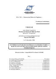
Fig. 1.1. illustrates a diminishing marginal rate of substitution between the 

x ‟s and q with quasi-concave utility functions. As q rises from 

increases from 

0 

u to 

39 

0 

q to 

1 

q , utility 

1 

u . Displacements of the indifference curves reflect unitary 

income elasticity. As can be seen, WTA � WTP . The trade-off between 

environmental quality and the private good turns out to be less and less attractive: the 

marginal utility from environmental quality upgrading is diminishing. Vice versa, it 

means that the marginal loss of environmental quality is increasing. In any case, the 

lower the elasticity of substitution between q and the x ‟s – or to be more accurate, 

between q and the x ‟s that y buys – the broader the disparity. 

WTA 

y 

WTP 

y 

0 

q 0 

Fig. 1.1. A change in q and imperfect substitution with the x ’s 

q 1 

� , , � 

1 1 

u � v p q y 

� , , � 

0 0 

u � v p q y 

q

Regarding the distance function, in presence of a normal good, the inverse 

0 

compensated demand curve � , , � 

1 

curve � , , � 

a x q u lies below the inverse compensated demand 

a x q u for the reason that scale effects depend on the elasticity of 

substitution between q and the x ‟s. In the presence of two goods, Park (1997) finds 

that the Hicks elasticity of substitution equals the Allen-Uzawa elasticity of 

substitution. The difference between WTP and WTA thus arises whenever 

substitutability is imperfect. 

What happens to the agent‟s behavior if we now distinguish foregone gains 

from real losses? 

1.4. Imperfect substitutability and the endowment effect 

Hanemann (1991) points out in his footnote 25 that Kahneman and Tversky‟s 

(1979) loss aversion, observed from some reference point, differs from the standard 

disparity. Indeed, in the Hicksian framework, preferences over consumption bundles 

are independent of initial endowments. In reference to the gain and loss perspective, 

Thaler (1980) proposed the term endowment effect. When an agent is endowed with a 

good, her reference point changes, she shifts her position on the map, and the shape of 

her indifference curve is altered. 

If we adapt the standard framework to the loss aversion idea, a gain or a loss 

in q can be written q � q � � and q � q � � , with 0 � � . Assume agent‟s utility is 

1 0 

� 

1 0 

� 

affected by variations of the environmental quality level q . In this case, her utility 

� , , � 

0 0 

u v p q y 

� , which now involves a single indifference curve, changes either to 

u � in a case of a gain or to u � in case of a loss: 

0 � , , � 

� 

u � v p q � � y 

[14a] 

0 � , , � 

� 

u � v p q � � y 

[14b] 

40

Bateman et al. (1997) define two additional measures, identified with some 

reference point. Regarding the first measure, the question is what additional amount 

of private consumption is as preferable as an increase in the environmental quality. 

This is the equivalent gain, equal to WTA. Regarding the second measure, the 

question is what loss of private consumption would be just as preferable as a decrease 

in the environmental quality. This is the equivalent loss, equal to WTP. 

When the agent is endowed, fixing a gain and a loss in [3a] and [3b] or [4a] 

and [4b] gives the following relationships: C � or compensating gain is the maximum 

amount she would pay to secure the gain; E � or equivalent gain is the minimum 

amount she would accept to sacrifice the gain; E � 

� or equivalent loss is the 

maximum amount she would give up to avoid the loss; C � 

� or compensating loss is 

the minimum amount she would accept to tolerate the loss. The summary is 

recapitulated in Table 1.2. 

Table 1.2. Welfare indices and context-dependence 

1 0 

1 0 

loss ( q � q � � ) gain ( q � q � � ) 

� 

� � 

�C�WTA�� 0� 

C WTP 

41 

� 

� �� 0� 

� � 

� � 

�E�WTP�� 0� 

E WTA 

� �� 0� 

� � 

� � 

� � 

Unlike the standard disparity alias �WTA � WTP � or �WTA WTP � 

� , where 

changes go in the same direction, a gain and loss disparity is computed differently, 

simply because we observe changes that depart in opposite directions from some 

reference point. Here, we subtract WTA to tolerate the loss and WTP to guarantee the 

� � 

gain or �WTA WTP � 

� . From [3a] and [3b], it follows: 

1 0 0 0 0 0 1 0 

� , �, � � , , � � , , � � , �, 

� 

� � 

�C �C � �e p q u � e p q u � � �e p q u �e 

p q u � 

� � � � [15a]

Since the utility function u �x, q� 

is quasi-concave in � q� 

0 

the expenditure function � , , � 

42 

x, , when q increases 

e p q u decreases, i.e. is convex in q , as less income is 

necessary to attain the fixed utility level. The second reaction is that the indirect 

utility function v �p, q, 

y� 

is quasi-concave in � y� 

q, , which means that the cross- 

2 2 

partial derivative only implies the substitution effect eqq � e q � 

� � � . As a matter of 

fact, the income effect – the spacing of the indifference curves – does not count, for 

gain and loss perspective involves a single indifference curve 

positive and negative change, thus: 

0 

u observed from some 

� � 

WTA � WTP � 0 

[15b] 

Proposition 1.2.: Imperfect substitutability between q and the x ‟s in the indirect 

utility function causes disparity either between WTP and WTA or between gain and 

loss, independently from the reference. 


Fig. 1.2. illustrates the four measures, observed from some reference 

0 

coordinates �q , y �. 

Grey curves depict the same pre-endowed utility 

0 

u observed 

from two reference points. Through the incursion of context-dependence, the utility 

changes from 

0 

u to either u � (a gain in utility) or u � (a loss in utility). The reference 

point for WTA � and WTP � is G. Viewed from G, the distance from 

0 

q to 

q � q � � 

1 0 

� 

is a gain in level of the environmental quality. For WTA � and WTP � the reference 

point is L. Viewed from L, the distance from 

0 

q to 

q � q � � is perceived as a loss 

1 0 

� 

in level of the environmental quality. The endowment effect induces the pivoting of 

the indifference curve from the reference point, which illustrates the discontinuity in 

the slope from 

0 

u to u � or u � . The steeper the indifference curve, the less the 

substitutability between q and the x ‟s that y buys.

The difference between WTA � and WTA � , which is essential to distinguish 

the standard disparity from the gain and loss disparity, lies in the way the loss is 

perceived. In the first case, the agent is asked to state her value to give up a gain from 

an increase in the environmental quality. This is an opportunity loss. This cannot be a 

right. In the second case, the agent is asked to state her value to suffer a loss from a 

decrease in environmental quality. This is a net loss and it differs from the former. 

. 

Fig. 1.2. Reference-dependent preferences 

The difference is due to imperfect substitutability, for agents take more account of the 

goods they can not regain. When agents are asked to value their losses in monetary 

terms, the behavioral effect of loss aversion arises and they shift their indifference 

curves. They know they have the right to be compensated for the loss and claim this 

right in form of high WTA � statements. 

� � � � 

Transitivity implies that whenever WTA > WTA and WTA > WTP , 

� � 

WTA > WTP . 

WTA – 

WTA + 

y 

WTP + 

WTP – 

y 

0 

G 

1 

q� 43 

1 

q� L 

q

1.5. Imperfect substitutability and loss aversion 

In their 1991 article, Tversky and Kahneman propose the behavioral 

reference-dependent theory as an alternative to the Hicksian theory of preferences. 

Outcomes are now valued using a value (utility) function where agents have 

preferences over goods relative to some reference level � x, q� 

44 

r r seen as the status quo. 

According to them, (i) all is perceived as a gain or a loss; (ii) losses are weighted 

more heavily than gains or agents are loss averse; and (iii) the marginal value of gains 

or losses exhibits diminishing sensitivity. They assume that preferences are transitive, 

continuous and nondecreasing (but not convex). 

r r stands for the reference points for consuming � q� 

If � x, q� 

function changes to u u� x, q, rx, rq� 

x, , the utility 

� ; the demand functions take the form of 

i 

i 

� � , , , , � and xi h � p, q, u, rx , rq 

� 

x h p q y r r 

i x q 

� ; the indirect utility is now 

v� p, q, y, rx, r q� 

just as is the expenditure function � , , , x, q� 

e p q y r r . These new 

functions are discontinuous at the reference point (Putler 1992). Fig. 1.3. shows a 

typical loss aversion curve observed within the context of welfare measurement. 

WTA – 

y�rx WTP + 

y 

0 

rq � 

q�rq rq � 

Fig. 1.3. Loss aversion in welfare measures 

q

The additive formulation of the constant loss aversion model used by Tversky 

and Kahneman gives the following indirect utility function: 

q y 

� , � R �i�q��i�y� u � v q y � � q � r � y � r � 

� � [16] 

with R' � 0. 

Parameters 

q 

� i and 

y 

� i , for 1,2 

i � and � � 1, 

are defined as coefficients 

of loss aversion for dimensions r q and r y . They magnify the disutility of losing some 

environmental quality. When the agent perceives a change as a gain, this coefficient 

amounts to 1 1 � � , which means that the agent has neoclassical utility. When she 

perceives a loss, this coefficient amounts to 2 >1 

y y 

2 1 

� � 

� > � � 1 . 

45 

i 

q q 

� . We can see that � > � �� 1�and 

2 1 

Definition 1.2.: The change from the reference level r q to either a gain rq � or a loss 

rq � , while ry� y, 

gives the following: 

q q y y 

�� i � �1 if q � rq � 0 and �i � �1 

if y � ry 

� 0 

� q q y y 

�� i � �2 if q � rq < 0 and �i � �2 

if y � ry 

� 0 

In terms of coefficients of loss aversion, the welfare measures matrix becomes 

what is shown in Table 1.3. 

Table 1.3. Welfare indices in a gain and loss perspective 

� � 

loss ( rq � rq 

� � ) gain ( rq � rq 

� � ) 

� � � � 1 2 WTP 

q y 

� � � � 

2 1 WTA 

q y 

� 

� � � � 1 1 WTA 

q y 

� � � � 

2 2 WTP 

q y 

� 

� 

�

q y 

Since �1 �1 

1 

� � , < 2 

q 

y � 

� 

� or 

� 

R �� , i.e. y � e�q, u� 

is the inverse of u v�q, y� 

2 

+ 

WTP < WTA � . If we invert the function 

46 

� with �R � y 

� 

differentiate it with respect to u , the following disparity arises: 

q 

�u� �u� i �q rq� 

�� ' if � �� 

eu �q, u� � �� 

'�u 

� 

� if � < � 

y 

� �2 

�1 

where � � � R � � 

q �u� i �q � rq� 

� � � and � '� 0. 

y� � r , and 

i y 

[17] 

The indirect utility function is quasi-concave because of the monotone 

transformation � � 

q 

R � in [16]. Moreover, i �q rq� 

� � is a concave function of q , which 

illustrates the gain and loss disparity with decreasing sensitivity to losses. Since 

2 >1 

y 

� , when q increases u 

e decreases, which implies the negativity of the derivative 

e qu from changes in q . As a result, we get back to the standard disparity between 

WTP and WTA. 

Recall that the curvature of the indifference curves shows diminishing 

marginal utility between the consumption bundles, and thus the standard WTA-WTP 

disparity. Furthermore, it generates disparity between gain and loss because of the 

imperfect substitution in the indirect utility function between y and some function of 

the environmental quality q . Through the discontinuity in the slope at the reference 

point, loss aversion theory implies convex indifference curves. On that subject, 

Hanemann (1999) argues that the assumption of quasi-concave utility function 

suffices to observe convexity. Quasi-concavity with inversely proportional disparity 

to the substitution effect can explain the disparity between gain and loss. The 

endowment effect within loss aversion can be explained through less than perfect 

substitutability.

The behavioral theory of loss aversion also works with distance effects. In 

terms of the distance function, it is a matter of distance between coordinates of some 

level of y or q and the agent‟s reference point. In this case, the function becomes 

� , , , x, q� 

d x q u r r . Adding coefficients of loss aversion into the distance function yields 

now a weighted distance function of the form: 

p p 

� � 

q y 

� , , � R �i�q��i�y� d � d x q u � q � r � y � r 

�� 

[18] 

where p � 1 denotes the metric. When p � 1, 

the distance is measured as the sum of 

weighted absolute differences. We then fall on [16]. The distance function recovers 

from the expenditure function. Therefore, imperfect substitutability can once again 

explain the gain and loss disparity. 

1.6. Imperfect substitutability and boundedness 

Randall and Stoll (1980) demonstrate that the disparity between WTP and 

WTA is bounded by the ratio between the price flexibility of income and endowment. 

Cook and Graham (1977) assert that the compensation demanded for irreplaceable 

commodities, which we can assume to be imperfectly substitutable, depends on the 

initial level of wealth or endowment. As the probability of loss p � 1, 

WTA, 

dependent on the income that buys the x‟s, tends to infinity as the indifference curve 

is asymptotic to the vertical line at p � 1. 

This is what Amiran and Hagen (2003) also 

suggest in a slightly different manner: in presence of asymptomatically bounded 

utility functions, there exists an initial level of wealth sufficiently high to produce an 

infinite WTA – . Nevertheless, the substitution effect still plays a capital role, for it 

induces frictional trade-off between public and private goods. In terms of elasticity, 

the authors show that the income elasticity of the inverse compensated demand is 

bounded above and below by positive values independent of the amounts of public 

goods. 

47

In case of reference-dependent preferences, we believe that imperfect 

substitutability accentuates the pivoting of the indifference curve, which in turn can 

produce infinite compensation demanded. We replace the nonsatiation assumption 

from Amiran and Hagen (2003) by the assumption that for each level of income y, the 

status quo q r is strictly preferred to some net loss of the public good rq �� with 

� >0 

or that u� rq , y� < u� rq, y� 

�� with r �� < r . A double outcome arises. The 

48 

q q 

first outcome lies in the convex curvature of the indifference curve. In point of fact, 

imperfect substitutability induces a steeper slope for higher opportunity losses (see 

Fig. 1.4.: grey segment and arrow 1). The second outcome results from the 

enlargement of the substitution effect due to aversion of net losses, yielding 

clockwise rotation and, accordingly, a steeper slope of the initial indifference curve 

(see Fig. 1.4.: black segment and arrow 2). 

Fig. 1.4. Unboundedness of the compensation demanded 

Beyond some level of loss of the public good �� 0 in view of their reference point, 

i.e. 

0 

q rq 

WTA – 

WTA + 

� � � , standard agents ask for an infinite monetary compensation. Formally, 

this yields a level of monetary compensation s – analogue to WTA – strictly inferior 

to the disutility of the loss: 

y 

y 

0 

2 

q 0 

1 

rq 

q

0 

� q, �> � q � > � , � 

u r y z r � � � s u q y 

[19] 

Proposition 1.3.: In case of reference-dependent preferences and imperfect 

substitutability between q and the x‟s that y buys, large net losses of the public good 

can be infinitely uncompensated. 


Hanemann (1999) points out that the wealth effect in Cook and Graham is not 

the income effect typically considered in consumer demand theory. While being true, 

let us recall that the income effect does not count within context-dependence. We 

therefore explain the infinite limit of WTA – by the pivoting of the indifference curve 

from the reference (endowed) level of the public good. Again, this is a net loss 

perception magnifying the substitution effect. Contrary to Cook and Graham who find 

infinite WTA – as the probability of losses moves towards one, our indifference curve 

is asymptotic to the vertical line at 

severe and approach 

0 

q , which shows infinite WTA – when losses are 

0 

q . Unlike the previous models – which unquestionably 

consider substitutability as the mainspring for infinite monetary compensation – our 

design neither depends on the initial level of wealth or the initial endowment in 

market goods nor on the boundedness of the utility function. It rather depends on the 

severity of loss of the public goods combined with their unfeasibility to be perfectly 

substitutable. 

In the behavioral loss aversion model, when an agent stands at � q, x� 

49 

r r , that is, 

at the kink point, q and y are perfect substitutes, for she is equidistant to both 

references points and indifferent between the level of environmental quality and her 

income. Except these coordinates, any other point along the curve exhibits imperfect 

substitutability. As can be noticed in terms of distance minimization, above the kink 

point she substitutes the loss of the environmental quality with monetary 

compensation. Below is the opposite. Because of loss aversion, as r � � � r

have �r r � v r 0 

� � � � � � . When rq �� goes farther from r q , additional decreases 

q q q 

in q lead to smaller changes in utility, which implies 

50 

2 2 

� v �q � 0 . In other terms, 

diminishing sensitivity implies a lower substitution effect in both gains and losses. 

Conversely to the standard model, the marginal disutility from environmental quality 

downgrading is decreasing as the agent moves from the reference point, implying a 

bounded value for compensation 8 . 

Proposition 1.4.: Inside the behavioral theory of loss aversion, given constant 

diminishing sensitivity towards losses, the substitution effect is bounded. 


Hence, there is a difference between the Hicksian standard paradigm and loss 

aversion in the representation of context-dependence. If we superpose the 

indifference curves illustrating the willingness-to-accept to tolerate a loss, their 

respective curvatures reveal two types of behavior on the subject of losses. The grey 

segment represents the standard theory context-dependence. The black segment 

stands for the behavioral model of loss aversion (see Fig. 1.5.). 

Inside the standard model, agents show increasing marginal disutility as 

rq �� tends towards 

0 

q . Inside the behavioral model, agents exhibit high loss 

aversion with small changes as regards their reference point, but they turn out to be 

less and less sensitive as 

r q 

0 

q � � � . Diminishing sensitivity of the marginal value of 

losses clarifies this phenomenon. The farther something moves from a reference 

point, the less additional changes should matter, which in our case surprisingly means 

increasing substitutability. This counter effect appears because agents are myopic, 

which makes them feel unconcerned by changes out of their visual field. As a 

consequence, they end up asking for a bounded amount of compensation, no matter 

the additional degradation of the environment. 

8 The shape of the losses is represented in a positive space because we deal with positive values of 

welfare indices.

WTA – 

y�rx Fig. 1.5. Comparison between reference-dependent indifference curves 

The significance of it is non-negligible. In case of irreversible damages to the 

environment or high losses of public goods with regards to their initial level – 

commodities that we know to be imperfectly substitutable –, standard agents which 

turn out to be far-sighted will ask for an infinite monetary compensation, whereas loss 

aversion agents will ask for a bounded amount of compensation, and neither can 

adapt their reference points. While economists have long considered loss aversion to 

degenerate agents‟ rational preferences, we see that past some level of changes in q, it 

limits their proclivity towards abnormal valuation. 

1.7. Concluding remarks 

Applied to market valuation of the public goods, this chapter dealt with 

imperfect substitutability in both standard welfare and reference-dependence theories. 

Imperfect substitutability in the indirect utility function can provoke disparity either 

between WTA and WTP or between gain and loss. Further, the same quasi-concave 

utility functions can explain the endowment effect. 

y 

0 

0 

q 

51 

rq 

q

What is the point of finding that imperfect substitutability plays a role in both 

the WTA and WTP disparity and the gain and loss disparity? According to the above, 

it basically means that agents‟ unwillingness to substitute an environmental good or 

service increases with its defective substitutability. When agents substitute a public 

good for a private good, an opportunity loss appears and induces the standard 

disparity. In case the scenario to price is a loss instead of a foregone gain, loss 

aversion transforms the opportunity loss in a net loss, which enlarges the initial 

disparity, for people heavily value things they cannot regain. Experimental findings 

from Boyce et al. (1992) and Chapman (1998) support this conclusion. At last, the 

substitution effect observed from some reference point has a bound inside the 

behavioral model of loss aversion. This could be tested in a laboratory. Whether 

agents should have infinite values for severe or irreversible losses might be the topic 

that decides which model better values environmental preferences. 

Yet, these common findings must be toned down. Valuing environmental 

goods or services calls for an understanding of the public and private benefits derived 

from the public good. This is partially ensured, as environmental commodities are 

unfamiliar to agents and their benefits for utility obscure in most cases. The risk of 

having naïve valuations is existent. Only an interactive market-like setting permits to 

surmount these limits, and hypothetical markets remain devoid of market interactions. 

Experimental markets are thus essential in the contingent valuation. In 

experimentation, the early disparity between welfare measures is redundant, 

supporting either of the two effects. But their confrontation occults the market 

efficiency which rules the economic valuation. Indeed, markets bound anomalies by 

means of ad hoc incentives, for they aid agents to correct their untruthful or naïve 

valuations. The next step consists in identifying, by probing into auction mechanisms, 

why some of them reduce the disparity better than others. As well, studying agents‟ 

context-dependent behavior faced with irreversible environmental damages and 

ambiguity – when they can adapt their reference points – is a matter of future 

research. 

1.8. References 

52

Amiran, E. and Hagen, D. (2003), “Willingness To Pay and Willingness To Accept: 

How Much Can They Differ? Comment”, American Economic Review, 93: 458– 

463. 

Bateman, I., Munro, A., Rhodes, B., Starmer, C. and Sugden, R. (1997), “A Test of 

the Theory of Reference-Dependent Preferences”, Quarterly Journal of 

Economics, 112: 479–505. 

Boyce, R., Brown, T., McClelland, G., Peterson, G. and Schulze, W. (1992), “An 

Experimental Examination of Intrinsic Values as a Source of the WTA-WTP 

Disparity”, American Economic Review, 82: 1366–1373. 

Blackorby, C., Primont, D. and Russell, R. (1978), “Duality, Separability and 

Functional Structure”, Theory and Economic Applications, North-Holland, New 

York. 

Brookshire, D. and Coursey, D. (1987), “Measuring the Value of a Public Good: An 

Empirical Comparison of Elicitation Procedures”, American Economic Review, 

77: 554–556. 

Cook, P. and Graham, D. (1977), “The Demand for Insurance and Protection: The 

Case of Irreplaceable Commodities”, Quarterly Journal of Economics, 91: 143– 

156. 

Chapman, G. (1998), “Similarity and Reluctance to Trade”, Journal of Behavioral 

Decision Making, 11: 47–58. 

Deaton, A. (1979), “The Distance Function in Consumer Behavior with Applications 

to Index Numbers and Optimal Taxation”, Review of Economic Studies, 46: 391– 

405. 

Ebert, U. (1984), “Exact Welfare Measures and Economic Index Numbers”, Journal 

of Economics, 44: 27–38. 

Ebert, U. (1993), “A Note on Willingness to Pay and Willingness to Accept”, Social 

Choice and Welfare, 10: 363–370. 

Hanemann, W. (1991), “Willingness to Pay and Willingness to Accept: How Much 

Can they Differ?”, American Economic Review, 81: 635–647. 

Hanemann, W. (1999), “The Economic Theory of WTP and WTA”, In Valuing the 

Environment Preferences: Theory and Practice of the Contingent Valuation 

Method in the US, EC and Developing Countries, edited by Ian Bateman and Ken 

Willis, Oxford: Oxford University Press. 

53

Hicks, J. (1943), “The Four Consumer‟s Surpluses”, Review of Economic Studies, 11: 

31–41. 

Kahneman, D. and Tversky, A. (1979), “Loss aversion in Riskless Choice: A 

Reference-Dependent Model”, Quarterly Journal of Economics, 106: 1039–1061. 

Kahneman, D., Knetsch, J. and Thaler, R. (1991) “Anomalies: The endowment effect, 

Loss Aversion, and Status Quo Bias”, Journal of Economic Perspectives, 5: 193– 

206. 

Knetsch, J. and Sinden, J. (1984), “Willingness to Pay and Compensation Demanded: 

Experimental Evidence of an Unexpected Disparity in Measures of Value”, 

Quarterly Journal of Economics, 99: 507–521. 

Mäler, K. (1974), Environmental Economics: A Theoretical Inquiry, John Hopkins 

University Press, Baltimore. 

Morrisson, G. (1997) “Resoving Differences in Willingness to Pay and Willingness to 

Accept: Comment”, American Economic Review, 87: 236–240. 

Park, H. (1997), “Randall and Stoll‟s Bound in an Inverse Demand System”, 

Economics Letters, 56: 281–286. 

Putler, D. (1992), “Incorporating Reference Point Effects into a Theory of Consumer 

Choice”, Marketing Science, 11: 287–309. 

Randall, A. and Stoll, J. (1980), “Consumer‟s Surplus in Commodity Space”, 

American Economic Review, 70: 449–455. 

Sinclair-Desgagné, B. (2005), “Calcul économique et développement durable”, Esprit 

critique, Vol. 07–N.01, available at http://www.espritcritique.fr. 

Thaler, R. (1980), “Toward a positive theory of consumer choice”, Journal of 

Economic Behavior and Organization, 1: 39–60. 

Tversky, A. and Kahneman, D. (1991), “Loss Aversion in Riskless Choice: A 

Reference-Dependent Model”, Quarterly Journal of Economics, 106: 1039–1061. 

54

1.9. Appendix 

Proof of Proposition 1.1. 

The demonstration is as follows. After Randall and Stoll (1980), WTP and WTA for 

changes in public goods should not differ with small income effects. They bound 

�E� C�via 

the income elasticity of demand (or income elasticity of willingness-to- 

pay) of the public good. For example, when the price of a certain good one changes, 

the disparity amounts: 

� 

1 

1 

1 0 

� , , � � , , � 

p 

� � 

p � p p � 

E �C � e p q u � e p q u dp 

or 

0 1 1 

1 

1 

1 1 

� � � � � � 

1 

� � � � 

E �C � e p, q, u � g p, q, u � g p, q, e p, q, u � e p, q, u 

p u u y u 

The income effect associated with good one – the second cross-partial derivative 

2 

epu e p1 u 

1 

� � � � – establishes the size of the disparity, the limit being the 

individual‟s income. The bounding method carries over to welfare measures of the 

quantity changes. The analogous result for a change in q gives the cross-partial 

derivative 

market goods: 

� 

q 

2 

equ e q u 

1 

� � � � , i.e. the substitutability of the nonmarket good by means of 

0 1 

� , , � � , , � � , , � 

E �C � �e 0 

q 

q p q u eq p q u � 

� 

� 

� 

dq � �equ 

p q u 

For a change in the public good‟s level, Hanemann (1991) demonstrates that the 

second cross-partial derivative e qu reflects the substitution effect. Indeed, from [8] 

and the differentiation of the compensating demand function for q , we hold the 

derivative involved in changes in q that impact on u : 

55

� , , � 

e p q u 

g � p, �, e p, �, u �� e� p, �, 

u� 

� , �, , � , � y � , �, 

� 

� p, q, u� 

q 

y � � 

� � 

2 

� e �� 

ˆ ˆ 

� � � 

�q�u �u gˆ p eˆ p u �gˆpu�q qu q 

� 

q 

By the Hicks decomposition, the precedent becomes: 

� � � 

� � � 

q 

gˆ u p, , u 

equ � p, q, u� 

= q 

gˆ p, , u 

� 

This difference between WTP and WTA depends on the price flexibility of income 

and thus the ratio of the income elasticity of the ordinary demand function for q to 

the elasticity of substitution between q and the x ‟s 9 . The numerator represents the 

income effect of q in the hypothetical market, established from the derivative of the 

demand function with respect to income. The denominator is the own-price derivative 

of the compensated demand function for q and gives the aggregate Allen-Uzawa 

elasticity of substitution between q and the private goods weighted by the budget 

share of the same private goods. 

Changes in prices and changes in q both vary with income and depend on a cross- 

partial derivative of the expenditure function. And when e qu

A necessary and sufficient condition for the disparity between gain and loss to occur, 

i.e. WTA > WTP 

� � 

, is that v �p, q, 

y� 

is quasi-concave in � y� 

57 

0 

p, or that � , , � 

e p q u is a 

convex function of q . In this case, the second partial derivative e qq must be strictly 

positive. Let us look at the expenditure function. 

The disparity arises because of the convexity of the initial indifference curve 

follows from [3a] and [3b] that: 

1 0 0 0 0 0 1 0 

� , �, � � , , � � , , � � , �, 

� 

� � 

�C �C � �e p q u � e p q u � � �e p q u �e 

p q u � 

� � � � 

Which gives: 

1 0 1 0 0 0 

0 � e� p, q�, u � � e� p, q�, u � � 2 e� p, q , u � 

� 0 0 � � � 0 

� � 

0 � � � 0 

� � 

0 � 

2 e p, q , u e p, q , u e p, q , u 

� � 

1 

e p q u e p q u e p q u 

2 

0 0 0 0 0 0 

� , , � � � , � �, � � � , � �, 

� 

0 0 

In parallel, � , , � 

e p q u can be rewritten as: 

�� 

� 1 0 0 0 � 

e�p, q q , u � 

� 2 

� 

Substituting the precedent into the general inequality gives: 

0 0 0 0 0 0 0 

�� 

� � 

� 1 � 1 

e� p, q q , u � e p, q , u e p, q , u 

� 2 � 2 

� 1 1 � 1 1 

e� p, q �1 � q , u � e p, q , u �1 �e 

p, q , u 

� 2 � 2 � � 

2 � 2 � 

0 � � 0 0 0 0 � � 0 0 

� � �� 

0 

u . It

From which directly follows the convexity of the expenditure function of q . The 

expenditure function being convex, we have e qq >0. 

There is a disparity between gain and loss. � 


For 

0 

q rq rq 

� � � � with >0 

� 

us set z �q� �sup y u �q, y� �u�rq, 

y� 

� 

0 

� , we have u0 � u �rq , y� 

and u �q, y� u �q , y� 

58 

� . Let 

� � 

� � 

for a level of monetary compensation such 

that the utility remains constant. For each 0 

q � we have z �q� u� q, y� 

� . The 

supremum z�q � is increasing in q. This says that for each level of income y and for 

0 

q � we have u� rq, y� u� rq , y� 

r q 

the net loss of the public good � . 

Let us set � � � �= 

q q 

� � � because the status quo is always preferred to 

z r � z r � � s where s > � is the compensation analogue to WTA. 

With z�r q � being the supremum for u �rq , y � and � q � 

z r �� being the supremum for 

0 � q �� , � is there y that gives u� q , y� > z �rq �� or � q, �> � q � 

u r y 

We know that 

0 

q rq rq 

u r y z r � � � s ? 

0 

� � � � so for all y we have z �q � z �rq � 

0 � � � � q � � � . By definition we know that z �rq � s z �rq� z q z r 

0 

0 0 � � � � � q � holds. Moreover, z �q � u� q , y� 

z q s z r 

0 0 0 � � � � � , � or z �rq � s u �q , y� 

z q s u q y 

As 

� � � � . 

0 

0 

q � we have z �rq � z �q � 

r q 

0 

� q, 

� � � 

u r y � z q � s . 

� and 

� � � � such that 

� because z �q� u� q, y� 

0 

� � � or z �rq � s z �q � 

� thus 

� � hence

0 

From the above we see that u� q , y� < z �rq � s u �rq, y� 


59 

� � � � � 

Let us now prove that WTA is bounded within the behavioral model of loss aversion. 

One way comes directly from the construction of the model: according to diminishing 

sensitivity, smaller changes in � should be accompanied by smaller increases in y , 

the utility being constant, thus 

2 2 

� u �q � 0. 

��rq � �� 0, r � q� 

and some value function * 

v C�R�� on �0, r � q � which is concave 

and nonincreasing, one has: v�r q � v'� rq ��rq rq � v�r q � 

� � � � � � � . The right-hand 

expression of the weak inequality is the tangent of v at r q . It gives 

� q � '� 

q �� q � � q � 

v r � � � v r �r � v r when rq � � � 0 which is independent of rq ��. 

Hence, the losses‟ side of the value function is bounded. �

61 

Chapter 2 

Private Valuation of a Public Good 

in Three Auction Mechanisms 

Abstract 

We evaluate the impact of three auction mechanisms – the Becker–DeGroot– 

Marschak (BDM) mechanism, the second-price auction, and the random nth-price 

auction – in the measurement of private willingness-to-pay and willingness-to-accept 

for a pure public good. Our results show that the endowment effect can be eliminated 

with repetitions of the BDM mechanism. Yet, on a logarithmic scale, the random nthprice 

auction yields the highest speed of convergence to welfare indices‟ equality. 

Overall, we observe that subjects value public goods in reference to their private 

subjective benefit derived from the public good funding. 

Keywords: contingent valuation, WTP-WTA gap, auctions, public good private 

provision 

JEL classification: C91, D44, Q53


62 

"I have never known much good done 

by those who affected to trade for the 

public good." Adam Smith 

The experimental private provision of public goods based on the contingent 

valuation method is often used to value public goods such as health, safety or 

environment. Estimating preferences for public goods is however laborious, for 

individuals reveal behavioral biases during their valuation process. 

In accordance with the Coase theorem (Coase 1960), neoclassical theory 

postulates that with null income effect and close substitutes, the willingness-to-pay 

(WTP), which is the price at which an individual is ready to buy a commodity, and 

the willingness-to-accept (WTA), which is the price at which an individual is ready to 

sell the same commodity, should be equal (Randall and Stoll 1980, Hanemann 1991). 

If the good is available in an active market at the market price, an individual‟s WTP 

and WTA should be similar. And if people face similar transaction costs, WTP and 

WTA should be similar among people as well. Yet, experimental research that 

stemmed from contingent valuation studies has found large disparities between the 

WTP and WTA. The endowment effect, or loss aversion, as a behavioral feature is 

often invoked to explain the disparity. It occurs when people offer to sell a commonly 

available good in their possession at a substantially higher rate than they will pay for 

the identical good not in their possession. The other effect, promoted to explain the 

disparity, is imperfect substitutability. 

Two remedies help remove the initial disparity. The first corresponds to 

market settings. Market institutions serve as social tools that induce and reinforce 

individual rationality (Smith 1991). Gode and Sunder (1993) assert that an auction 

market exerts a powerful constraining force on individual behavior. Cherry et al. 

(2003) suggest that a dynamic market environment with repeated exposure to 

discipline is necessary to achieve rationality. When they act rationally, individuals 

refine their statements of value. List (2003a) provides evidence consistent with the 

notion that experience in bidding with an incentive-compatible auction can remove

the WTA/WTP gap. The second corresponds to market repetition. The motive for 

repeating auctions that are incentive-compatible is that individuals require experience 

to understand that sincere bidding is the dominant strategy (Coppinger et al. 1980) 

and to realize their true valuation of unfamiliar products (Shogren et al. 2000). Plott 

(1996) advances a discovered preference hypothesis argument, positing that 

responses reflect a type of internal search process in which subjects use practice 

rounds to discover their preferences. The experience they gain is reflected in their 

bidding behavior. Hence, the imperfect substitutability effect disappears when the 

value of the unfamiliar good is perfectly revealed. 

Market-based mechanisms such as auctions are widely studied as a means of 

buying and selling resources. Auctions took part in the environmental valuation to 

answer two questions: (1) which effect counts the most in the WTP and WTA 

disparity? and (2) which of the auction mechanisms best removes this disparity? 

At first, Kahneman et al. (1990) report experimental evidence of the 

endowment effect. They perform an experiment on WTP and WTA by way of 

hypothetical telephone inquiry, trading environmental improvements and 

preparedness for disasters. They find that randomly assigned owners of an item 

require more money to separate from their possession than random buyers are willing 

to pay to acquire it. To elicit individuals‟ estimates, they use a Becker-DeGroot- 

Marschak mechanism (BDM) – described later on – with random exogenous price 

feedback. According to their results, preferences are dependent on endowments, even 

in market settings. 

Shogren et al. (1994) assert that Kahneman et al.‟s experiment creates 

artificial scarcity. They find no evidence of the endowment effect on trading candy 

bars, for the values converge over time. But, in the experiment with contaminated 

food – a good with imperfect substitutes that can be considered as nonmarketed – 

they show that the discrepancy remains significant after iteration. 

Later on, Shogren et al. (2001) test three auction mechanisms to trade candy 

bars and mugs and suggest that the auction mechanism can itself account for the 

conflicting observations in experiments. In their experiments, they show that the 

common early disparity between WTP and WTA in auctions is not to be called into 

63

question. However, the gap ebbs away under the Vickrey‟s second price auction 

(SPA) and random nth-price auction (NPA) – see Section 2 for further details – while 

it lasts under the BDM mechanism, implying that the endowment effect can be 

eliminated with repetitions of some market mechanisms. 

Horowitz (2006a) states that the BDM framework could be used to assess 

public WTP for public projects, with the distribution of costs equal to the project 

costs; and other valuation mechanism should be used if the behavioral evidence 

shows that mechanisms are equivalent. Lusk and Rousu (2006) suggest that NPA is 

preferable to BDM if the researcher is looking for true valuation above all. Lusk et al. 

(2007) conclude in their study of payoff functions that BDM and NPA "provide 

relatively strong incentives for truthful bidding for all individuals regardless of the 

magnitude of their true WTP". 

Seeing that findings suggest that the auction mechanism per se accounts for 

the conflicting observations across market settings, Plott and Zeiler‟s (2005) 

conclusion that the results differ from unsound experimental procedures is 

incomplete. 

This chapter builds on Shogren et al.‟s (2001) results. Which auction 

mechanism is the best and fastest at reducing the gap? Which mechanism should be 

preferred over another? While Shogren et al. (1994) support Hanneman‟s results, 

assuming that the low substitution elasticity for the nonmarket good explains the 

WTA/WTP gap, they do not advocate the institution capable of properly valuing 

nonmarket goods. Likewise, Shogren et al. (2001) use only private goods to compare 

the influence of auction mechanisms. Only List (2003b) gives credit to the use of the 

random nth-price auction in valuing nonmarket private goods, but he does not state 

whether his results carry over to public goods. 

We aim at studying private valuation of public goods without direct 

substitutes, so we put realistic public goods such as the carbon offset, which can be 

attained via tree planting, into auctioning. Public goods have two defining 

characteristics: non-excludability and non-rivalry. Offsetting carbon emission helps 

prevent the effects of climate change; it is considered as a public good because, once 

provided, everyone can enjoy the benefits without adversely affecting anyone else‟s 

64

ability to do the same 10 . Rather then compulsory carbon trade, we institute voluntary 

trade to approach truthful valuation on both the bidder‟s (buyer‟s) and the offerer‟s 

(seller‟s) sides. On account of the common bias of nescience 11 in valuing unfamiliar 

or public goods, we remind the subjects that they are part of the milieu, which makes 

them indirectly and partly accountable for the current level of greenhouse gases, as 

they solicit industries to produce goods they are willing to consume at some 

environmental cost; in our case, it is the paper and energy used by students to achieve 

their education 12 . 

By means of repetitive auction mechanisms, the initial disparity between WTP 

and WTA can be removed. Nevertheless, we obtain different results from preceding 

studies, in a sense that only the BDM mechanism is able to remove the gap in later 

bidding rounds. SPA and NPA, which are also incentive-compatible, do not succeed 

in removing the disparity between bids and offers. Still, when we submit our 

experimental results to the exponential regression, we notice that in spite of a large 

early gap, NPA yields the highest speed of convergence to welfare indices‟ equality, 

suggesting that it contains strong incentives for rational behavior. In addition, we 

observe that subjects are strongly motivated by the subjective private benefit from 

funding the public good (either due to warm-glow 13 or to a concern for being 

formally identified as a contributor of the public good). 

The remainder of this chapter proceeds as follows. Section 2.2 describes the 

experimental design. Section 2.3 presents results and the analysis of data through 

standard and novel statistical tools. Section 2.4 provides discussion on how our 

results relate with existing work and present a new line of reasoning. We give some 

concluding remarks in Section 2.5. 

10 We insured the public good characteristic by providing to every subject, after couple of weeks, an 

email feedback on the aggregate offset achievement. 

11 It reflects the absence of knowledge or the consideration that things are unknowable. 

12 The money released from trading (buying and non-selling) was sent to a non-governmental 

organization that launched a plantation of 1,404 Mangrove trees in Sumatra, Indonesia. 

13 Utility derived from the warm-glow (see Andreoni 1990) arises when the act itself of giving 

generates utility. It contrasts with the usual case where the individual only cares about the total amount 

of the carbon offset. 

65

2.2. The experimental design 

We want to evaluate the impact of three incentive-compatible auction 

mechanisms in the measurement of WTP and WTA for a public good without 

substitutes. Our experiments were conducted during three sessions at the École 

Polytechnique. Different subjects took part in each of the three sessions (three types 

of auction mechanism) for a total of 102 participants, divided in three groups of 

subjects, which in turn were arbitrarily divided into two subgroups of buyers and 

sellers. Each subject received an identification number she filled in on each bid or 

offer, enabling her to be tracked whilst preserving her anonymity. The initial 

endowment distributed to the buyers was put forward to fund tree planting. On the 

WTP market-side, each buyer received EUR 15 and was asked to state her bid for a 

certificate of one ton of carbon offset (≤ EUR 15). If she won the bid, trees were 

planted in her name (this was acknowledged by a certificate). On the WTA market- 

side, each seller was given a certificate of one ton of carbon offset she could keep, in 

which case trees were planted in her name, or sell. If she decided to sell the certificate 

on the offer she stated (≤ EUR 15), no trees were planted. Subjects ignored that the 

cost of offsetting one ton of carbon in a five-year period was EUR 15, which enabled 

to plant 36 trees 14 . 

The parameters – recapitulated in the table below – of the experiments are the 

following: (i) 31 to 37 subjects participated per experiment; (ii) subjects were 

recruited among the voluntary students from the École Polytechnique 15 ; (iii) the good 

put in auctioning was a certificate of one ton of carbon offset; (iv) none information 

on price was provided; (v) subjects received an initial balance of EUR 15 or a 

certificate of one ton of carbon offset as an endowment; (vi) ten trials per experiment 

were unfolded, one of which was randomly selected as the binding trial; and (vii) 

BDM, SPA and NPA auction mechanisms were tested. 

14 In accordance with the system of reference applied by the non-governmental organization. 

15 Multi-cultural elite undergraduate students in science and engineering, salaried by the French 

Government. Their curriculum includes economics courses. 

66

Comments on the experimental protocol: our goal is to question auction 

mechanisms‟ influence on the gap between WTP and WTA, and not to divulge the 

gap itself, for we consider it as an established fact, so we decide to put an upper- 

bound on the sellers‟ choices in order to monitor which of the three market settings 

best replies to the early disparity. The bounds and endowments definitely create an 

anchoring effect, but there is no reason that it affects differently the three incentive- 

compatible mechanisms. Then, we publicly suggested to the subjects that revealing 

truthful preferences is a neutral strategy which will not penalize them. At last, we 

pooled all performed rounds in the measurement of the gap. 

Market environment BDM SPA NPA 

Auctioned goods CO 2 offset certificate CO 2 offset certificate CO 2 offset certificate 

Initially endowment EUR 15 EUR 15 EUR 15 

Sellers‟ bound EUR 15 EUR 15 EUR 15 

Number of trials 10 10 10 

Retail price information None provided None provided None provided 

Optimal responses explained Suggested Suggested Suggested 

Practice round performed Pooled Pooled Pooled 

Subject participation Voluntary Voluntary Voluntary 

Number of subjects 37 34 31 

The Becker–DeGroot–Marschak mechanism (BDM) 

Becker, DeGroot, and Marschak (1964) introduce a mechanism under which 

buyers (respectively sellers) simultaneously state the highest (respectively lowest) 

amount they are willing to pay (respectively accept) for the good. In our experiment, 

each buyer and seller was asked to give, for each of the ten trials, independently and 

privately, her WTP or WTA by marking an "x" on a recording sheet that listed price 

intervals, such as in the following illustration. The price intervals ranged from EUR 

1–15, in increments of EUR 0.5. After collecting recording sheets from buyers and 

sellers, the monitor randomly selected one price from the list. If a buyer was willing 

to pay at least the random price for the certificate of one ton of carbon offset, she 

bought the item at that price. Otherwise, she did not buy the item. If a seller was 

67

willing to accept a price lower than or equal to the random price for the certificate of 

one ton of carbon offset, she sold the item at that price. Otherwise, she did not sell the 

item. 

I will buy (sell) I will not buy (sell) 

If the price is EUR 0.0 -- -- 




… 




The random price, all bids and offers, and the number of buyers and sellers 

willing to buy and sell at the random price were made public after each trial. At the 

end of the experiment, one of the trials was randomly selected as the binding trial for 

the take-home pay. 

The second-price auction mechanism (SPA) 

Under the Vickrey (1961) second-price auction, bidders and offerers operated 

simultaneously. Buyers were asked to record, for each of the ten trials, privately and 

independently, the maximum they were willing to pay for the certificate of one ton of 

carbon offset. In this case, buyers wrote a numerical value on the recording sheet. The 

monitor collected values and, after each trial, made all bids public, as well as the 

identification number of the highest bidder and the market-clearing price (second 

highest bid). The monitor gave each seller a certificate of one ton of carbon offset. 

For each trial, sellers wrote their minimum WTA to sell the certificate. After each 

trial, the monitor publicly diffused all offers, the identification number of the lowest 

offerer and the market-clearing price (second lowest offer). Like with BDM, after the 

tenth trial, the monitor randomly selected one of the trials as the binding trial for the 

take-home pay for both buyers and sellers. 

68

The random nth-price auction mechanism (NPA) 

The random nth-price auction is conducted as follows (bidders and offerers 

operate simultaneously): (i) for each trial, each bidder submits a bid (resp. an offer) 

on a recording sheet; (ii) all bids are ranked from lowest to highest, all offers are 

ranked from highest to lowest; (iii) the monitor selects a random number n� �2, N� 

with N the number of bidders; (iv) the n � 1 buyers who made the highest bids buy the 

certificate of one ton of carbon offset at the nth-price and the n � 1 sellers who made 

the lowest offers sell the certificate of one ton of carbon offset at the nth-price. The 

value of n, all bids and offers, the buying and selling price, and the number of buyers 

and sellers willing to buy and sell at the random price, are made public after each 

trial. Once again, after the tenth trial, the monitor randomly selects one of the trials as 

the binding trial for the take-home pay for both buyers and sellers. 

The BDM, SPA and NPA mechanisms are incentive-compatible. It is not in a 

buyer‟s interest to understate her WTP; if the random buying price falls between the 

stated WTP and the true WTP, the buyer foregoes a beneficial trade. It is also not in a 

buyer‟s interest to overstate true WTP; if the random buying price is greater than the 

true value but less than the stated value, the buyer is required to buy the good at a 

price greater than her true WTP. The reasoning is identical for the seller. 

A complementary remark on NPA can be made. Contrary to SPA, subjects 

have a nonnegative probability of winning the auction, which engages off-margin 

bidders and offerers who usually consider that they will be excluded from the market. 

As well, the endogenously determined market-clearing price prevents bidders and 

offerers from using the random market-clearing price as an indicator. 

2.3. The results 

Table 2.1. presents the summary statistics of the experimental results under 

BDM, SPA and NPA. In all experiments, bidding behavior in the initial trial does 

69

Auction Value measure 

Table 2.1. Summary statistics of the BDM, SPA and NPA mechanisms 

H0: Mean WTP – Mean WTA = 0; H1: Mean WTP – Mean WTA < 0 

a t-test: reject H0 at the 5% level 

Trial 

1 2 3 4 5 6 7 8 9 10 

BDM WTP Mean 6.18 7.11 7.82 8.11 8.29 8.66 8.39 8.71 8.82 8.61 

N=19 Median 5.00 5.50 6.50 6.50 7.00 7.00 7.00 7.50 7.50 7.50 

Variance 12.51 15.52 15.39 15.43 15.09 15.86 15.27 14.62 14.37 17.74 

WTA Mean 10.53 9.47 9.56 8.42 8.92 8.69 9.53 9.19 8.67 8.06 

N=18 Median 10.00 10.00 10.00 8.75 9.50 9.75 10.00 10.00 9.75 8.25 

Variance 6.07 12.34 18.03 18.60 20.95 21.53 19.75 16.86 17.79 20.97 

Ratio of mean WTA/WTP 1.70 1.33 1.22 1.04 1.08 1.00 1.13 1.06 0.98 0.94 

t-test of means a –3.85 –1.46 –0.83 0.27 0.06 0.46 –0.39 0.09 0.58 0.91 

SPA WTP Mean 3.47 3.91 4.69 5.43 5.68 5.71 6.01 6.50 5.46 6.59 

N=17 Median 3.00 4.10 5.00 5.60 5.80 6.05 7.00 7.00 7.00 7.00 

Variance 9.64 6.68 5.52 5.42 6.15 7.71 8.86 14.50 12.56 10.04 

WTA Mean 10.66 8.74 8.47 9.07 8.59 9.82 9.40 8.32 9.52 9.23 

N=17 Median 10.00 9.00 8.00 9.00 7.00 10.00 8.00 8.00 8.00 8.00 

Variance 16.60 19.56 14.03 22.27 20.72 29.45 29.44 32.86 26.44 30.86 


t-test of means a –5.28 –3.41 –3.06 –2.35 –1.78 –2.30 –1.78 –0.59 –2.21 –1.20 

NPA WTP Mean 3.97 3.98 4.77 4.93 4.77 5.19 6.18 6.12 6.85 6.72 

N=15 Median 2.50 4.00 5.00 5.12 5.14 5.01 7.00 6.50 7.00 7.26 

Variance 12.67 6.92 4.83 4.30 5.40 6.33 5.81 6.54 7.77 10.03 

WTA Mean 10.75 10.52 10.29 10.22 9.86 9.05 9.17 9.14 9.23 9.37 

N=16 Median 10.50 10.00 9.74 9.65 8.77 8.50 8.49 8.35 8.09 8.50 

Variance 10.19 6.99 6.32 9.46 10.31 13.75 16.67 13.30 14.08 20.64 


t-test of means a –5.06 –6.45 –6.21 –5.17 –4.60 –2.87 –1.90 –2.10 –1.40 –1.33 

70

not contradict the endowment effect: the mean offer WTA 16 is significantly 

greater than the mean bid WTP 17 . Still, with experience gained through repetitive 

auctioning under the BDM mechanism, WTA offers decrease and WTP bids 

increase over time 18 . The WTA / WTP ratios thus decline throughout the ten 

trials, falling from 1.70 in trial 1 to 0.94 in trial 10 (see Fig 2.1.), which 

corresponds to WTP increase of 39% and WTA decrease of 23%. Concerning 

variances, we notice that the dispersion around the mean increases for both WTP 

(42%) and WTA (245%) from trial 1 to trial 10. In trials 4–10, a t-test shows that 

we cannot reject the null hypothesis that WTP and WTA come from the same 

distribution at the p

3,50 

3,00 

2,50 

2,00 

1,50 

1,00 

0,50 

1 2 3 4 5 6 7 8 9 10 

Fig. 2.1. WTA / WTP disparity from trial 1 to trial 10 

Let us now take a further insight in our results and those of the mug 

experiments from Shogren et al. (2001). At first sight, we obtain contradictory 

results. In our experiment, the gap disappears under BDM, whereas in theirs, 

BDM is the only mechanism unable to remove the early gap. 

Our findings show that repetitions under the BDM mechanism can remove 

the endowment effect, as long as it steers people‟s behavior. Likewise, they 

suggest that the auction mechanism per se can account for the conflicting 

observations, as we clearly observe different paths of equalization of WTP and 

WTA . We introduce an innovative tool to study the path of gap removal: the 

exponential regression on the WTA / WTP ratios. 

An exponential regression is of a form 

72 

BDM 

SPA 

NPA 

ax 

y � be with x the variable along 

the x-axis, y the regressed values of WTA / WTP , a the amplitude of the 

decrease (or speed of convergence to equality) and b the y-intercept of regression. 

The function is based on the function linear regression, with the y-axis 

logarithmically scaled. R-square gives information on the exponential relationship 

between ratios. 

We apply this method to Shogren et al.‟s (2001) mug experiments (see 

Fig. 2.2.) and to our experiments (see Fig. 2.3.). The exponential regression is

used for two reasons: first, it allows observing phenomena with rapid variations, 

such as in our experiments; second, it allows observing the decrease path to 

equality, that is, the way ratios tend to one. We try to unearth the mechanism able 

to remove the gap as quickly as possible, whatever the initial ratio. We can thus 

consider the highest coefficient of decrease as the highest speed of convergence to 

welfare indices‟ equality (see Table 2.2.). 

3,50 

3,00 

2,50 

2,00 

1,50 

1,00 

0,50 

3,5 

3 

2,5 

2 

1,5 

1 

0,5 

0 1 2 3 4 5 6 7 8 9 10 

Fig. 2.2. Exponential regression of WTA / WTP disparity 

from Shogren et al.’s (2001) mug experiments 

0 1 2 3 4 5 6 7 8 9 10 

Fig. 2.3. Exponential regression of WTA / WTP disparity 

73 

BDM 

SPA 

NP A 

Expon. (NP A) 

Expon. (S P A) 

Expon. (BDM) 

BDM 

SPA 

NP A 

Expon. (S P A) 

Expon. (BDM) 

Expon. (NP A)

Shogren et al.‟s (2001) data from BDM provides no exponential 

relationship between sequential ratios, but ours does. Although the y-intercept of 

regression starts with the same value (both 1.5), the gap disappears in our 

experiment (illustrated by the speed of convergence –0.04) but stays stationary in 

the mug experiment (null speed of convergence). 

We find in both data that NPA provides the best exponential relationship 

between ratios (respectively 

2 

R � 0.95 and 

74 

2 

R � 0.96 ) and the highest speed of 

convergence to equality (respectively –0.08 and –0.12) in time. Under SPA, the 

exponential relationship between ratios (respectively 

2 

R � 0.61 and 

2 

R � 0.63) 

and the speed of convergence to equality (respectively –0.06 and –0.09) are 

significant but lower. Sudden leaps of increase of the WTA / WTP ratio under 

SPA – due to off-margin bidders – explain the differences in 

2 

R with regard to 

NPA. It is worthwhile noticing that SPA comes out as the "worst" active market 

mechanism even though it is frequently used in experimental environments to 

reveal agents‟ preferences. Under BDM, our experiment and Shogren et al.‟s 

(2001) experiment both obtain the lowest results in terms of exponential 

relationship 19 and speed of convergence to equality. Therefore, the orderings of 

convergence in our experiments and those of Shogren et al.‟s (2001) are alike. 

Table 2.2. Exponential regression statistics 

Auction Regression statistics Our experiments 

Shogren et al.’s 

mug experiments 

BDM Speed of convergence (a) –0.04 –0.00 

y-intercept of regression (b) 1.5 1.5 

R-square 0.69 0.00 

SPA Speed of convergence (a) –0.06 –0.09 


R-square 0.61 0.63 

NPA Speed of convergence (a) –0.08 –0.12 


R-square 0.95 0.96 

19 The low exponential factor with the BDM is partially explained by the initial smaller difference 

between WTP and WTA.

If the initial gap is due to the choice of the market mechanism, then the 

choice of BDM is appropriate, for it produces the smallest initial gap. But, if we 

are to urge the auction mechanism able to rapidly deflate an excessive initial 

WTA / WTP gap in a market-clearing price setting, we suggest the use of NPA 

which involves most of the bidders in the auctioning. Indeed, as for the model of 

exponential regression, the BDM mechanism would not have equalized the 

welfare indices if the starting ratio were more of SPA or NPA‟s magnitude. This 

appears all the more sound, provided the BDM mechanism is a passive market- 

like setting with only minor adjustments in bidding behavior 20 . Indeed, NPA 

applies competitive pressure to the participating bidders. A bidder cannot avoid 

acting strategically since her best bid depends on the competing bids. By bidding 

more aggressively, the bidder improves her chances of winning the auction. As far 

as SPA is concerned, the unevenness in the decrease of the gap jeopardizes its 

robustness. 

2.4. Discussion 

Our results support the standard thesis that market mechanisms can 

remove or at least sturdily reduce the initial disparity between WTP and WTA. 

However, some points need to be clarified. 

Let us first focus on the specificity of the good in sale. Under NPA and 

SPA, the number of traded tons of carbon offset in a period is independent of the 

bids and offers submitted by the subjects. In any case, in SPA, one ton of carbon 

offset is bought and sold; in NPA, n � 1 tons of carbon offset are bought and sold. 

As a result, free-riding is likely to occur, since a subject‟s bid cannot affect the 

total public good provision while it affects her payment (buying a certificate is 

costly). On the contrary, under BDM, subjects‟ choices affect the total provision 

of public good. Indeed, if a seller chooses a minimum selling price higher than the 

randomly selected price, she will keep her certificate and one more ton of carbon 

20 See footnote 7 in Shogren et al. (2001). 

75

will be offset. The same reasoning applies for buyers. Put differently, subjects 

know they can influence the amount of carbon offset under BDM as their 

probability of winning the right to buy one certificate is independent of other 

bidders: the higher the private bid, the higher the chances that a ton of carbon is 

offset. 

This difference between BDM on the one side and NPA and SPA on the 

other side allows identifying two distinct motivations for funding the public good. 

First, there is "the public good motivation": a subject wants to buy or keep a 

certificate because it allows offsetting one ton of carbon for the community. 

Second, there is "the private good motivation": a subject wants to buy or keep a 

certificate because she wants to own a certificate and be associated to the 

offsetting even though this does not change the number of tons of carbon offset 

(she either wants to derive a warm-glow from altruism or wants to gain social 

status through the public good funding). Individuals often provide more public 

goods than traditional economic theory predicts. Public goods are then considered 

as impure public goods, which are products or services that combine both public 

and private benefits. 

In BDM, both motivations for funding the public good are present, 

whereas in NPA and SPA, only the private good motivation is present. Let us 

consider s – the mean value of all bids (WTP) and offers (WTA) – as the mean 

value of the public good. After computation, we observe that s over the ten 

rounds is strictly higher with BDM (8.57) than with SPA (7.26) or NPA (7.63). 

Locally, at the last period, the values are respectively 8.34, 7.91 and 8.09. These 

results indicate that the private good motivation is extreme compared to the public 

good motivation, i.e. subjects are mainly paying for enjoying warm-glow or being 

identified as contributors of the carbon offsetting. If we take s of BDM as a 

benchmark value of the public good, the surplus of the BDM value compared to 

SPA and NPA values corresponds to the value of the public good motivation 

which lies in the interval �0.94, 1.31 �. 

Since the public benefit for an individual is 

negligible, individuals mostly derive some private benefit from the public good. 

76

These results are thus consistent with microeconomic analysis, where the private 

benefit governs the decisions of economic agents. 

Contrary to the observations where repeat-play public good games produce 

declining contribution over time (see Andreoni (1988) and Caldas et al. (2003)), 

s is increasing in our experiments. As a matter of fact, if we regress s with the 

number of periods, we obtain a small but strictly positive correlation coefficient 

(BDM: 0.18; SPA: 0.13; NPA: 0.15). In standard public good games, the fall is 

motivated by free-riding and discouragement of high type players to pursue alone 

the provision of public good. We propose two explanations for the rise we 

observed. First, the funded public good does not only concern the subjects but the 

population outside the experiment. Therefore, the free-riding attitude of some 

participants does not alter subjects‟ motivations since they do not specifically 

contribute for these free-riders (while they do in public good games). Second, as 

already mentioned, the private good motivation outperforms the public good 

motivation, which also explains the absence of the usual decline in subjects‟ 

bids 21 . 

For all these reasons, we decide to focus on the private value dimension of 

the public good in the following discussion. 

Contrary to NPA or SPA, the initial gap under the BDM mechanism is 

closer to one in both Shogren et al.‟s (2001) and our experiments. As WTA is 

similar under the three auction mechanisms in the first trial, this observation 

comes from a high starting WTP under BDM, i.e. shorter distance to cover from 

bids to offers. Given that BDM and NPA both share the properties of incentive- 

compatibility and the possibility for every bidder to offset a ton of carbon, the 

explanation could come from the unambiguous distribution of prices and payoffs 

under the BDM mechanism, whereas under NPA there is ambiguity in view of the 

unknown bids of the opponents (see Sarin and Weber (1993)). 

Another explanation could come from the theory of disappointment 

aversion. In a recent article, Horowitz (2006b) relates that under BDM an 

21 One could argue that bids increased because of the house money effect. However, Clark (2002) 

finds no evidence of it in a public good experiment. 

77

individual may report a higher value than the true one, simply because she is more 

disappointed from not receiving the good than from receiving it at a relatively 

high price, which induces her to report a higher bid to increase the chance of 

winning the auction. This could explain why the bids under BDM started higher 

earlier than the bids under NPA and SPA; subjects knew from the very beginning 

that they were bidding against a market-clearing price issued from a known 

ceiling market-clearing price. 

Let us also mention a proposition from Milgrom and Weber (1982) that 

could be spoken for our results. The authors state that common uncertainty about 

the value of a good creates affiliated private values, especially in case of 

unfamiliar goods. This is because early trials send information from which high- 

bidders induce low-bidders to revise their preferences and increase their bids, the 

logic being that there are some common but unknown characteristics of the item 

released with bids. Our experimental protocol does not permit to validate or 

invalidate this hypothesis, but we can specify that all subjects received the same 

amount of information on the nature of the unfamiliar good before the auction 

took place 22 . Although the mimesis phenomenon could explain rising low bids 

under SPA and NPA just after the start-off, our BDM experiment shows higher 

early bids; therefore, the logic of common uncertainty could only relate to the 

latter bidding rounds. Moreover, the dispersion around the mean from trial 1 to 

trial 10 increases in all experiments, partly refuting the argument of affiliated 

private values. The only case of dispersion fall that could challenge independent 

values‟ validity deals with WTP in the NPA mechanism. 


We examined three mechanisms that could rectify the initial gap between 

WTP and WTA in the trading of a public good. From simple observations of the 

disparity ratios, we observe different results from Shogren et al. (2001) and can 

22 The market price effect, implied by affiliated private values, disappears when bidders receive 

nonprice information about the good before the experience is conducted (List and Shogren 1999). 

78

conclude either that their findings – which suggest the validity of SPA and NPA 

in valuing private goods – are local, or that the public goods are subject to a 

different bidding behavior. 

We think that under a quasi-market setting such as the BDM mechanism 

subjects understood the fact that they could influence the level of the public good 

and behaved accordingly. In active markets with endogenous market-clearing 

prices such as NPA, no subject could influence the level of the public good which 

acted as a disincentive to augment the level of public good. Our results show a 

disparity dropped with repetition under the three mechanisms, suggesting that the 

economic theory of rationality within markets operates. And yet, the theory 

implies a perfect equality between WTP and WTA, which seems not to be 

guaranteed when funding a public good. Research must deal with this. 

Value measures approached equality principally for the reason that bids 

considerably increased throughout trials. Since offers moderately decreased in 

time, signifying a modest remedy to loss aversion, we could think of markets as 

systems which lift the subjects‟ regret not to acquire the good. Two-sided market 

value would then be somewhere between the behavioral exaggerations of loss 

aversion and disappointment aversion. These unforeseen questions necessitate 

further research. 

In addition, more experimental research on private and public values of a 

public good should be conducted. For example, we could identify more accurately 

the private good and public good motivations by explicitly insisting on the fact 

that bids cannot affect the size of the provision of public goods in NPA and SPA. 

As well, we could conduct experiments where subjects would be purposely 

deprived from any proof of having financed the public good; that way, we could 

distinguish between the desire to finance the public good and the desire to be 

identified by others as a generous contributor to the public good. 


Andreoni, J. (1988), “Why free-ride? Strategies and Learning in Public Goods 

Experiments”, Journal of Public Economics, 37: 291–304. 

79

Andreoni, J. (1990), “Impure Altruism and Donations to Public Goods: A Theory 

of Warm-Glow Giving?”, Economic Journal, Royal Economic Society, 100: 

464–477. 

Becker, G., DeGroot, M. and Marschak, J. (1964), “Measuring Utility by a Single 

Response Sequential Method”, Behavioral Science, 9: 226–232. 

Bohm, P., Linden, J. and Sonnegard, J. (1997), “Eliciting Reservation Prices, 

Becker-DeGroot-Marschak Mechanisms vs. Markets”, Economic Journal, 

107: 1079–1089. 

Brouwer, R., Bateman, I., Saunders, C. and Langford, I. (1999), “Perception and 

valuation of risk reduction as a public and private good: Investigating 

methodological issues in contingent valuation of UV risks in New Zealand”, 

CSERGE Working Paper GEC 99-06. 

Caldas, J., Rodgrigues, J. and Carvalho, L. (2003), Economics and social 

psychology on public goods: experiments and explorations, Dinâmia Working 

Paper, 2003/30. 

Cherry, T., Crocker, T. and Shogren, J. (2003), “Rationality Spillovers”, Journal 

of Environmental Economics and Management, 45: 63–84. 

Clark, J. (2002), “House Money Effects in Public Good Experiments”, 

Experimental Economics, 5: 223–231. 

Coase, R. (1960), “The Problem of Social Cost”, Journal of Law and Economics, 

3: 1–44. 

Coppinger, V., Smith, V. and Titus, J. (1980), “Incentives and Behavior in 

English, Dutch and Sealed-Bid Auctions”, Economic Inquiry, 18: 1–22 

Gode, D. and Sunder, S. (1993), “Allocative Efficiency of Markets with Zero- 

Intelligence Traders: Market as a Partial Substitute for Individual Rationality”, 

Journal of Political Economy, 101: 119–137. 

Hanemann, W. (1991), “Willingness to Pay and Willingness to Accept: How 

Much Can They Differ?”, American Economic Review, 81: 635–647. 

Horowitz, J. (2006a), “What Do We Know About the Performance of the Becker- 

DeGroot-Marschak Mechanism”, available at 

http://faculty.arec.umd.edu/jhorowitz/BDM-Empirics-1.doc. 

80

Horowitz, J. (2006b), “The Becker-DeGroot-Marschak Mechanism Is Not 

Necessarily Incentive Compatible, Even for Non-Random Goods”, Economics 

Letters, 93: 6–11. 

Kahneman, D., Knetsch, J. and Thaler, R. (1990), “Experimental Test of the 

Endowment Effect and the Coase Theorem”, Journal of Political Economy, 

98: 1325–1348. 

List, J. and Shogren, J. (1999), “Price Information and Bidding Behavior in 

Repeated Second-Price Auctions”, American Journal of Agricultural 

Economics, 81: 942–49. 

List, J. (2003a), “Does Market Experience Eliminate Market Anomalies?”, 


List, J. (2003b), “Using random nth-Price Auctions to value Non-Market Goods 

and Services”, Journal of Regulatory Economics, 23: 193–205. 

Lusk, J. and Rousu, M. (2006), “Market Price Endogeneity and Accuracy of 

Value Elicitation Mechanisms”, in List, J. (ed.), Using Experimental Methods 

in Environmental and Resource Economics, Northhampton, MA: Edward 

Elgar Publishing. 

Lusk, J., Alexander, C. and Rousu, M. (2007), “Designing Experimental Auctions 

For Marketing Research: Effect Of Values, Distributions, And Mechanisms 

On Incentives For Truthful Bidding”, Review of Marketing Science, 5: 1–30. 

Milgrom, P. and Weber, R. (1982), “A theory of auctions and competitive 

bidding”, Econometrica, 50: 1089–1122. 

Plott, C. (1996), “Rational individual behavior in markets and social choice 

processes: the Discovered Preference Hypothesis”, in Arrow, K., Colombatto, 

E., Perleman, M. and Schmidt, C., (eds.), Rational Foundations of Economic 

Behavior, Macmillan and St. Martins London. 

Plott, C. and Zeiler, K. (2005), “The Willingness to Pay/Willingness to Accept 

Gap, the Endowment Effect, Subject Misconceptions and Experimental 

Procedures for Eliciting Valuations”, American Economic Review, 95: 530– 

545. 

Randall, A. and Stoll, J. (1980), “Consumer‟s Surplus in Commodity Space”, 


Sarin, R. and Weber, M. (1993), “Effects of Ambiguity in Market Experiments”, 

Management Science, 39: 609–615. 

81

Shogren, J., Shin, S., Hayes, D. and Kliebenstein, J. (1994), “Resolving 

Differences in Willingness to Pay and Willingness to Accept”, American 

Economic Review, 84: 255–270. 

Shogren, J., List, J. and Hayes, D. (2000), “Preference Learning in Consecutive 

Experimental Auctions”, American Journal of Agricultural Economics, 83: 

1016–1021. 

Shogren, J., Cho, S., Koo, C., List, J., Park, C., Polo, P. and Wilhelmi, R. (2001), 

“Auction Mechanisms and the Measurement of WTP and WTA”, Resource 

and Energy Economics, 23: 97–109. 

Smith, V. (1991), “Rational Choice: The Contrast between Economics and 

Psychology”, Journal of Political Economy, 99: 877–897. 

Vickrey, W. (1961), “Counterspeculation, Auctions, and Competitive Sealed 

Tenders”, Journal of Finance, 16: 8–37. 

82

2.7. Appendix 

GENERAL INSTRUCTIONS (translated from French) 

You are about to participate in an experiment about decision making. You are not 

allowed to speak to your neighbors during the experiment. 

All human activities release greenhouse gases, including CO2, that provoke the 

global warming. This warming endangers the planet, its inhabitants, its 

ecosystems and biodiversity. One way to fight against global warming is to plant 

trees. The key elements are the following: the forested surfaces are a carbon trap; 

young forests store much more carbon than old forests, for trees absorb CO2 as 

they grow; forests preserve plant and animal biodiversity. 

An NGO has launched a project of carbon offsetting by funding the reforestation 

projects. The purpose is to offset carbon emissions by buying off your own 

emissions. The compensation is acknowledged by a certificate of one ton of 

carbon offset. 

During your education at the École Polytechnique, you have received and printed, 

and will certainly do it over in the future, number of documents required for your 

schoolwork; it is also the case with your consumption of energy (such as light, 

heating, power supply for computers, etc.) Because you are contributing to the 

emissions through your consumption of paper and energy via your indirect 

demand for their manufacturing and distribution, we want to value your 

willingness to buy off your CO2 emissions. 

To this end, we will use a mechanism of purchasing and selling certificates of one 

ton of CO2 offset, such as the ones we currently hold in our hands. 

In couple of weeks, we will get in touch with you by email to inform you about 

the number of offset tons of CO2 according to your decisions. 

We will now conduct an experiment. As you came into the class, some of you 

were designated as sellers while others were designated as buyers. Indeed, each of 

you randomly drew a number which decided between buyer and seller. Please 

keep this number until the end of the experiment: it will serve us to track you on 

the information cards. In the end of the experiment, during the imbursement, 

please give us back your numbers. 

Only one trial will be binding. We will repeat the experiment ten times. After the 

tenth trial, the youngest person in the room will randomly draw a number between 

1 and 10, which will designate the binding trial. 

Please feel free to interrupt us and ask any question you might have in mind. 

83

Without further delay, we are going to read you the instructions concerning the 

conduct of the experiment. Let‟s start with those of you who are buyers. 

RANDOM NTH-PRICE AUCTION 

Buyers 

You own €15. You can now participate in an auction in order to buy a certificate 

of one ton of CO2 offset. If that is your wish, please submit a bid. The bid you 

submit can range between €0 and €15. If you decide to buy the certificate, trees 

which are planted on your behalf (acknowledged by your name on the certificate) 

will compensate one ton of CO2. 

To submit a bid, please specify on the information card the price at which 

you’re willing to buy the certificate. 

Rules: your bid is ranked among all bids. We randomly select a number between 2 

and n (n being the total number of offers). In other words, we randomly draw one 

of the bids and look at its rank. You buy a certificate, at the nth price, if your bid 

is contained in n–1 highest bids. 

Example: twenty bids are submitted. We randomly draw seven, that is, the 

seventh-highest bid in the increasing order. You buy a certificate at a displayed 

price (seventh-highest bid) if your bid is contained in the six highest bids. 

Nota bene: the higher your bid, the higher your chances of buying the certificate. 

If your bid is randomly drawn, your bid becomes the displayed price imposed to 

the n–1 highest bidders. Since you ignore the displayed price ex ante, giving your 

own value of one ton of CO2 offset enables you to buy the certificate if your value 

is higher than the displayed price, and prevents you from buying otherwise. 

Sellers 

You own a certificate of one ton of CO2 offset. You can now participate in an 

auction in order to sell your certificate. If that is your wish, please submit an offer. 

The offer you submit can range between €0 and €15. If you decide to sell the 

certificate with your name on, no ton of CO2 will be offset. 

To submit an offer, please specify on the information card the price at which 

you’re willing to sell the certificate. 

Rules: your offer is ranked among all offers. We randomly select a number 

between 2 and n (n being the total number of offers). In other words, we randomly 

draw one of the offers and look at its rank. You sell a certificate, at the nth price, 

if your offer is contained in n–1 lowest offers. 

84

Example: twenty offers are submitted. We randomly draw six, that is, the sixthlowest 

offer in the decreasing order. You sell your certificate at a displayed price 

(sixth-lowest offer) if your offer is contained in the five lowest offers. 

Nota bene: the lower your offer, the higher your chances of selling the certificate. 

If your offer is randomly drawn, your offer becomes the displayed price imposed 

on the n–1 lowest offers. Since you ignore the displayed price ex ante, giving your 

own value of one ton of CO2 offset enables you to sell the certificate if the price is 

higher than your value, and prevents you from selling otherwise. 

SECOND-PRICE AUCTION 

Buyers 

You own €15. You can now participate in an auction in order to buy a certificate 





To submit a bid, please specify on the information card the price at which 

you’re willing to buy the certificate. 

Rules: where you‟ve decided to participate in the auction, your offer to purchase is 

ranked among all offerings purchase. Offerings are classified in ascending order. 

You take the bid if your offer is highest. However, you only pay for the certificate 

that the amount of the second offers the highest. 

Example: ten bids are submitted. The highest bid is €13. The second highest bid is 

€11. The bidder who proposed €13 buys the certificate and pays €11. 


Since you ignore the displayed price ex ante, giving your own value of one ton of 

CO2 offset enables you to buy the certificate if your value is higher than the 

displayed price, and prevents you from buying otherwise. 

Sellers 





To submit an offer, please specify on the information card the price at which 

you’re willing to sell the certificate. 

85

Rules: your offer to sell is ranked among all offers. Offers are ranked in a 

descending order. You sell a certificate if your offer is the lowest, and you sell it 

at a displayed price, that is, the second-lowest offer price. 

Example: ten offers are submitted. The lowest offer is €5. The second lowest offer 

is €7. The seller who proposes €5 sells her certificate and earns €7. 



CO2 offset enables you to sell the certificate if the price is higher than your value, 

and prevents you from selling otherwise. 

BDM MECHANISM 

Buyers 

You own 15 €. You can now participate in an auction in order to buy a certificate 





To submit a bid, please fill in the following table and mark an “X” for each 

price at which you’re (and are not) willing to buy the certificate. 

Rules: your maximum bid is ranked among all bids. We randomly select one price 

from the price list, which becomes the displayed price. You buy a certificate if 

your bid is higher than or equal to the displayed price. 

Example: We randomly draw €6. Since your bid is higher than or equal to €6, you 

buy the certificate and pay €6. 

I will buy I will not buy 

If the price is €0 X 

If the price is €0.5 X 


… X 


If the price is €9 X 


… X 




86



CO2 offset enables you to buy the certificate if your value is higher than the 

displayed price, and prevents you from buying otherwise. 

Sellers 





To submit an offer, please fill in the following table and mark an “X” for 

each price at which you’re (and are not) willing to sell the certificate. 

Rules: your minimum offer is ranked among all offers. We randomly select one 

price from the price list, which becomes the displayed price. You sell a certificate 

if your offer is lower than or equal to the displayed price. 

Example: We randomly draw €10. Since your offer is lower than or equal to €10, 

you sell the certificate and earn €10. 

I will sell I will not sell 




… X 




… X 






CO2 offset enables you to sell the certificate if the price is higher than your value, 

and prevents you from selling otherwise. 

87

89 

Chapter 3 

Endogenous Market-Clearing Prices 

and Reference Point Adaptation 

Abstract 

When prices depend on the submitted bids, i.e. with endogenous market-clearing 

prices in repeated-round auction mechanisms, the assumption of independent private 

values that underlines the property of incentive-compatibility is to be brought into 

question; even if these mechanisms provide active involvement and market learning. 

In its orthodox view, adaptive bidding behavior imperils incentive-compatibility. We 

introduce a model which shows that bidders bid according to the anchoring-andadjustment 

heuristic, contingent on a sequential weighting function, which neither 

ignores the incentive-compatibility constraints nor rejects the posted prices issued 

from others‟ bids. By deviating from their anchor in the direction of the public signal, 

bidders operate in a correlated equilibrium. 

Keywords: auctions, incentive-compatibility, rank-dependence, reference point, 

heuristic, bounded rationality, correlated equilibrium 

JEL classification: C73, D44, D81, D83


90 

"Verum esse ipsum factum 23 ." 

Giovanni Battista Vico. 

To know how much an individual is willing to pay for some item or for the 

provision of public services, and to assess how individuals would behave in the 

real world, economists now learn from experiments of repeated-round auctions. In 

this way, experimental auctions have been used to examine economic issues such 

as the disparity between willingness-to-pay and willingness-to-accept (Kahneman 

et al. 1990, Shogren et al. 1994, Shogren et al. 2001a) or preference reversals 

(Cherry et al. 2003, Cox and Grether 1996). 

In the presence of an active market, rational behavior ensues from 

repetition. In experimental repeated-round auctions, individuals repeatedly bid for 

the same good. One of the arguments supportive of repeating auctions is that 

practice allows bidders to learn about the auction format and form values in a 

market-like setting, which improves the accuracy of value estimates (Alfnes and 

Rickertsen 2003, Hayes et al. 1995, Lusk et al. 2001). Plott (1996) formulated the 

discovered preference hypothesis which says that preferences converge to the 

same underlying preferences – respectful of expected utility – regardless of the 

market mechanism. These underlying preferences are discovered after bidders 

repeatedly take decisions, receive feed-back on the outcomes of their decisions, 

and are given incentives to discover which actions best satisfy their preferences. 

Discovered preference hypothesis suggests an equality of mean bids across 

rounds. Since anomalies to standard theoretical requirements are the results of 

bidders‟ irrationality, only later market trials reveal the true preferences. 

Experimentalists want individuals to reveal their preferences truthfully. 

Therefore they use incentive-compatibility constraints, where truthfully 

announcing private information is an optimal strategy for all individuals 

participating in the auction mechanism. Incentive-compatibility is dependent on 

23 The true itself is made.

the restrictive assumption that individuals have independent private values. In 

strategic interactions under incomplete information, different types of bidders – 

such as high- or low-value types – select from a menu of strategies. In principle, 

incentive-compatibility forbids the possibility that a given type of bidder mimics 

the behavior of other types and adjusts her bids to theirs. 

One of the critics against the incentive-compatibility is the argument of 

uncertainty (Horowitz 2006a). After an individual reports her bid, she faces 

uncertainty over her chances to win the auction and over the final cost she will 

incur. On the assumption that the absence of affiliation is verified, repeating 

auctions in experiments reduces the uncertainty faced by bidders, because 

repeated-rounds provide market feedback from which they learn their preferences 

and produce reliable value estimates. 

Knetsch et al. (2001) find that bids are influenced by the choice of auction 

mechanism. They show that willingness-to-pay (WTP) bids submitted in the later 

rounds of a second-price auction are significantly higher than those submitted in 

the later rounds of a ninth-price auction. Shogren et al. (2001a) report that mean 

WTP bids increase in repeated second-price and random nth-price auctions, but 

not in a repeated BDM mechanism (the Becker-DeGroot-Marschak mechanism, 

described later on). Lusk and Rousu (2006) find that the BDM mechanism is less 

accurate than NPA (random nth-price auction, described later on) in generating 

bids consistent with true values and recommend the use of endogenous clearing- 

price mechanisms when estimating nonmarket goods and services. Indeed, under 

BDM, the price is determined separately from the bids, preventing interactions 

between bidders plus providing poor market learning. As such, bidders have no 

opportunity to perform in a competition that normally imposes discipline on their 

bidding behavior (Bohm et al. 1997). Ergo market anomalies and violations of 

economic theory are fostered (Lusk and Rousu 2006, Lusk and Shogren 2007). 

Still, only a default of interaction makes the independence of bids certain, as the 

probability of winning does not depend on others‟ preferences. Shogren and Hays 

(1997) assert that “the repeated signals sent by the endogenous market price 

91

contaminate individual bids into unreliable and unreasonable beacons of true 

preferences”. 

Under BDM, the distribution of clearing prices is often known in advance. 

When the price distribution is fixed in reference to the common endowment, the 

ambiguity of the potential price disappears. On the contrary, under NPA, the 

distribution of prices depends on what her opponents are ready to pay for the 

good. The nth highest bid will be linked to the highest value. A bidder thus bids as 

if she held the highest private value conditional on her subjective estimation of the 

distribution of her opponents‟ private values; she assesses her opponents and their 

expected valuations for the good. As a result, a complementary issue on 

uncertainty appears: uncertainty over the bids of opponents. Of course, bidders 

should always bid sincerely because the randomness of the market-clearing price 

prevents them from fixing on a stable cost such as with BDM (Shogren et al. 

2001b), but they are counter-incited to chase other bidders‟ true valuations. 

Several previous experimental studies advocate that affiliation between 

private values is factual. List and Shogren (1999) unearth affiliation between 

naïve bidders for new goods and influence of posted prices. Similarly, Bernard 

(2005) finds affiliation, loss of information about bidders‟ initial values and 

recommends the use of single-round auctions. Indeed, if the object of the 

experiment is to elicit actual preferences and to test them for consistency, price 

information is a potential source of contamination (Cubitt et al. 2001). Cox and 

Grether (1996) discover that bids are positively correlated with previous market- 

clearing prices. Although it can simply prove interaction between the learning 

processes of different subjects, it can also be the result of imitation. Knetsch et al. 

(2001) and Cubitt et al. (2001) also report experimental results which imply that 

bids are influenced by observations of past prices and by expectations of future 

prices. They argue that the provision of price information in repeated auctions 

induces cross-subject contamination. This is all the more unsurprising, for posted 

prices are the norm, unlike bargaining (Hanemann 1994). 

In this chapter, we relax the assumption of private values‟ independence in 

the repeated-round auctions such as BDM and NPA, when the market-clearing 

92

prices are made public at the end of each round. Instead of using game-theory 

learning models, we introduce a behavioral model that shows that bidders bid 

according to the anchoring-and-adjustment heuristic which neither ignores the 

rationality and incentive-compatibility constraints, nor rejects the posted prices 

issued from others‟ bids. Bidders simply weight information at their disposal and 

adjust their discovered value using reference points encoded in the sequential 

price weighting function. The general hypothesis is that selection among strategies 

is adaptive, in that a decision maker will choose strategies that are relatively 

efficient in terms of effort and accuracy as task and context demands are varied. 

For unfamiliar choices, individuals make up a decision rule at the moment they 

need to use it (Bettman 1988). Of particular interest is the finding that under time 

constraints, some heuristics are more accurate than a normative procedure such as 

expected value maximization (Payne et al. 1988). In fact, real people are cognitive 

misers: they tend to choose in the simplest way possible (Hanemann 1994). Put to 

the test, our model shows that bidders and offerers are sincere boundedly rational 

utility maximizers. Still, they act rationally even if they operate inside a correlated 

equilibrium. Instead of handling affiliation of values after market prices are 

revealed 24 , we prefer to speak in terms of reference point adaptation and posted 

prices‟ weighting mechanisms. 

The chapter is organized as follows. Section 3.2 introduces the auction 

mechanisms. Section 3.3 deals with the interactions among bidders and the 

incentive compatibility constraints. Section 3.4 presents a method for adjusting 

reference points according to a sequential price weighting function. Section 3.5 

examines the empirical validity of such a model. Section 3.6 concludes. 

3.2. Auctions and incentive-compatibility 

The BDM mechanism (Becker et al. 1964, Shogren et al. 1994) and the 

random nth-price auction (Shogren et al. 2001) are two market based mechanisms 

24 Another restatement proposed by Morrison (2000) is the leading, which is the following of the 

randomly chosen exchange price. 

93

often used in experiments. Determination of the market clearing-price and the 

expected payoff, which ensues from the market price, is different in the two 

mechanisms. In theory, they perform the same. In practice, this assertion no 

longer holds true. 

Under BDM, an individual reports a bid for a good; a price is then 

exogenously and randomly drawn from a price list. If the individual bids above 

the price, she receives the good and pays the drawn price. If the individual bids 

below the price, she does not receive the good and pays nothing. The mechanism 

is regarded as a quasi-market mechanism, its market price being exogenously 

determined. 

Under NPA, the market price is endogenously determined. The mechanism 

works as follows (see Shogren et al. 2001, List 2003): each bidder submits a bid; 

all bids are rank-ordered; a number between 2 and n (n being the number of 

bidders) is randomly selected as a market-clearing price; a unit of the good is sold 

to each of the n � 1 highest bidders at the nth-price drawn from the bids. Because 

of the endogenous market price, NPA is considered to be a full-active market. 

Following the induced value payoff theory, whatever the auction 

mechanism, an individual faces the following payoff rule: 

�vi 

� p if p < bi 

� 

�0 

if p�bi where i v is bidder i‟s value, b i her bid, and p the market price. Whenever 

optimal bidding arises with bi � vi, 

an auction mechanism is said to be incentive- 

compatible. Put differently, an auction is truth-telling when the individual pays a 

price independent from what she bids. As Lusk and Shogren (2007) point out, the 

incentive to value truthfully can easily be proved. 

When the individual i bids, she is ignorant of the price she will pay. So she 

draws an estimate of the price from the probability density function fi�p � with 

support p , p � � 

� 

� � � 

and the cumulative distribution function Fi�p � where 

94

p , p � 

�� 

� 

� 

corresponds to the bid. The rational individual submits a bid that 

i 

� 

maximizes her expected payoff which corresponds to her expected utility u i , 

which is twice continuously differentiable and increasing 25 : 

� 

bip � � � � � � � � � �0� � � 

� � 

E u u v p dF p u dF p 

i 

p 

i i i 

b 

i i 

� 

� � � � �0� b p 

� � 

� 

i 

� 

� � 

u v p f p dp u dp 

p 

i i i 

b 

i 

i 

i 

� 

The first integral describes the expected payoff for random prices below 

her bid (where she expects a positive surplus). The second integral describes the 

expected payoff for random prices between her bid and the maximum possible bid 

(where she expects a loss). The maximum over b i occurs when the derivative of 

� � 

i 

Eu with respect to b i is null: 

� � 

�Eu 

�b 

i 

i 

where � � 

� � � � 0 

� u v �b f b � 

i i i i i 

ui 0 � 0. 

When bi � vi, 

the probability distribution that the individual‟s 

bid equals the price is strictly positive or we assume positive support on p , p � � 

� 

� � � . 

The individual maximizes her expected utility when she bids her true value. 

In BDM, the market-clearing price is drawn from a uniform distribution 

with the probability density function f � p � and a cumulative distribution function 

F�p � . Bidders have different values but face the same price which is modeled as 

the mean of the price distribution in the support of b i . The probability of winning 

the auction given i‟s bid is F�b i � . Taking her bid as given, the price that i expects 

to pay conditional upon winning is: 

25 Assumptions that satisfy the von Neumann-Morgenstern utility function. 

95 

[1] 

[2]

� � 

� � 

bi 

f p 

f � p p < bi � � � p dp 

[3a] 

�� F b 

i 

Then her expected utility is her expected payoff: 

� � 

� � 

� bi 

f p � 

E�� i � ��vi�� p dp�F�bi� [3b] 

�� 

�� F bi 

�� 

In NPA with n bidders, one of the bidders‟ values, from the uniform 

distribution 26 with PDF g�v � and CDF G�v � , is independently drawn at random 

and set as the market price. Conditional on v i being the nth value, the chance that 

a bid from the opponents is drawn as the n-order statistic is � 1� 

96 

n� n. 

The 

probability of winning given i‟s bid is Gb � i � . Taking her bid as given, the price 

that i expects to pay conditional upon winning is: 

� � 

� � 

n �1 

� bi 

g v � 

g � p v < bi � � � v dv 

n � � 

[4a] 

�� 

�� G bi 

�� 

Her expected utility is her expected payoff: 

� � 

� � 

1 i 

� � 

� � 

b � n � g v � 

E �i 

��vi� v dv G bi 

n � � 

[4b] 

�� 

�� G bi 

�� 

The BDM and NPA are proved to be incentive-compatible (Kahneman et 

al. 1990, Shogren et al. 2001b). Lusk et al. (2007) analyze the cost of 

misbehaving or deviating from truthful bidding in terms of foregone expected 

earnings, and show that suboptimal bidding has equivalent effects for BDM and 

NPA. For a uniform distribution of values, the incentive to bid their value is 

26 This time, the distribution comes from others‟ bids, not from a price list.

identical for both high- and low-type individuals, engaging all bidders to valuate 

truthfully. 

Let 

* 

� i be individual i‟s optimal payoff, which is achieved when an 

individual submits a bid equal to her value. Consider a bidder with a valuation 

slightly above or under v i . The deviation is profitable only if deviating is costless. 

The expected cost of deviating from bi � vi 

to bi�vi� �i 

, with � i >0, 

is given by 

ˆ � i : 

� � * 

E �� ˆ �i vi , bi , �i ��E� ��ivi, v � i ��E��ivi, 

vi 

�� 

i �� 

Equation [5] represents the expected loss of an individual who does not bid 

her true value. It is a non-negative number that equals zero when �i � 0 . For both 

the BDM and NPA, the derivative of the expected cost of deviating with respect to 

� i at the point where vi bi 

� ˆ � 

�E 

� 

�� 

i 

i v �b 

i i 

� 0 

� yields: 

Equation [6] states that only bidding sincerely is costless. If a bidder 

deviates and bids above her value, she may increase her chance of winning the 

auction, but her payoff will be negative even if she wins the auction. If a bidder 

deviates and bids under her value, she loses the auction and has zero payoff, 

which means that she loses the chance of winning the auction with some positive 

payoff. It is useful to think of the magnitude of deviation at the disposal of the 

bidder, which is the difference between her value and the highest bid. This would 

be the amount by which she could reduce her bid and still take part to the trades, 

or increase her bid to augment her chances of winning without supporting 

negative payoffs, once the distribution of high bids is known. 

97 

[5] 

[6]

In spite of the theoretical incentive-compatibility equivalence between 

elicitation mechanisms that employ endogenous and exogenous clearing prices, 

empirical evidence suggests that the two approaches generate divergent results. If 

the market price is based upon the preferences of other bidders, the risk of 

deviating from truthful bidding comes out. It is hard to distinguish between 

refining and copying, not only for experimentalists but for bidders too. 

3.3. Interactive incentive-compatibility 

Standard game models prescribe dominant strategies. Each individual has 

beliefs about the types of other individuals, how each individual values the good, 

and these beliefs are independent rational expectations, so the individuals‟ bidding 

strategies are constrained not to evolve. Indeed, incentive-compatibility requires 

that truth telling is best averaged over the types of other bidders in the auction. 

Incentive-compatibility constraints guarantee that it is optimal for the 

bidder to make a bid (send a signal to announce her type) truthfully. Let us 

consider two bidders i � 1,2 with unit demands, which are ex ante identical. Their 

valuations v 1 and 2 

v are independent, that is, each bidder‟s beliefs about the type 

of the other bidder are independent of the other bidder‟s belief distribution. Let b 1 

and 2 b denote the outcomes of the bidders‟ strategies � 1 and � 2 . The auction 

mechanism specifies the probability � , � 

* 

* 

p �b , b � . Let � �� and � � 

i 

1 2 

1 

2 

f b b that the good is carried by i at price 

i 

1 2 

� � denote Bayesian Nash equilibrium strategies in 

the auction mechanism. For bidder 1, the rationality constraint is that, for each 1 v 

and for each 1 

v * 

2 �2 

v2 

* 

b belonging to the support of � � v 

� � 1 1 � 1 2 � 1 � 1 2 � 

98 

� : 

E E ��vfb, b � p b , b �� 

�0 

[7] 

1 1 

The rationality constraint ensures that the bidder is willing to participate in 

the auction only in the case of nonnegative payoffs, since withdrawing from the

auctioning gives her null expected payoff. The probability distribution can be 

understood in different ways. Provided that bidder 1 controls 1 

99 

b but not 2 

b , we 

can think of a bidder as choosing a conditional probability distribution f1 �b1 b 2 � , 

where b 2 has some exogenous probability distribution. Another interpretation is 

that � , � 

f b b is the result of a very complicated information mechanism by 

1 1 2 

which the bidder learns and updates her beliefs about b 2 . Finally, it can be 

understood as bidder i‟s actions over time. 

The incentive-compatibility constraint is such that, for each 1 

* 

the support of � � v 

ˆb : 

1 1 � and each deviation 1 

� 

� � 1 1 � 1, 2 � � 1 � 1, 2 �� 1 1 � ˆ 

1, 2 � � 1 � ˆ 

1, v v 

2 � 

* * 

2 �222 �22 

v , each 1 

b in 

Ev E v f b b p b b Ev E �vfbbpbb� � � � � [8] 

The left-hand side of the constraint is the expected payoff if she reports her 

true bid b 1 , and the right-hand side of this constraint is the expected payoff if she 

deviates and reports 1 

ˆb . The idea here is that when bidder 1 bids 1 

ˆb instead of b 1 , 

her payoff changes but the resulting probability distribution over b 2 does not 

change, since she cannot control b 2 , and hence she gets a different expected 

payoff. The incentive-compatibility constraint asserts that her expected payoff 

from honesty is not less than her expected payoff from deviating, i.e. by deviating 

she cannot gain more. The same applies to bidder 2. If the two bidders announce 

untruthful types � ˆ 

1, ˆ 

2� 

� � * * 

� �v �, � �v � 

b b , the probability of winning the auction is: 

fˆ bˆ , bˆ � E ��fb, b �� 

[9] 

� � � � 

1 1 2 2 

i 1 2 i 1 2 

The expected price is:

� ˆ ˆ � * * 

� �v �, � �v � 

pˆ b , b � E ��pb, b �� 

[10] 

� � � � 

1 1 2 2 

i 1 2 i 1 2 

The incentive-compatibility constraint ensures that a Bayesian Nash 

equilibrium for both bidders is to announce the truth ( ˆv1 v1 

Regardless of how � , � 

i 

1 2 

100 

ˆv � v ). 

� and 2 2 

f b b occurs, if it violates the incentive-compatibility 

constraint, the bidder is not maximizing her expected payoff. 

Hausch (1986) asserts that an individual has an incentive to underbid in 

sequential auctions, i.e. to provide misleading information about her valuation of 

the good in the first round to deceive her opponents, in order to secure winning in 

the second round. Jeitschko (1998) demonstrates that bidders face a trade-off 

between increasing the probability of winning the early auction and increasing 

expected payoffs in the later auction. As a corollary, bidders place lower bids in 

the early auction, because they are aware of the learning effects. 

However, there is a strong information requirement. Each bidder must 

know the distribution of types of all the other bidders as well as the ability to 

determine the Nash strategies of every other bidder in the auction. In practice, 

equilibrium computation is usually infeasible. Moreover, the distribution over the 

possible types of n individuals in repeated-round auctions is complex and makes 

the space of types go of hand. One could calculate the equilibrium, but in the 

absence of common knowledge of type space and prior beliefs, it is unlikely to 

expect it (Saran and Serrano 2007). As a consequence, it is pragmatic to stress that 

individuals observe how others value the good, and some kind of equilibrium 

emerges (Boutilier et al. 2000) 27 . 

Theorists assume incentive-compatibility in the strict case of independent 

private values, which means that the individual‟s value is independently drawn 

from a commonly known distribution. In this case, the individual has only a prior 

on her signal. The setting of independent private values is reasonable for domains 

in which individuals‟ valuations are unrelated to each other, depending only on 

their signals. But when the bidder‟s valuation depends on both her signal and 

27 Recent literature shifts the analysis to the ex post equilibrium so any type space fits.

others‟ signals, those signals are likely to be affiliated: a phenomenon known as 

affiliated values pioneered by Milgrom and Weber (1982) 28 . For example, if a 

signal from an individual is a high value, this will increase the probability that 

other individuals will have high signals as well. As a consequence, a higher value 

for one bidder makes higher values for other bidders more likely (Kagel 1995). 

Values are drawn from an affiliated distribution if the posted price – which serves 

to signal the relative value of the good – shifts bids‟ distribution. Corrigan and 

Rousu (2006) make a distinction between bid affiliation and value affiliation, and 

prefer the bid affiliation as a broader concept. According to them, positive 

correlation between bids may not be caused by positive correlation between 

values: experimentalists observing bids, bid affiliation is a more relevant concept. 

When individuals actively interrelate, such as under NPA, they cannot 

circumvent estimating the probability distributions over maximal bids of other 

bidders and their chances of winning the auction given their true value. If the 

individual observes that others‟ bids are higher than her own, she learns she has 

little chance of winning the auction. In this case, the literature shows that 

individuals tend to submit higher bids afterwards (Fox et al. 1998, Cummings and 

Taylor 1999, List 2001). Likewise, Corrigan and Rousu (2006) experimentally 

find that posted prices have a statistically and economically significant impact on 

bids submitted in subsequent rounds. Furthermore, according to their study, the 

bidder‟s propensity to increase her bid is independent of her initial bid. 

Individuals combine their own signal with the signals received from 

others, which creates affiliation between values or bids (Klemperer 1999). For that 

reason, their value is given by: 

vi ��ti�� t 

i�j j 

[11] 

28 

Let x � x x � 

� be the vector of signals observed by the bidders. Let there be another vector 

1 ,..., n 

of signals containing information important to value the good. Bidders‟ values for the good are 

affiliated if v u �s, x� 

� . Otherwise, that is v � x , bidders‟ values of the good are privately and 

i i 

i i 

independently distributed. 

101

where t i is bidder i‟s signal, t j is j‟s signal, � is the weight assigned to i‟s signal 

and � the weight assigned to j‟s signal, with � � � . It is non-realistic to believe 

that individual i ignores others‟ signals. Her private value does not remain 

independent thus � � �0,1� . Finally, the individual does not bid her true value, and 

her over- or underbidding depends on the magnitude of � . Since the individual 

does not know other bidders‟ signals, she forms expectations on them. 

Learning preferences by repeating bidding is part of the methodological 

consensus. However, learning may also provoke unintended effects that challenge 

stricto sensu the constraints of incentive-compatibility. The reasoning is quite 

intuitive. An individual is given an initial endowment she uses as a reference to 

submit her bid. She reveals her value upon her preferences and this initial amount. 

Provided that a randomly selected round is chosen as the binding round in 

experimental repeated-round auctions, the individual bids in reference to the same 

endowment at the beginning of each round. In theory, this cannot compromise the 

property of demand-revealing. Nevertheless, she is told all the bids and the market 

price before submitting her bid in the next round, and revealing their distribution 

provokes an adaptive bidding behavior. Indeed, the individual extracts 

information on value perception from price formation in the auction, and price 

posting makes her update her values iteratively without fear of deviation. 

It is hard to believe that the process by which an individual maximizes her 

expected utility is one of assigning an independent value to the good after market 

information has been revealed. Assuming independent distributions implies that 

the individual is assumed to reason as if the bids for subsequent rounds were 

issued from independent beliefs. In other words, such a basic bidder is insensitive 

to strategic implications of varying � i in [5] and to the information content of t in 

[11]. Indeed, even if signals are mostly irrelevant to the payoffs, it is hard to 

exclude the possibility that they may find themselves into the equilibrium, which 

suggests existence of a correlated equilibrium (Aumann 1974). Moreover, 

Bayesian rational players play a correlated equilibrium as long the Harsanyi 

102

common prior assumption is verified (Aumann 1987) 29 . We think that the 

individual builds a bidding policy by which her bid is conditioned on the outcome 

of earlier rounds. Henceforth, the uncertainty is over opponents‟ bids. With an 

endogenous market-clearing price, the individual forms beliefs on the unknown 

distribution of the highest bid according to others‟ preferences. Her uncertainty 

over the parameters of this distribution is reflected by her prior distribution over 

the probability space of bid distributions. But, the use of equilibrium to describe 

the uncertainty relies on the existence of a type space as common knowledge, 

which is an important limitation. 

3.4. The behavioral model 

Consider dynamic settings where bidders interact repeatedly. We call a 

rule of behavior an adaptive heuristic. Invariably making the same choice is a sort 

of heuristic but not an adaptive one, since it is not responsive to a situation. At 

each stage, a bidder plays a strategy which is optimal against the distribution of 

the past actions of other bidders. Adaptive heuristics are boundedly rational 

strategies 30 . However, in the long run, such simple strategies yield highly 

sophisticated and rational behavior (Hart 2005). 

Now consider an individual who is aware of the strategic implications 

inbuilt in the auction, such as the effects of varying expectations on the adjacency 

of potential opponents‟ values to hers. We believe that instead of using a single 

bidding policy at every round, individuals use the distribution of bids they‟ve 

observed at earlier rounds to update their bidding policy and their estimate of the 

true distribution of high bids. Their bidding strategy in the next round is based on 

the updated distributions and all individuals play a Nash equilibrium in a Bayesian 

29 Common prior only requires the bidders‟ mutual beliefs on the fundamentals of the interaction 

be elicited, like expected payoffs entailed by the possible actions. 

30 Learning dynamics are levels of full rationality, whereas evolutionary dynamics are completely 

irrational actions. Adaptive heuristics are in-between. 

103

manner 31 . If the individual updates her bidding policy based on past observations, 

her true bids at early rounds are not reflective of the bids she submits at latter 

rounds, which means she is learning based on observations drawn from a 

nonstationary distribution. It has been shown that myopic learning models such as 

fictitious play – which is an adaptive heuristic – converge to a stationary 

distribution despite the initial nonstationarity (Fudenberg and Levine 1998). In a 

fictitious play, the individual is enabled to learn if she can realistically win the 

auction given her true value. She learns by observing the history of past bids – 

prior to the beginning of the next round – and forms a belief about her opponents‟ 

bids in the next period. She believes that her opponents are using a stationary 

strategy which is the empirical distribution of past bids, and thus updates her 

beliefs, her best reply and bid, computing a new bidding policy based on earlier 

outcomes. Although truth-telling is theoretically proved to be optimal, computing 

optimal bids as best replies defies the assumption of true valuation 32 . 

Instead of using these learning models, let us introduce a descriptive 

behavioral model based upon reference point adaptation. We introduce a parallel 

model to rank-dependent expected utility, because we consider agents to derive 

utility from changes in wealth relative to their reference point. If an agent 

perceives her payoff to be higher than the reference point, she perceives a gain; 

and perceives a loss, otherwise. We exploit the idea of linear and non-linear 

probability weighting and propose a sequential information weighting because we 

assume that strategic bidders convert objective linear weighting into subjective 

nonlinear decision weights. 

In this case, let us assume that bidders adjust their starting values. 

Anchoring-and-adjustment is a heuristic that influences the way individuals 

intuitively assess probabilities. According to this process, individuals start with a 

31 In the long run, irrational behavior can lead to Bayesian rationality (Aumann 1987). 

32 Shlomit et al. (1998) analyze a repeated first-price auction in which the types of the players are 

determined before the first round and do not vary in time. When each player uses a fictitious play 

learning scheme, the equilibrium vector of bids is the same as in a one-shot auction with the types 

of players being common knowledge. However, their players are too basic for they do not attempt 

to learn their opponents‟ types or to hide their own types. 

104

eference point (the anchor) and make adjustments to it to reach their estimate 33 

(Tversky and Kahneman 1974). In the case of repeated one-shot auctions, their 

true value is a reference point that bidders discovered in time, i.e. people use 

practice rounds to refine their values with regard to their vague or naïve start. 

Deviation from true value is then an adjustment from the self-generated anchor in 

order to win the auction in the late rounds. When bidders long to increase either 

their payoffs or their probability of winning the auction, given that a rational agent 

is programmed to maximize her payoff, deviating can be considered rational. 

The reference point is formed after observing the last posted price. The 

bidder thus makes her bid in i � 1 according to i 

or i i 1 

105 

r . Depending on whether pi> ri� 1 

p < r� , she scales her bid up and down, respectively. The adaptation of the 

reference point corresponds to the following phase diagram: 

r0 p0 

� 1 r 2 p 2 r 

p1 

p1 r0 

� p2 � r1 

Arkes et al. (2008) term the adaptation of the reference point the rule 

where bidders shift their reference point in the direction of a realized outcome. If 

the reference point is 0 r and the price is 1 p , the difference between 1 p and 0 r 

should be equal to the difference between 2 p and 1 r , or p1 r0 p2 r1 

� � � . This is 

standard rationality. It is due to the linear shape of the utility function where 

bidders are indifferent to rank-dependence. We term this the uniform or linear 

adaptation of the reference point. If the utility function v is linear, the reference 

point is a weighted average of posted prices. With p0 � r0 

as the anchor in a 

fictitious period i � 0 , the next bid is formulated along with: 

33 Einhorn and Hogarth (1985) have also considered the anchoring-and-adjustment process to 

describe how people make judgements under ambiguity; their adjustment is made according to 

some probability p which could come from any distribution. 

� 0 � 0

1 n 

ri � � w 

i 1 i p 

� i 

[12] 

i 

ˆ ˆ 

The expected gain of deviating or adapting the reference point from b1 � v1 

ˆ � : 

to b1 � v1, 

conditional on 2 b is given by 1 

� � 

E �ˆ �1 b1, bˆ ˆ 

1, v � 

2 �E��1b1, b � 

2 �E��1b1, b2 

� 

� � � � 

� 

106 

[13] 

There are several competing notions of rationality, and one among them is 

the correlated equilibrium, which has the advantage of being reasonable, simple 

and is guaranteed always to exist. The rationality constraint says that a bidder has 

no reason to bid in case of null payoff. Since losing in auctioning means absence 

of payoff, increasing the probability of winning the auction and consequently the 

chance of earning some positive payoff by deviating is rational. In parallel, a 

rational bidder seeks to maximize her payoff which is the difference between her 

value and the cost of the item. If by deviating, a bidder increases her expected 

payoff with some extra gain, she is acting rationally. 

In terms of interactions between two players, the deviation of player 1 is 

such that, for all b 1 and 1 

ˆb in � � v 

1 1 � and all 2 2 

ˆ b , b in � � v � : 

2 2 

� � � ˆ 

1 1,2 1, ˆ 

2 � � � ˆ 

1 1, ˆ 

2 � � � � 1 1,2 � 1, ˆ 

2 � � 1 � ˆ 

1, v v 

2 � 

Ev E �v f b b p b b � E 

2 2 2 v E �v f b b p b b � 

� � � 2 �22�� 

[14] 

If joint distribution 1,2 

f with � ˆ ˆ 

v � 

1 v f 

2 1,2 b1 b2 

� � , � 1 is a correlated strategy, 

equilibrium is achieved when no player ignores the public signal, which is to 

make an expected gain from deviating with some positive probability, given that 

others follow this rule as well. This implies that deviating is worthwhile only if a 

public signal such as a posted price recommends doing so and all submit to it 

because the suggested strategy is the best in expectation. The right hand-side 

expression is when player 1 is the only one not to follow the recommendation

issued from the public signal and chooses some bid b 1 instead of ˆb 1 , provided the 

endogeneity of the market-clearing price. 

Proposition 3.1.: When bidders follow the public recommendation leading them 

to rationally deviate from their anchor, there exists a correlated equilibrium. 


The incentive-compatibility constraint ensures that truthful bidding 

maximizes utility. Let us now consider this point. Following the work on rank 

dependent expected utility (Bleichrodt and Pinto 2000) and reference point 

adaptation (Arkes et al. 2008, Baucells et al. 2008), we introduce a model of 

sequential decision analysis. First, let us recall the existing decision theoretic 

background. 

According to cumulative prospect theory (Tversky and Kahneman 1992), 

people weight outcomes when they choose between lotteries. Let 

�� , p ; � , p ;...; � , p ; � , p � 

1 1 2 2 n�1n� 1 n n be a lottery that yields outcome i 

probability i 

107 

p with 

� . A lottery can be defined as a set of n outcomes � p , p ,..., p , p � 

with respective probability �� , � ,..., � , � � 

1 2 n� 1 n 

1 2 n� 1 n 

. The rank-dependent expected utility 

of this lottery is a junction between the value or utility function v�� and the 

weighting function w : 

n 

�� , ; � , ;...; � , ; � , � � � 

v p p p p � � v p w 

[15] 

where 

1 1 2 2 n�1n�1nn i�1 

i i 

i i�1 

� � 1 � � � 1 �1 

� 

� � [16] 

w �w�w i i i

in particular w � w��. The weighting function w is increasing with � � 

1 1 

and w�1�� 1. 

It is a function of the cumulative distribution at i 

108 

� and i 1 

w 0 � 0 

� � . If w is 

an identity transformation and corresponds to a positive linear transformation of 

v , the rank-dependent expected utility theory is equivalent to the expected utility 

theory. In this case, bidders are considered rational: they have linear or uniform 

preferences for money, separately from the rank position. Tversky and Kahneman 

(1992) rather take w�� as nonlinear, that is, a monotonic s-shaped function, 

which implies deviations from linearity and irrationality because of insensitivity 

to or misperceiving of mean probabilities. That takes the form as follows: 

w 

�� 

� 

� 

� 

� � �� 

1 

� � � 

� � 1�� 

[17] 

for 0< � � i for i close to 1 or n. 

By analogy, we assume that bidders weight all the sequential information 

at their disposal to build their bidding strategy, in particular their anchor and the 

posted market-clearing prices. Bidders start with an outcome p0 � r0 

which is 

their original reference point and which corresponds to their subjective and asocial 

valuation of a good. Put differently, their first reference point is their value after 

the practice rounds: a true value issued from discovered preference hypothesis. In 

repeated-round auctions, bidders are told the market-clearing price – which can be 

endogenous to the bids – before submitting their next bid, so all posted prices 

correspond to subsequent outcomes of the outcome set. 

Instead of ordering outcomes from worst �i � 1� 

to best �i n� 

� as in 

cumulative prospect theory, we assume that bidders sort the outcomes backwards, 

from the latest to the anchor, according to pi� pn�� i 1, 

with i being the rank of the 

round. Posted prices arrive following the sequence of rounds. Therefore, the price 

vector is sequentially sorted. By analogy to the probability weighting function

(Einhorn and Hogarth 1985, Tversky and Wakker 1995), we assume a sequential 

price weighting function, such that bidders give a weight of 1/n to each price, with 

n the length of the price sequence. We define the sequential rank-dependent 

function. 

Definition 3.1.: W � A� � W �B� whenever A� B. 

If W is additive, i.e. 

W � A� B� �W � A� � W � B� 

for all disjoint outcomes A and B , then it is a 

weighting measure. A sequential price weighting measure is a strictly increasing 

function w: �0,1� � �0,1� with w�0�� 0 and � � 

109 

w 1 � 1. 

A weighting measure W 

on P , with P the outcome space, is a function whose components are included in 

�0,1 � such that W �� 0 and W�P�� 1. 

Bidders rank prices following the mirror reflection. Henceforth, the 

sequential sorting is: � p , p ,..., p , p � � p , p ,..., p , p � 

accumulated such that: 

��n �n�1 �2 �1 

� 

� . Ranks are then 

1 2 n�1nnn�121 �121� , ,..., , : �� , ,...,1 � ,1� 

�nnn� [18] 

where 1/n corresponds to the weight of the latest posted price, and the last 

increment corresponds to the weight of the anchor. A sequential weighting 

function is introduced to transform the ranks into cumulative decision weights: 

� 1 � � 2 � � 1 � 

�w�� n�, w�� n�1�,..., 

w�� 2 �, w��1 �� 

: � w� �, w� �,..., w�1 � �, 

w�1� 

� � 

� � 

� � n � � n � � n � � [19] 

Following [16], the weighting factor is an increment between two rounds 34 : 

34 Uniform or linear weighting results as a special case, and we have 

� � � 1 � �1 � 

w i n � w i � n � w n for all i.

�� 1 

� 

� i � � i�1� 

wi � w i � w i : � w� � � w� 

� , i� 1,..., n 

[20] 

� n��n � 

The cumulative prospect theory suggests an s-shaped weighting function 

that overweighs extreme outcomes which occur with small probabilities and 

underweighs average outcomes which occur with high probabilities. In lieu of this 

point, we assume that bidders overweight the beginning and the end of time 

series 35 . Indeed, one reference point in the context of stock investment is the 

starting point which enjoys a privileged role (Spranca et al. 1991). As well, 

investors partially update their reference point after a stimulus is presented to a 

price between the purchase price and the current price, but they do it incompletely 

(Chen and Rao 2002) 36 . 

The sequential weighting function presented in Fig. 3.1. is s-shaped: it is 

steep near 0 and 1 and mild in-between. Thus, a low interval �0,1 n � and a high 

��11 ,1�� 

interval �� 

n� 

have more impact than a middle interval 1 n,1�1n� � 

110 

�� 

. 

To compute her next bid, the bidder takes into account a reference point, 

and adjusts her estimates upon the weighted sequential price vector. If the posted 

price is higher than her latest reference point, she revises her value and her bid 

upwards to increase her chance of winning the auction, given that she learns that 

she earns a null payoff with her previous bid: where she does not maximize any 

utility. This could simply mean that she has a higher reservation price for a good 

than the bid she posted in the first round. If the posted price is lower than her 

latest reference point, she will revise her value and her bid downwards in order to 

35 We are drawn to the s-shaped decision-weighting function partly because of convenience to 

represent some non-linear weighting. 

36 Another reference point used by individuals is the historical peak (Gneezy 2005) and 

expectations about future outcomes (Koszegi and Rabin 2006).

augment her payoff, as she learns that she can deviate and still take part to the 

trades: where she maximizes her expected gain and accordingly her utility 37 . 

Fig. 3.1. The sequential price weighting function 

As we can see, introducing the sequential price weighting function 

modulates the linear or uniform adaptation of the reference point. In point of fact, 

w is s-shaped, so the latest posted price and the anchor will most impact the 

valuation of the reference point. Their respective weights amount w�1n � and 

� � �� 

1�w 1� 1 n . The rest is distributed among the in-between, that is, 

�1 �1 �� 

�1 � 

w � n � w n . 

� � 

�1� � 1��1� w w n 

�1��1�� 1 � 

w n w n 

�1 � � �0� w n w 

This model lies between evolutionary dynamics and adaptive heuristics. In 

the evolutionary literature, inertia means that the bidder will invariably repeat a 

bid in i � 1 she used in i. If her bid is sincere, it implies that she is always bidding 

truthfully. In our case, she will adjust her bid in the direction of the last posted 

price, and an adaptive rule based on the posted prices has an important component 

of heuristics. Since we are dealing with posted prices issued from others‟ bids, 

37 Aumann has argued that rationality should be examined in the context of rules rather than acts, 

i.e. rules of behavior that are better to other rules. 

0 1�1 n 1 

1 n � � 

111

linear or uniform weighting supposed to reveal rationality (Van de Kuilen 2009) 

no longer holds. Bidders with well-defined preferences exploit the market 

mechanism to discover their true preferences. If their preferences satisfy standard 

theoretical requirements, the discovered preference hypothesis implies that 

irrationality is the results of individuals‟ errors, and these can be reduced by 

market experience. However, only later market trials can reveal their true 

preferences. According to this rationale, when the bidder has discovered her value, 

moving from it becomes irrational. In fact, because the bidder has discovered her 

preferences, adjusting her bid upon posted prices cannot be considered rational, 

for truth-telling is rational and affiliating private values on public signaling is not. 

Although we accept the model of discovered preferences, because we consider it 

to reveal the anchor, we believe that bidders can partially adapt their reference 

point according to posted prices and still be sincere. 

We thus model the concept of inertia as high weighting of the anchor, 

which stands for truthful bidding and high regard to freshly discovered 

preferences. Adjustment means adaptive rule based on adaptation of the reference 

point in the direction of the posted price. It helps a bidder to maximize her 

expected payoff, which is after all the only purpose that matters to rationality. 

From the above, the two components simply suggest that sincere bidders are 

boundedly rational. Once a bidder has discovered her preferences, she is 

considered insincere only if she scales her references point upon the posted prices 

issued from others‟ bids with uniform sequential weighting, i.e. null inertia, where 

her anchor – a result of discovered preferences hypothesis – would be drowned by 

the sequence of posted prices. The following proposition comes into existence. 

Proposition 3.2.: A bidder is truth-telling inasmuch as she behaves as a 

(boundedly rational) utility maximizer 38 , i.e. so long as she bids pursuant to the 

sequential s-shaped weighting function. 


38 

This can be connected to the equation [11] where � � � . 

112

The correlation between bids comes from the commonly observed history 

of play and each bidder‟s actions are determined by the history. Uniform 

weighting means that at round i each bidder knows the history of the repeated 

one-shot auction; that is, each bidder uniformly considers all prices that were 

posted in all previous rounds. We consider bidders to be sincere if they have 

limited memory and confine their reference point adaptation to their anchor and 

the latest posted price. S-shaped weighting mechanism reflects such a bidding 

strategy 39 . 

Our model predicts that different-type bidders will pursue a similar rule as 

they get into interactions via endogenous market-clearing prices, no matter what 

their anchors are. Of course, preferences are no longer invariable in time due to 

the local weighting function, but this guarantees the high weight given to freshly 

discovered preferences. Besides, bidders still seek to maximize their expected 

payoff. Although bidders would orthodoxically be regarded as irrational, this 

model shows that sincere bidders are just boundedly rational. 

3.5. The empirical study 

Let us now test the empirical relevance of the sequential weighting 

function. We reprocess the home-grown data from the BDM and NPA 

experimental auctions on the carbon offset (regarded as an unfamiliar good) 

realized by Dragicevic and Ettinger (2009). We analyze the five – out of ten – last 

rounds because we consider bidders and offerers to have discovered their 

preferences after a sufficient number of practice rounds. If bidders or offerers are 

to deceive and compute their bids or offers insincerely, they reasonably do it from 

this point of time. 

Under BDM, the market-clearing price is exogenously and randomly 

chosen from a price list, so the value of the good is worth any market-clearing 

39 Contrary to Dasgupta and Maskin (2000) we do not use all available information. In addition, 

we work with time series and accumulated ranks reflect such a sequential optimization. 

113

price. If every posted price is uniformly weighted, subjects are naïve. Under NPA, 

the market-clearing price is endogenously and randomly chosen, so the value of 

the good is worth anybody‟s value participating in the auction. If every posted 

price is uniformly weighted, subjects are insincere because they are copying 

others‟ values. 

As shown in equations 21 and 22, we correspondingly compute the 

following theoretical bids: 

� 1 i 1 � 

1 n 

bi m b pi 

i � � �� [21] 

� 

n�1 

� i� 

� 

� n�1� n�21 

bi � �1��h�b1��m� p 

1 i �� 

h pn 

[22] 

� n � n n 

We estimate bids and offers of the subsequent round according to the 

uniform and s-shaped reference point adaptations previously explained. We use 

one-parameter specification factors � m � 0.61 for moderate weighing and 

� � 0.69 for high weighting from Tversky and Kahneman (1992) 40 . 

h 

Table 3.1. Unitary sequential weight coefficients 

Round estimate Uniform weighting S-shaped weighting 

Anchor In-between Last Price Anchor In-between Last Price 

10th (5–8) 41 0.102 0.102 0.102 0.425 0.102 0.115 

Normalization 0.167 0.167 0.167 0.449 0.107 0.121 

9th (5–7) 0.122 0.122 0.122 0.448 0.122 0.138 


8th (5–6) 0.153 0.153 0.153 0.483 0.153 0.173 


7th (5–5) 0.203 0.203 0.203 0.540 0.203 0.230 


� 

40 

We rather use linear � �1 n� 

instead of power �1 n� underweighted otherwise. 

41 (. – .): in-between rounds. 

114 

factoring, because the anchor gets

Table 3.2. Summary statistics of the uniform and s-shaped theoretical estimates 

115 

WTP bids WTA offers 

Auction mechanism nth round 7 8 9 10 7 8 9 10 

BDM First bid or offer (5th round) 8.29 8.29 8.29 8.29 8.92 8.92 8.92 8.92 

Last posted price (n – 1) 1.50 5.00 6.50 13.50 1.50 5.00 6.50 13.50 

Average real bid or offer 8.39 8.71 8.82 8.61 9.53 9.19 8.67 8.03 

Average bond between two rounds 0.32 0.11 –0.21 –0.35 –0.56 –1.05 

Uniform bid or offer average estimate 7.92 7.20 7.06 8.15 8.13 7.35 7.18 8.25 

Average bond between two rounds –0.72 –0.14 1.09 0.78 –0.17 1.07 

t-test* of bonds between two rounds 

7.24 1.34 –3.87 1.19 –0.49 –5.02 

Average SSE 42 (uniform residual) 7.10 10.39 12.19 12.77 10.87 12.81 12.96 13.83 

S-shaped bid or offer average estimate 7.88 7.53 7.47 8.24 8.23 7.85 7.77 8.53 

Average bond between two rounds –0.35 –0.06 0.77 –0.38 –0.08 0.76 


5.04 0.98 –2.98 0.08 –0.69 –4.11 

Average SSE (s-shaped residual) 3.85 5.49 6.62 7.33 6.56 7.17 5.90 7.04 

NPA First bid or offer 4.77 4.77 4.77 4.77 9.86 9.86 9.86 9.86 

Last posted price (n – 1) 1.50 8.51 7.84 7.03 10.00 5.00 5.88 7.96 

Average real bid or offer 6.18 6.12 6.85 6.72 9.17 9.14 9.23 9.37 

Average bond between two rounds –0.06 0.73 –0.12 –0.03 0.09 0.14 

Uniform bid or offer average estimate 4.14 5.33 5.83 6.04 9.11 8.09 7.65 7.71 

Average bond between two rounds 1.19 0.50 0.21 –1.02 –0.44 0.07 

t-test* of bonds between two rounds –2.41 0.67 –0.60 3.19 2.06 0.09 

Average SSE (uniform residual) 7.78 5.06 6.64 7.92 10.80 9.90 12.36 19.62 

S-shaped bid or offer average estimate 4.37 5.21 5.50 5.60 9.39 8.64 8.37 8.42 

Average bond between two rounds 0.84 0.29 0.10 –0.76 –0.26 0.05 


–1.77 0.50 –0.40 2.66 1.42 0.10 

Average SSE (s-shaped residual) 6.41 4.22 5.84 6.14 8.66 6.56 7.27 14.81 

* H0: The difference between experimental and theoretical average bonds is zero at 5% significance. 

42 SSE: the sum of the squares of the residuals.

We normalize the sequential weights to one (Table 3.1.) in order to compute 

the reference point from which the bid or offer is figured out and to compare it to the 

real bid or offer (Table 3.2.). We study both the (insincere) uniform weighting and the 

(sincere) s-shaped weighting. 

Table 3.2. presents the summary statistics of the uniform and s-shaped 

theoretical estimates and their comparison to the experimental results of trials 7–10. 

The WTP market-side is analyzed as follows. If the real bid is greater than or equal to 

the theoretical bid, the bidder overbids regarding her reference point. If the real bid is 

lower than the theoretical bid, the bidder underbids regarding her reference point. 

When the bidder overbids, she values the good more than what her reference point 

suggests. She increases her chances of winning the auction but decreases her expected 

payoff regarding her true value. If the uniform residual is higher than the s-shaped 

residual, the bidder is considered insincere. The WTA market-side is analyzed as 

follows. If the real offer is greater than the theoretical offer, the offerer overoffers 

regarding her reference point. Otherwise, she underoffers. When the offerer 

underoffers, she values the good less than what her reference point suggests. She 

increases her chances of winning the auction but decreases her expected payoff 

regarding her true value. If the uniform residual is higher than the s-shaped residual, 

the offerer is considered insincere. 

Our first investigation reveals that within BDM, only 26% of offerers and 

22% of bidders stick to their discovered value. Within NPA these figures even 

collapse to 13% for both offerers and bidders, making the auctioning tactical until the 

last round. Let us now see whether agents‟ strategies are based upon market-clearing 

prices by looking at the average bonds in bids and offers between two rounds. Given 

that we believe that agents incorporate public signals into their bidding and offering 

strategies, we analyze the impact of posted prices on their bids and offers, i.e. their 

freshly discovered preferences. We thus look at Student‟s t distribution between 

experimental and theoretical data and regard whether they fit. With NPA and under 

both adaptation weightings, the theoretical bonds in bids and offers are not 

significantly different from the real bonds in bids and offers. The t-test fails to reject 

the null hypothesis that the theoretical bonds in offers and the real bonds in offers 

116

come from the same distribution at the p

3.3. All estimates are significant, i.e. all p-values amount less than 0.001, and all R- 

squares are higher than 0.9. Despite the fact that they are comparable, we find that 

each one of the market-sides has its own � . We do not identify � m in s-shaped 

weighting because the factor oscillates around zero and is not significant; therefore, 

bidders and offerers simply weight the anchor and the last posted-price, which proves 

their sincerity as well as the relevance of our descriptive model. As one notices, the 

regression factors we used to compute theoretical estimates are higher than those 

usually elicitated in the gain and loss perception. However, they are in accordance 

with experimental data surpassing our predictions. 

Table 3.3. � -factors statistics 

� estimate 43 Uniform weighting S-shaped weighting 

BDM NPA BDM NPA 

Bidders 1.18 (0.02) 1.24 (0.03) 1.24 (0.03) 1.16 (0.06) 

Offerers 1.19 (0.02) 1.17 (0.03) 1.15 (0.03) 1.21 (0.07) 

Let us now discuss about the implications of the differences between the 

uniform and s-shaped estimates and the real bids or offers. Because market-clearing 

prices are exogenously determined under BDM, even though the risk of a uniform 

reference point adaptation exists, it does not compromise the incentive-compatibility. 

In experiments, bidders and offerers are foreseen as sincere. At worst, they are naïve, 

for it is irrational to run after luck. On the WTA market-side, the average s-shaped 

SSE is lower than the average uniform SSE, indicating that offerers are sincere: they 

refine their values in time. We observe the predominance of the s-shaped weighting 

on the WTP market-side as well. Finally, we denote that the average SSE is higher on 

the offerers‟ side than on the bidders‟ side. This is due to loss aversion of three out of 

eighteen offerers, who systematically proposed a ceiling WTA. When we ignore 

them, the average SSE is similar between both market-sides. 

43 Standard errors in parentheses. 

118

Because market-clearing prices are endogenously determined under NPA, not 

only does the risk of a uniform reference point adaptation exist, but it compromises 

the incentive-compatibility of the market mechanism. Bidders and offerers are 

foreseen as potentially insincere. On the WTA market-side, the average s-shaped SSE 

is lower than the average uniform SSE, suggesting that the offerers are sincere. 

Furthermore, the average SSE is higher on the offerers‟ side than on the bidders‟ side. 

This can be explained by loss aversion of two out of sixteen offerers, who proposed a 

ceiling WTA in each round, and by one offerer who had no stable strategy. When we 

ignore them, the average SSE remains above the SSE of the buyers‟ market-side, but 

is similar to the average SSE of the BDM sellers‟ market-side. We also observe lower 

average s-shaped SSE on the WTP market-side, which illustrates sincere bidding. The 

NPA average buyers‟ SSE is the lowest, all auction mechanisms and market-sides 

taken into account. 

At last, we notice that average WTP estimates, under both auction 

mechanisms, are beneath the average real bids: the real bids and offers are always 

higher than what the model suggests. Given that the bidders and offerers were 

confirmed to be sincere, we believe this is due to the reference point adaptation 

overstated by the combination of regret and competitive pressure. Indeed, theory of 

disappointment aversion (Horowitz 2006b) says that a bidder reports a higher value 

than the true one, simply because she is more disappointed from not receiving the 

good than from receiving it overpriced 44 . Let us recall that the WTP and WTA value 

measures approach equality more by virtue of the steady increase of the buyers‟ bids 

than the weak decrease of the sellers‟ offers. When we proceed to the computation of 

the NPA s-shaped estimates on the WTP market-side, but consider the posted prices 

issued from the offers instead of the bids, not only do we obtain an average SSE of 

4.17 but also average WTP estimates almost equal to the real bids 45 . This unexpected 

result can stand for a high influence of the sellers‟ clearing prices on the bidders‟ 

44 An alternative formulation of joy-of-winning was tested by Goeree et al. (2002) but they find that it 

does not add anything to the explanation of overbidding. 

45 This cannot hold with BDM, because the market clearing price is the same for both market-sides and 

because it is exogenously and randomly drawn from a known list. 

119

eference point adaptation. It can also mean that the WTA posted prices – unlike the 

WTP posted prices – incorporate a behavioral effect of loss aversion combined with 

competitive pressure, which works as a catalyst, from the very beginning. The 

magnitude of disappointment aversion and loss aversion would then be similar, and a 

way to verify it is to call to mind the likeness of � -factors between bidders and 

offerers. The excess in these values could be the quantitative measure of the 

competition‟s pressure. 

To end this section, let us verify if it is worthwhile deviating such as 

suggested by rational deviation. We compute the percentage of expected bidders and 

offerers who win some positive payoff by sticking to their anchor, and the percentage 

of expected bidders and offerers who win some positive payoff by deviating from 

their anchor according to the last market-clearing price. We then do the same 

computation on real payoffs obtained by not deviating and deviating from the anchor. 

The results presented in Table 3.4. show that deviating pays, since both expected and 

real deviating gainers outnumber. 

Table 3.4. Comparison between extra expected and real winners from deviation 

per cent BDM WTP BDM WTA NPA WTP NPA WTA 

Extra expected deviant 

gainers 2.63 4.17 10.00 10.94 

Extra real deviant 

gainers 0.00 2.78 3.33 3.13 

Second, we measure up the average expected payoffs with and without 

deviation with real payoffs with and without deviation. The results are presented in 

Table 3.5. We observe that deviating is in general gainful, for only BDM offerers are 

penalized for having moved from their anchor (they get a negative payoff on average) 

which is unsurprising in view of the fact that the exogenous market-clearing price 

makes it inevitably a naïve strategy. Within NPA, adjusting the discovered value 

upon posted prices paid in both expected and real scenarios. 

120

Table 3.5. Comparison between extra expected and real gains from deviation 

on average BDM WTP BDM WTA NPA WTP NPA WTA 

Extra expected gain 

from deviation 0.13 –0.36 0.72 0.09 

Extra real gain 

from deviation 0.13 –0.22 0.26 0.08 


The validity of incentives for truthful value revelation is questioned whenever 

someone‟s probability of winning depends on the moves of others, such as with 

endogenous market-clearing price auctions. Still, should this imply that results 

obtained from experiments in the random nth-price auction have no meaning because 

of the risk of uniform reference point adaptation? It amounts to saying that 

experimentalists have to choose between the absence of market learning under BDM 

and the risk of dependence of private values that exists under NPA. 

In repeated-round experimental auctions, the private-value-independence 

assumption behind the incentive-compatibility may be unrealistic and malapropos. 

When bids get correlated, the observed bid for a good after a round impacts the 

estimated price of the good at the next round. Individuals then revise their beliefs to 

reflect this information. With endogenous market-clearing prices, we believe that 

bidders start their valuation with a naïve anchor – their first reference point – and then 

adjust their value using market reference points encoded in the sequential price 

weighting function. They sort prices from present to past and weight these prices 

using an s-shape function. 

Although quite simple and sometimes looked upon with a critical eye, our 

behavioral model underlines the validity of incentive-compatibility of both the BDM 

and NPA auction mechanisms. Contrary to conventional models, it shows that 

accounting for posted prices without rejecting the incentive-compatibility enables to 

differentiate sincere from insincere bidding or offering. Until some proper method 

121

enables to distinguish learning from affiliating, we believe incentive-compatibility 

need not be excluded in presence of reference point adaptation, as long as one verifies 

the heavy weighting of the anchor. We thus suggest a different form of rationality 

within incentive-compatibility constraints where the correlated equilibrium plays a 

key role. 

Nevertheless, the nature of the market-clearing price plays a significant role. 

When it is endogenous, i.e. issued from the bids of offers instead of drawn from a 

uniform price list, subjects tend to fix it and refine their reference point according to 

it, even if it is randomly chosen. In detail, our results suggest that bidders tend to 

overstate their bids as if posted prices were of the WTA level, because these 

incorporate lifting behavioral effects. Accordingly, market discipline and competition 

seem not only to reveal preferences and to moderate early loss aversion, but also to 

unveil belated disappointment aversion and competitive pressure which can arise 

when buyers interactively value an unfamiliar nonmarket good. This avenue of 

research requires more attention. 

Instead of condemning behaviors that tie in and considering the NPA 

mechanism as a lesser evil, we believe that the good approach is to investigate 

conditions under which incentive-compatibility constraints can be remade. In this 

case, the notion of truth, which is undeniably contingent on human perception, 

convention, and social experience, should be reformulated. Our model is one attempt. 


Alfnes F. and Rickertsen K. (2003), “European Consumers‟ Willingness to Pay for 

U.S. Beef in Experimental Auction Markets”, American Journal of Agricultural 

Economics, 85: 396–405. 

Arkes, H., Hirshleifer, D., Jiang, D. and Lim, S. (2008), “Reference Point Adaptation: 

Tests in the Domain of Security Trading”, Organizational Behavior and Human 

Decision Processes, 105: 67–81. 

Aumann, R. (1974): “Subjectivity and Correlation in Randomized Strategies,” 

Journal of Mathematical Economics, 1: 67–96. 

Aumann, R. (1987): “Correlated Equilibrium as an Expression of Bayesian 

Rationality,” Econometrica, 55: 1–18. 

122

Baucells, M., Weber, M. and Welfens, F. (2008), “Reference Point Formation and 

Updating: Theory and Experiments”, Working paper. 

Becker, G., DeGroot, M., and Marschak, J. (1964), “Measuring Utility by a Single 

Response Sequential Method”, Behavioral Science, 9: 226–232. 

Bernard, J. (2005), “Evidence of Affiliation of Values in a Repeated Trial Auction 

Experiment”, Applied Economics Letters, 12: 687–691. 

Bettman, J. (1988), “Processes of Adaptivity in Decision Making”, Advances in 

Consumer Research, 15: 1–4. 

Bleichrodt, H. and Pinto, J. (2000), “A Parameter-Free Elicitation of the Probability 

Weighting Function in Medical Decision Analysis”, Management Science, 46: 

1485–1496. 

Bohm, P., Linden, J. and Sonnegard, J. (1997), “Eliciting Reservation Prices: Becker- 

DeGroot-Marschak Mechanisms vs. Markets”, Economic Journal, 107: 1079– 

1089. 

Boutilier, C., Goldszmidt, M., Monteleoni, C. and Sabata, B. (2000), “Resource 

Allocation Using Sequential Auctions”, LNCS: Agent Mediated Electronic 

Commerce II, 1788: 131–152. 

Chen, H. and Rao, A. (2002), “Close Encounters of Two Kinds: False Alarms and 

Dashed Hopes”, Marketing Science, 21: 178–196. 

Cherry, T., Crocker, T. and Shogren, J. (2003), “Rationality Spillovers”, Journal of 

Environmental Economics and Management, 45: 63–84. 

Corrigan, J. and Rousu, M. (2006), “Posted Prices and Bid Affiliation: Evidence from 

Experimental Auctions”, American Journal of Agricultural Economics, 88: 1078- 

1090. 

Cox, J. and Grether, D. (1996), “The Preference Reversal Phenomenon: Response 

Mode, Markets and Incentives”, Economic Theory, 7: 381–405. 

Cubitt, R., Starmer, C. and Sugden, R. (2001), “Discovered Preferences and the 

Experimental Evidence of Violations of Expected Utility Theory”, Journal of 

Economic Methodology, 8: 385–414. 

Cummings, R. and Taylor, L. (1999), “Unbiased Value Estimates for Environmental 

Goods: A Cheap Talk Design for the Contingent Valuation Method”, American 


Dasgupta, P. and Maskin, E. (2000), “Efficient Auctions”, Quarterly Journal of 

Economics, 115: 341–388. 

123

Dragicevic, A. and Ettinger, D. (2009), “Private Valuation of a Public Good in Three 

Auction Mechanisms”, Working paper. 

Einhorn, H. and Hogarth, R. (1985), “Ambiguity and Uncertainty in Probabilistic 

Inference”, Psychological Review, 92: 433–461. 

Fox, J., Shogren, J., Hayes, D. and Kliebenstein, J. (1998), “CVM-X: Calibrating 

Contingent Values with Experimental Auction Markets”, American Journal of 

Agricultural Economics, 80: 455–65. 

Fudenberg, D. and Levine, D. (1998), “The Theory of Learning in Games”, MIT 

Press. 

Gneezy, U. (2005), “Updating the Reference Level: Experimental Evidence”, in R. 

Zwick and A. Rapoport (eds), Experimental Business Research Volume III, 

Springer:263–284. 

Goeree, J., Holt, C. and Palfrey, T. (2002), “Quantal Response Equilibrium and 

Overbidding in Private-Value Auctions”, Journal of Economic Theory, 104: 247– 

272. 

Hanemann, M. (1994), “Valuing the Environment Through Contingent 

Valuation”, Journal of Economic Perspectives, 8: 19–43. 

Hart, S. (2005), “Adaptive Heuristics”, Econometrica, 73: 1401–1430. 

Hausch, D. (1986), “Multi-object auctions: Sequential vs simultaneous 

sales”, Management Science, 32: 1599–1610 

Hayes, D., Shogren, J., Shin, S. and Kliebenstein, J. (1995), “Valuing Food Safety in 

Experimental Auction Markets”, American Journal of Agricultural Economics, 

77: 40–53. 

Horowitz, J. (2006a), “What do we know about the performance of the Becker- 

DeGroot-Marschak mechanism?”, available at 

http://faculty.arec.umd.edu/jhorowitz/BDM-Empirics-1.doc. 

Horowitz, J. (2006b), “The Becker-DeGroot-Marschak mechanism is not necessarily 

incentive compatible, even for non-random goods”, Economics Letters, 93: 6–11. 

Jeitschko, T. (1998), “Learning in Sequential Auctions”, Southern Economic Journal, 

65: 98–112. 

Kagel, J. (1995), “Auctions: A Survey of Experimental Research.”, in J. Kagel and A. 

Roth (eds), Handbook of Experimental Economics, Princeton University Press: 

501–585. 

124

Kahneman, D., Knetsch, J. and Thaler, R. (1990), “Experimental Test of the 

Endowment Effect and the Coase Theorem”, Journal of Political Economy, 98: 

1325–1348. 

Klemperer, P. (1999), “Auction Theory: A Guide to the Literature”, Journal of 

Economic Surveys, 13: 227–286. 

Knetsch, J., Tang, F. and Thaler, R. (2001), “The Endowment Effect and Repeated 

Market Rounds: Is the Vickrey Auction Demand Revealing?”, Experimental 

Economics, 4: 257–69. 

Koszegi, B. and Rabin, M. (2006), “A Model of Reference-Dependent Preferences”, 


List, J. and Shogren, J. (1999), “Price Information and Bidding Behavior in Repeated 

Second-Price Auctions?”, American Journal of Agricultural Economics, 81: 942– 

949. 

List, J. (2001), “Do Explicit Warnings Eliminate the Hypothetical Bias in Elicitation 

Procedures? Evidence from Field Auctions for Sportscards”, American Economic 

Review, 91: 1498–1507. 

List, J. (2003), “Using random nth-Price Auctions to value Non-Market Goods and 

Services”, Journal of Regulatory Economics, 23: 193–205. 

Lusk, J., Daniel, M., Mark, D. and Lusk, C. (2001), “Alternative Calibration and 

Auction Institutions for Predicting Consumer Willingness to Pay of 

Nongenetically Modified Corn Chips”, Journal of Agricultural and Resource 

Economics, 26: 40–57. 

Lusk, J. and Rousu, M. (2006), “Market Price Endogeneity and Accuracy of Value 

Elicitation Mechanisms”, in List, J. (ed.), Using Experimental Methods in 

Environmental and Resource Economics, Northhampton, MA: Edward Elgar 

Publishing, 21–40. 

Lusk, J. and Shogren, J. (2007), “Incentive compatible auctions: theory and 

evidence”, in Experimental Auctions, Methods and applications in Economic and 

Marketing Research, Cambridge University Press, 19–27. 

Lusk, J., Alexander, C. and Rousu, M. (2007) "Designing Experimental Auctions for 

Marketing Research: The Effect of Values, Distributions, and Mechanisms on 

Incentives for Truthful Bidding”, Review of Marketing Science, 5: 1–30. 

Milgrom, P. and Weber, R. (1982), “A Theory of Auctions and Competitive 

Bidding”, Econometrica, 50: 1089–1122. 

Morrison, G. (2000), “WTP and WTA in Repeated Trial Experiments: Learning or 

Leading?”, Journal of Economic Psychology, 21: 57–72. 

125

Payne, J., Bettman J. and Johnson, E. (1988), “Adaptive Strategy Selection in 

Decision Making”, Journal of Experimental Psychology: Learning, Memory, and 

Cognition, 14: 534–552. 

Plott, C. (1996), “Rational individual behavior in markets and social choice 

processes: the Discovered Preference Hypothesis”, in Arrow, K., Colombatto, E., 

Perleman, M. and Schmidt, C., (eds.), Rational Foundations of Economic 

Behavior, Macmillan and St. Martins London, 225–250. 

Saran, R. and Serrano, R. (2007), “The Evolution of Bidding Behavior in Private- 

Values Auctions and Double Auctions”, IMDEA Working Paper Series in 

Economics and Social Sciences, 2007/10. 

Shlomit, H., Monderer, D. and Sela, A. (1998), “A Learning Approach to 

Auctions”, Journal of Economic Theory, 82: 65–88. 

Shogren, J., Shin, S., Hayes, D. and Kliebenstein, J. (1994), “Resolving Differences 

in Willingness to Pay and Willingness to Accept”, American Economic Review, 

84: 255–270. 

Shogren, J. and Hayes, D. (1997), "Resolving Differences in Willingness to Pay and 

Willingness to Accept: Reply," American Economic Review, 87: 241–244. 

Shogren, J., Cho, S., Koo, C., List, J., Park, C., Polo, P. and Wilhelmi, R. (2001a), 

“Auction Mechanisms and the Measurement of WTP and WTA”, Resource and 

Energy Economics, 23: 97–109. 

Shogren, J., Margolis, M., Koo, C. and List, J. (2001b), “A Random nth-price 

Auction”, Journal of Economic Behavior and Organization, 46: 409–421. 

Spranca, M., Minsk, E. and Baron, J. (1991), “Omission and Commission in 

Judgement and Choice”, Journal of Experimental Social Psychology, 27: 76–105. 

Tversky, A. and Kahneman, D. (1974), “Judgment Under Uncertianty: Heuristics and 

Biases”, Science, 185: 1124–1130. 

Tversky, A. and Kahneman, D. (1992), “Advances in Prospect Theory: Cumulative 

Representation of Uncrtainty”, Journal of Risk and Uncertainty, 5: 292–323. 

Tversky, A. and Wakker, P. (1995), “Risk Attitudes and Decision Weights”, 

Econometrica, 63: 1255–1280. 

Van de Kuilen, G. (2009), “Subjective Probability Weighting and The Discovered 

Preference Hypothesis”, Theory and Decision, 67: 1–22. 

126

3.8. Appendix 


Let us give evidence through a numerical example that deviation in repeated- 

round auctions, in terms of adaptation of the reference point, is preferable. 

Suppose an initial reference point value r . The last posted price amounts r � 1. 

The bidder faces an equiprobable trend of the value, i.e. bullish r � 1 or bearish 

r � 1. 

She can update her reference point according to the last posted price. 

Updating a reference point equals to the average differential such as: 

v � 

�r � r �1� � 0.5�r �1� r� � 0.5�r �1� r� 

3 

Let us now compare cases with and without adaptation of the reference point. In 

spite of the last posted price, the reference point is not updated and remains at r . 

In this case, the expected value is: 

� 1 � 1 

v � ( r � r �1) � 0.5( r �1 � r) � 0.5( r �1 � r) 

� �1��1��0.5 � 2 � 3 

The reference point is updated to r � 1 due to the last posted price. In this case, 

the expected value is: 

127 

� � 1 

v � ( r �1� r �1) � 0.5( r �1� r �1) � 0.5( r �1� r �1) � 2 � 0 �1 � � 1 

3 

One can directly see that v< v, which implies a larger expected payoff by 

reference point updating, or rationally deviating. Therefore, adaptation of the 

reference point is preferred to the current state of affairs.

Consider the following payoff matrix with a mixed strategy. Now suppose a third 

trusted party posts the market-clearing price which reveals some public signal. 

Each player has an incentive to rationally deviate instead of sticking to her anchor 

with some positive probability, if the public signal instructs to do so, by learning 

she has no chance of winning any positive payoff. While each player wants to 

deviate and to increase her expected payoff, she hopes that the other player does 

not act alike, as her payoff can depend on the bid of the other player: illustrating 

the endogeneity of the market price. Therefore, we have: 

� Each player discovers alone her preferences and thus her expected payoff � . 

� A player deviates to increase her expected payoff to � � 1 if she finds out that 

her expected payoff is close to zero, but she hopes that the other player does 

not move from her own anchor; conversely, she expects a payoff of � � 2 if 

she stays while the other player deviates. 

� The market price comes from the bids. When a player follows the market price 

or v� p, 

she risks a null payoff because v� p� � , explaining the absence of 

payoff in the last cell where all bids converged. 

stay deviate 

stay � , � � � 2 , � � 1 

deviate � � 1, 

� � 2 0 , 0 

The third party only tells each player what she is supposed to do. There is a 

correlated equilibrium if no player refuses to follow the instruction. So if the row 

player receives the signal „deviate‟ given she has no chance to win some positive 

payoff, she has no incentive not to follow, because she can make a positive payoff 

by deviating from her anchor, which is better in expectation. The row player 

assigns a positive conditional probability of 0.5 to each of the two pairs of signals 

(stay, deviate) and (deviate, deviate). If the column player follows the same rule, 

the (uncorrelated) expected payoff of the mixed strategy equilibrium by: 

128

1 1 1 

� � � � 2 � 2� � 2 � � � 1 

2 2 2 

- staying is: � � � � � � 

1 1 1 

� �1 � 0 � � �1 � 0.5� � 0.5 

2 2 2 

- deviating is : � � � � � � 

The expected payoff must be positive, that is, the row player‟s expected gain of 

staying must verify � >1, 

whereas her expected gain of deviating must verify 

� > � 1. 

Therefore, she is better-off by deviating, meaning that she is better-off by 

seeking the higher expected payoff. The game being symmetrical, the column 

player has no incentive not to follow her instruction either. We know that a player 

will never refuse to follow the recommendation resulting from the public signal in 

case of higher expected payoff. 

If we now look at the correlated equilibrium, as there is necessarily one, it yields 

probabilities of ⅓ to each combination that yields some positive outcome. In this 

case, the expected payoff verifies � greater than ⅓, which in return weakly 

dominates the strategy of staying (sticking to the anchor). Provided that expected 

payoffs are increased, each player takes the public price into account, making the 

decisions correlated and bids follow the same trend, which induces „affiliation of 

values‟ in view of the standard rationality. � 


Then, let us show that a bidder who updates her reference point is sincere if she 

assigns a high weight on the anchor or she is subject to high inertia. Suppose a 

low-type bidder value and posted market-clearing prices issued from high-type 

bidders, such that market prices are greater than the anchor. For the purpose, let us 

once again take a numerical example. Assume a weight of 0.69 for the anchor and 

the last posted price and a weight of 0.61 for the in-between, after the losses and 

129

gains factors in Tversky and Kahenman (1992). Assume there are five rounds at 

stake. 

With an unnormalized uniform weighting, we obtain the following cumulative 

weighting: 

� 1��1��1��1��1��1� 0.61� � �0.61� � �0.61� � �0.61� � �0.61� � �0.61� 

� 

� 6��6��6��6��6��6� last price in-between posted prices anchor 

� 6� 0.102 � 0.610 

As one can see, each round receives an equal weight, which means that the anchor 

is drowned in time by the sequence of posted prices. 

With an unnormalized s-shaped weighting, we obtain the following cumulative 

weighting: 

� � 1 � � � � 1 � � 1 �� 1 �� 

�0.69� � � 0� � �0.61�1� � � 0.61� �� 1� 0.69�1 � �� 

� � 6 � � � � 6 � � 6 �� 6 �� 

last price in-between posted prices anchor 

� � 

� 0.115 � 4� 0.102 � 0.425 � 0.947 

This graphical representation corresponds to the example of cumulated ranks on 

the x-axis and accumulated weight on the y-axis: 

130

1� 0.69�5 6� 

0.61�4 6� 

0.69�1 6� � 0 

�16� �56� As we can see, the anchor, i.e. the right-hand side of the graph, receives the 

highest weight. If the asocial valuation gets a high weight on the topic of the value 

refinement in time, the bidder‟s valuation is not fully captured by the sequential 

market-clearing prices. Regarding our low-type bidder, the risk of deviating from 

her anchor, while she updates her reference point, is lower with the s-shaped 

weighting than with the uniform weighting. � 

131

132

133 

Chapter 4 

Competitive Private Supply of Public Goods 

Abstract 

This chapter compares guilt alleviation and competition for social status in the private 

provision of a public good. When agents are intrinsically impulsed, that is, they 

mostly provide the public good in order to alleviate their guilt, they tend to free-ride. 

In contrast, when agents are extrinsically impulsed and compete for social status, 

their provisions become strategic complements. In the latter case, the aggregate level 

of the public good increases as the disparity between agents‟ incomes shrinks. 

Injecting competition for social status into utility functions increases provisions to a 

public good, and hence its aggregate level. Market competition thus creates incentives 

to overcome the free-riding issue. 

Keywords: public good private supply, guilt relieving, social status, competition, 

income transfer 

JEL Classification: A13, C7, H41


134 

"Guilt is the price we pay willingly 

for doing what we are going to do 

anyway." Isabelle Holland 

The voluntary offset market enables agents to pay for their negative 

externalities issued from carbon emissions by investing in projects that reduce 

emissions or sequester carbon, such as tree planting or renewable energy. The 

reduction of carbon emissions is a public good because, once provided, agents can 

enjoy the benefits devoid of rivalry, without excluding anyone from its consumption. 

Some people believe that the voluntary offset market is inefficient. One of the 

arguments put forward is that offsetting validates polluting behavior. Likewise, 

offsetting is said to operate like charities: voluntary supplies never provide enough 

public good because of the free-rider incentive. And when private arrangements 

finance a public good, free-riding on other people‟s provisions is rational. 

However, free-riding is limited to some extent because agents who purchase 

offsets may also derive private benefits. Olson (1965) advances the hypothesis that 

free-riding can be overcome through social incentives. According to him, agents do 

not privately supply a public good for its direct material benefit, but to achieve social 

objectives like prestige or respect; this would explain why individuals do less free- 

riding than what the economic theory suggests. Following this rationale, Hawkes et 

al. (1993) show that in ancient times hunters and gatherers tended to share their 

resources because the cost of exclusion from the group – where every agent prefers a 

supplier to a consumer as a neighbor – was too high to risk, thus making resources a 

public good. 

This impure approach of pro-social behavior has been modeled by Andreoni 

(1990) who justifies private provisions in terms of warm-glow or joy-of-giving. Our 

approach differs from Andreoni‟s and rejoins Olson‟s, for we consider social status 

gained by agents who privately supply a public good from its relative perspective. As 

a matter of fact, supplying to the public good can generate benefits of guilt relief – 

which we find more convincing than warm-glow – and/or social status. In the first

case, agents want to feel better about themselves, because they want to recover self- 

esteem after producing a public bad. If an agent feels guilty, because she believes she 

bears responsibility for carbon excesses, then guilt alleviation through carbon 

offsetting is a private benefit derived from the supply of the public good 46 . Despite 

the private benefit, the motivation for it is internal. It is thus an intrinsic incentive. 

Since guilt arousal is positively related to donation intention (Hibbert et al. 2007), 

guilt alleviation has positive impacts on environmental awareness. Then, agents 

compete to be formally acknowledged as being the most concerned about the public 

good. This prosocial behavior can be due to social pressure and norms and 

corresponds to an extrinsic incentive. An agent who offsets receives a proof 

acknowledging her provision to the public good. She thus sends a signal to make 

other agents aware of her polluting abatement. Following this rationale, producers 

will also promote their offsets as part of their corporate social responsibility policy 

(Kotchen 2009). 

People have a preference for showing altruism in situations that facilitate 

broadcast opportunities, and the provision of a public good is certainly one such 

situation (Smith and Bliege Bird 2000). De facto, what type of incentives should be 

introduced to increase private provisions? Are competitive settings such as auctions a 

good solution to the inefficient provision of a public good? Do agents become more 

generous by guilt or by craving for social status? 

If high status brings with it high earnings, then status seeking behavior can be 

explained as a part of economic behavior (Ball and Eckel 1998). According to 

competitive altruism, despite the dearness of being publicly generous, agents can 

promote their generosity as potential exchange partners, reaping the benefits later on 

(Roberts 1998). Agents also refuse transactions that are in their best economic interest 

when they feel they are an insult to their dignity (Bénabou and Tirole 2006). 

Experimental literature has confirmed the role of individual status as an incentive 

affecting market outcomes (Ball et al. 2001) and donors (Duffy and Kornienko 2005). 

Because of the rivalry and excludability in social hierarchy, agents have to compete 

46 Gilbert (1997) speaks about membership guilt over group wrongs. This collective guilt will be 

shared by members of the collective in question in their capacity as group members. 

135

efore attaining some desired social status: if an agent desires to be the first or among 

the first in some venture, she might have to make the most efforts to reach her goal. 

Making the most efforts means that she has knowledge of her challengers and of the 

efforts she has to invest. In this case, how does competition influence an agent‟s 

voluntary supply of a public good? Competitive mechanisms, such as contests, have 

shown to increase the voluntary provision of a public good (Kolmar and Wagener 

2008). 

This chapter investigates how competition influences private provisions of the 

public good when agents are stirred by an intrinsic impulse, meaning that they mainly 

maximize utility from guilt relief, as opposed to when they are stirred by an extrinsic 

impulse, suggesting that they mainly maximize utility from social status. Our public 

good game unveils several results: first, we find that when status seeking dominates 

guilt relief, private provisions become strategic complements: an attribute which 

increases the aggregate level of the public good. Then, we prove sufficient conditions 

for existence and uniqueness of a Nash equilibrium. At last, when agents behave 

according to their best-response functions, we find that the aggregate level of the 

public good depends on the disparity between agents‟ incomes, which – depending on 

the nature of the provisions – induces a particular income transfer policy. 

We give a basic account of the social status function and present the public 

good game in Section 4.2. We provide a model of logarithmic best-response functions 

and describe explicit properties of a Nash equilibrium in Section 4.3. Concluding 

comments are given in Section 4.4. 

4.2. The public good game 

Let us first introduce the social status function. Consider n agents who 

produce the public good by devoting some of their endowment w into the public good 

g . Following Frank (1985), let us suppose that each agent cares about her social 

status with respect to the other n � 1 agents. 

136

Definition 4.1.: The social status function is a continuously differentiable function 

� , � 

si � s gi g�i where i g is the provision of agent i, g� i is the provision of other 

agents. The level of the provision to the public good determines social status. If 

f �g � is the density function for g values which determines the social status of the 

agents and g 0 is the smallest provision to the public good g among the n agents, then 

an agent with 0 < g g n will have a social status function such that: 

g 

� � � � 

s g � � f g dg 

[1] 

n 

g 

0 

where f �g � increases as g moves towards the maximum value of its domain. 

Let us consider two agents i and j, with j � i. 

Let w i be agent i‟s endowment, 

let x i denote her consumption of the private good, let G be the aggregate level of 

public good and let g i account for her provision to the public good. The aggregate 

level of public good is the sum of the two agents‟ provisions G � gi � g j. 

Agent i‟s 

social status is determined by her relative contribution si � gi �gj 

preferences represented by the following utility function: 

� , , � 

i i i i 

137 

47 . Agents have 

u � u x G s 

[2] 

Considering agent j‟s provision g j as exogenous, agent i maximizes her 

utility by solving the following program: 

x , g 

� � 

max u x , G, s subject to xi �gi� wi 

and g � 0 

[2'] 

i i 

i i i 

47 According to Auriol and Renault (2008), social status is a scarce resource: increasing an agent‟s 

status requires that another agent‟s status decreases. 

i

Let us now determine the Nash equilibrium of the public good game. Each 

agent‟s best-response function fully specifies her equilibrium strategy. This strategy 

involves choosing a level of private supply to the public good, the private supply of 

the other agent being exogenous. We first analyze the best response functions of each 

agent. We thus study the two motives for contributing to the public good: to relieve 

guilt and to acquire social status. 

Assume the marginal utility from the provision to the public good to be: 

� � 

H x G s 

�u �u �u 

� � � [3] 

i i i 

i i, , i � � � 

G si xi 

The first term denotes the marginal utility from the public good. The second term 

represents the marginal efficacy of social status. The last term is the marginal fall in 

the consumption of private goods. We then make three assumptions on H . 

A1: 

�H � u � u � u 

� � � � 0 

�x �x �G �x �s �x 

2 2 2 

i i i i 

2 

i i i i i 

A1 says that an increase of income increases the marginal utility of the supply of the 

public good. The assumption is referred to as the normality assumption because it is 

satisfied if we assume that both private and public goods are normal with respect to 

income. It simply says that agent i‟s demand for the public good increases with 

income and her demand for private goods does not decrease with income. 

A2: 

�H � u � u � u 

� � � � 0 

�G �G �G�s �G�x 2 2 2 

i i 

2 

i i 

i i i 

A2 states that the marginal utility of the public good decreases with G. As a matter of 

fact, if the level of the public good increases independently of agent i‟s supply, there 

138 

[4] 

[5]

is no incentive to contribute to the public good. This is a formal foundation for the 

free-riding issue. Considering negative externalities, it simply means that any agent 

can compensate for the damage caused, and all agents can profit from its reparation 48 . 

A3: 

�H � u � u � u 

� � � � 0 

�s �s �G �s �s �x 

2 2 2 

i i i 

2 

i 

i i i i i 

A3 implies that an increase in social status creates negative incentives: the agent 

tends to reduce her supply to the public good, because she no longer has to compete 

for social status. 

According to the previous assumptions and following the work on warm-glow 

by Andreoni (1990), we now consider that individuals obtain guilt relief and social 

status from their private supply of the public good. Following the first order 

condition, agent i‟s best response, that is, � , � 

� � 

ri wi g i , is to have i 

139 

g such as: 

r � H w � g , g � g , g � g � 0 

[7] 

i i i i j i j 

A Nash equilibrium of the public good game is a couple of strategies 

each strategy is the best response to the other agent‟s strategy: 

� , � 

* * 

i i i j 

* * 

i j 

[6] 

g , g such that 

g � r w g with j � i 

[8] 

Let us now look at the second order condition to see whether contributing to 

the public good does in fact maximize an agent‟s function. The second order 

condition is satisfied for: 

48 According to Gilbert (1997) since feeling guilt is unpleasant, it is liable to move one who feels it to 

act. And this will not necessarily be the personal undertaking of reparative action.

dHi �Hi �Hi �Hi 

� � � � 0 

dg �G �s �x 

i i i i 

The sign of the differential implies a diminishing marginal utility of the public good 

as the agent supplies the public good. Negativity depends on three terms. The first 

term measures the outcome of any provision to the public good on the marginal utility 

of the public good. This is our indicator of free-riding. The second term values the 

outcome of a shift in the social status on the marginal utility of the public good. It 

allows us to study the interactions between the aggregate level of the public good and 

social status in the utility function. The third term assesses the impact of a decrease in 

private goods‟ consumption on the marginal utility of the public good. 

Let us now consider the effect of agent j‟s supply on the marginal utility of 

agent i‟s supply: 

dH �H�H � � 

dg �G�s i i i 

j i i 

This effect is ambiguous, for the first term is negative while the second one is 

positive. The first term denotes a typical free-riding issue: an increase of agent j‟s 

provision reduces agent i‟s incentive to contribute; except that the second term 

denotes status seeking, thus an opposite effect, as social status decreases with agent 

j‟s supply. Indeed, agent i suffers from the reduction in the level of public good due 

to carbon emissions, thus any private provision that increases the public good also 

increases agent i‟s utility. Provided that any supply removes her feelings of guilt, she 

can free-ride on others‟ provisions and allocate all her endowment to the private 

goods instead. This is a counter-incentive to supply the public good. In parallel, agent 

i suffers from status loss in social hierarchy every time others supply the public good. 

Therefore g j is also an incentive to contribute in order to maintain the level of social 

status. 

The sign of the best-response function slope of agent i is: 

140 

[9] 

[10]

�ri � 

dH dg 

i j 

�g�dHdg j i i 

The sign depends on which effect prevails: guilt relieving or status seeking. 

According to the terms of Bulow et al. (1985), if free-riding dominates social 

hierarchy or �r � g >0, 

we are in the presence of strategic substitutes, and strategic 

i j 

complements vice versa. Despite the fact that in standard public good games (even in 

the presence of an impure public good) the only effect at stake is free-riding and 

public good provisions are always strategic substitutes: injecting competition for 

social status converts the provisions into strategic complements in some cases. 

141 

[11] 

A Nash equilibrium is a set of provisions that satisfies the aggregation of 

supplies. Let us prove the existence and uniqueness of a Nash equilibrium. For a 

Nash equilibrium between agents to exist, one must verify: 

dHi dg j dH j dgi 

, 1,1 

dH dg dH dg �� 

� � 

i i j j 

� � 

The slopes of the best-response functions are bounds within the interval �� 1,1� 

. The 

binding conditions are sufficient for the existence of a unique Nash equilibrium. 

Proposition 4.1.: If [12] is satisfied, there exists a unique Nash equilibrium. 


[12] 

Let us now see what happens when the policy of income transfer is instituted. 

Consider the ratio which confronts the two motives involved in the public good‟s 

supply. The expression returns to an intrinsic impulse coefficient such as: 

� 

�H �x 

i i 

i � 

� i � i � � i � i 

� H x � �2 H s � 

[13]

The numerator measures the marginal utility of the public good and stands for 

the intrinsic (contrite) impulse of guilt relief to supply the public good. It depends on 

agent i‟s income and thus on her opportunity loss when she doesn‟t purchase the 

private goods. Here, agent i is indifferent between consuming her own supply or 

benefiting from agent j‟s supply of the public good. In Andreoni‟s terminology, this 

phenomenon means pure altruism or selflessness of agent i. Here, we consider the 

numerator as a measure of free-riding on others‟ provisions. 

The denominator represents the influence of social status on the marginal 

utility of the public good and stands for the extrinsic (social) impulse of status 

seeking to supply the public good. Just as with the numerator, it depends on agent i‟s 

income, but it depends on social status above all, that is, marginal utility of the public 

good derived from her own provision (analogue to Andreoni‟s impure altruism). 

Given that status is acquired by relative provisions, the effect of social status counts 

twice. First, consuming more of the x‟s decreases agent i‟s provision to the public 

good and thus her social status; second, more of g j implies lower social status for 

agent i, all else being equal. For those reasons, the intrinsic impulse coefficient is 

inversely proportional to status seeking. 

Proposition 4.2.: An income transfer from agent j to agent i , such that 

dwi � �dwj � 0 increases G if and only if � > � . 


i j 

Agents are unwilling to perfectly substitute their provisions to offset a 

transfer. If �i> � j then agent i can be considered to be less status seeking than agent 

j. Hence, the policy of income transfer will increase (decrease or not change) the 

aggregate level of the public good if and only if the income gainer is less status 

seeking than (more status seeking than or equally status seeking than) the income 

loser. This proposition is comparable to that of Andreoni, but our interpretation is 

different. In fact, since competition for social status encourages agents to supply the 

142

public good, only an increase in income will motivate the lower income agent to 

supply more 49 , for it enables her to compete for social status. Without transfer, her 

position discourages her to race for social status and she can only relieve her guilt. 

The direct consequence is free-riding on other agents‟ provisions. Another way of 

understanding the proposition is: since the higher income agent proves – with a 

higher level of supply which reflects higher income – to be more extrinsically 

impulsed, she does not have to contribute more to the public good. She is in no doubt 

to hold the social status ex ante. 

Our model is a way-out to Andreoni‟s impure altruism and warm-glow giving. 

What he calls pure altruism, we identify as guilt relief and free-riding, while his 

impure altruism corresponds to our willingness to compete for social status, which is 

observable via any non-anonymous donation. The model is thus an alternative and a 

more realistic way to explain prosocial behavior. 

4.3. The explicit logarithmic model 

4.3.1. The program 

Following the model by Kumru and Vesterlund (2008), agents have 

preferences represented by the following separable nonlinear utility function: 

� , , � ln � � ln �� 

u x G s � x � G � s 

[14] 

i i i i i i i 

where G � gi � g j and si � gi � g j. 

Private goods are included in the first term, while 

provisions are included in the second term which is nondecreasing in g i . The latter 

measures utility derived from guilt relief based on the aggregate level of the public 

good G and social hierarchy s i which are separable. 

49 For example, OECD (2007) suggests monetary transfers in benefit of low income households when 

imposing environmental taxes. 

143

We assume that individuals originate guilt relief from their private supply of 

the public good. Agent i‟s preferences when she provides the public good by g i are 

defined by: 

�g g � 

� � for j � i 

[15] 

i i j 

The expression denotes the utility that agent i gets from supplying to the 

public good and the aggregate level of the public good scaled by a specific index 

� � 0 . The aggregation of provisions corresponds to the public good dimension of 

i 

the utility function. We assume that some willingness to relieve guilt is stated by 

either agent 50 . For example, either agent could relieve guilt with a single symbolic 

coin when participating in charity auctions. 

Agent i gets utility from social status when she provides the public good by 

gi 51 . Her status is given by the distance between her provision and that of agent j‟s 

such as: 

�g g � 

� � for j � i 

[16] 

i i j 

Agent i enhances her status in the social hierarchy if her provision 

outdistances agent j‟s; otherwise, her social status deteriorates. The status is scaled by 

a specific index � i , with �i � 0 , which measures agent i‟s willingness to acquire 

social status. When agents provide identical provisions, the term vanishes. In the 

equilibrium, agent i knows whether she acquires social status through her private 

supply of the public good ( i g > g j ). The explicit maximization program is then: 

50 Social comparison theory suggests that individuals have a need to compare themselves to individuals 

whom they deem are similar to them (Goethals 1986). 

51 A status-based model of market competition has already been introduced by Podolny (1993). 

144

x , g 

� i � i j � � � � i � i � � �i�i�j��i�i�j� max u x , g , g , s ln w g ln � g g g g � 

� � 

i i 

subject to x � g � w, g � 0 

i i i 

145 

[17] 

The first term represents the utility derived from the consumption of private 

goods x i . The second term corresponds to the utility that agent i obtains from her 

supply of the public good. Agent j‟s provision is both a strategic substitute and a 

strategic complement of agent i‟s utility. As a strategic substitute, two obvious 

interpretations come out. First, agent i suffers from the public good diminishment due 

to carbon emissions, thus any private provision that increases the public good also 

increases agent i‟s utility indexed by � i . Second, since any provision removes her 

feelings of guilt, she can free-ride on others‟ provisions and allocate all her 

endowment to the consumption of the private goods. To consider agent j‟s provision 

as a strategic complement is to consider that agent i suffers from status loss in social 

hierarchy every time agent j provides the public good. Therefore, agent j‟s private 

provision decreases agent i‟s utility. 

4.3.2. Reaction functions 

Now suppose both agents decide to submit their provisions to the public good. 

Given g j , differentiating � � u � with respect to i g gives r i , agent i‟s best-response 

function: 

1 A 

� i 

wi w � i 

ri �wi , g j � � wi � g j if g j �max � , � � 

2 2 

�Ai Ai 

� 

A 

� � � 

� . 

� � 

i i 

where i 

i � i 

[18] 

Whether r i is constrained depends on the level of j g . For small values of g j , 

agent i allocates a part of her income to the supply of public good. For sufficiently

high values of g j , agent i can supply either nothing or her full income. Whichever 

occurs depends on the sign of �i � �i. 

Corollary 4.1.: The difference between � i and � i determines whether provisions are 

strategic substitutes or strategic complements. 


When > 

i i 

� � or Ai � 0 , r i is the best-response only when g j � wi Ai 

, which 

is a nonnegative number. If agent j surpasses this threshold, agent i has fairly no 

incentive to make positive provisions. In point of fact, even a quasi-null level of i g 

(nonnegative by definition) enables agent i to maximize her utility by allocating her 

income to more private goods while alleviating her guilt through agent j‟s provisions. 

We could think of an individual who pays tribute to the collective high efforts in 

providing the public good while ending up self-pleased by giving a single coin. 

When �i � �i 

or A � 0 , agent i is equally concerned by guilt alleviation and 

i 

social hierarchy. This time, r i is equal to � � ½ w i for g j ��0, � � . Her provision is 

always the half of her income, but she has no incentive to contribute more than that. 

This is the behavior of an autonomous agent who disregards the provisions of the 

opponent. We could think of an individual who invariably contributes to the public 

good in order to alleviate her guilt – because some moral obligation incites her to do 

so –, but who does not discredit the positive spillover on her social rank, even if she is 

not centered upon the social ranking matter. This agent is either blind or denies the 

possibility of acting as a free-rider. 

At last, when < 

i i 

� � or Ai � 0 , r i holds if g j �� wi Ai 

, otherwise ri � wi 

and 

agent i allocates her full income to the supply of the public good. Provisions are then 

strategic complements: every time agent j increases her supply, agent i has an 

incentive to increase her supply to stay in the race for the social status up to the point 

where her full income is spent. 

146

According to the foregoing results, Fig. 4.1. illustrates the best-response 

functions which meet at the bisection line, observed from symmetric cases 

�i ��j � � and �i ��j � � . Each best-response function – initiated from the 

reference point which is the opponent‟s null provision – is v-shaped, i.e. separated 

into two segments following opposite slopes. 

The black straight lines depict agent i‟s best-response functions. The grey 

straight lines depict agent j‟s best-response functions. We have three cases: (i) when 

the intrinsic impulse dominates A >0, 

their best-response functions decrease in their 

opponents‟ provisions and the public good is weakly provided, for respective 

provisions are less than wi 2, w j 2 ; (ii) when the extrinsic impulse dominates A 0 

A �0 

wi 

A

�r 

� 

i 

igj �� 

�� 

� � 

i i i 

2 0 

[20] 

The derivative �ri � �i 

is strictly positive and agent i‟s best-response function 

increases in � i , for all j g . As � i goes up, agent i is emulous and considers agent j‟s 

provision a threat to her status in the social hierarchy, which makes her increase her 

provision. In consequence, the higher � i , the higher the agent i‟s provision. The same 

reasoning applies to agent j. 

Corollary 4.3.: Agent i‟s best-response function increases in � i . 

4.3.3. The equilibrium

* * 

At a Nash equilibrium � i, j� 

g g each agent‟s provision is her best response to 

the other‟s. We first consider an interior equilibrium where both agents‟ provisions 

are strictly positive but inferior to their incomes: 

equilibrium, provisions amount: 

� 2w 

* i � Ajw j 

�gi 

� 

� 4 � AA i j 

� 

� 2w 

* j � Ai wi 

g j � 

� 

� 4 � AA j i 

� � � 

A � and A 

� � 

i i 

where i 

i � i 

j 

� j � � j 

� . 

� �� 

j j 

149 

* 

0 gi wi 

� � , 

* 

0 gj wj 

� � . At such 

In this case, the aggregate level of the public good in equilibrium, that is, 

G � g � g , amounts: 

* * * 

i j 

1 

�2 � �2 � 

� � 

� � 

* 

G � � Aj wi � � Ai wj 

4 � AA i j 

[21] 

[22] 

As one can detect, when agents apply their best-response functions, the 

aggregate level of the public good depends on the relative distance between the social 

status and guilt relief indices. 

Corollary 4.4.: When A i increases, (i) the equilibrium provision of agent i 

decreases; (ii) the aggregate equilibrium quantity of public good decreases; (iii) and 

the equilibrium provision of agent j increases (decreases) if Aj �� 0 . 

Proof: In the appendix.

A policy of income transfer from agent j to agent i such that dw � �dw � 1 

impacts the aggregate quantity of public good: 

dG dg dg 

� �g �g 

� ��g �g 

� 

� � � � 

�� 

i i 

j j 

� i � j � � � � 

�wi �wj �wi �wj 

That is: 

1 

dG � �Ai �A� 

j 

4 � AA � � 

where 

i j 

A �A �2 

i j 

� � �� 

� 

i j j i 

��i ��i��j��j� 150 

i j 

[23] 

[23'] 

Corollary 4.5.: At interior equilibrium, an income transfer from agent j to agent i 

increases (decreases) the aggregate level of the public good if and only if 

� � 

� � � � � > < 0. 

i j j i 

In equilibrium, when � �� 0 and each agent is indifferent between her 

i j 

supply and the other‟s supply, we have dG � 0 which is the standard result of 

neutrality obtained by Warr (1983). 

Let us now consider corner solutions with either null or full-income 

provisions. In corner equilibria, in case of strategic substitutes, one of the agents 

provides a null supply. In the case of strategic complements, one of the agents 

allocates her full income to the public good supply. If we analyze income transfers at 

the corner equilibria in the symmetric case, Figs. 4.2. and 4.3. depict provisions with 

respect to the income inequality. The x-axes denote agents‟ shares of total income: 

� � �, 

wj �wi wj 

� 

w w w 

i i j 

� . The y-axis represents the aggregate level of the public 

good. The total income is fixed. The broken black curve represents the provision of 

agent i while the broken grey curve represents the provision of agent j. The broken

grey curve decreases while the broken black curve increases as the transfer between 

agents j and i occurs. The equality arises at 0.5. The solid black curve illustrates the 

sum of provisions, i.e. the aggregate level of the public good. 

G 

G 

0 0.5 

1 

* 

g j 

0 0.5 

1 

Fig. 4.2. Income transfer with strategic substitutes 

0 0.5 

* 

g j 

0 0.5 

Fig. 4.3. Income transfer with strategic complements 

In the case of strategic substitutes (the standard scenario in public good 

games), where guilt relief prevails, the aggregate level of the public good decreases as 

the incomes‟ disparity shrinks. Indeed, at a corner solution, the lower income agent 

151 

* 

gi 

* 

gi 

1 

1

invariably free-rides on the supply of the higher income agent. If the income is 

transferred from the lower income agent to the higher income agent, the latter should 

allocate the extra income into the public good supply 52 and the aggregate quantity 

should increase. This is a similar result to Theorem 5 from Bergstrom et al. (1986) 

who show that equalizing income by transferring income from contributors to non- 

contributors will decrease the equilibrium supply of the public good, in the case of a 

pure public good ( �i � 0 in our case). 

In the case of strategic complements (the novel scenario in public good 

games), where status seeking prevails, the aggregate level of the public good 

decreases as the agents‟ income disparity grows. This time, the lower income agent 

allocates her full income to the supply of public good in order to gain social status, 

thus saturating her supply capacity, whereas the higher income agent contributes less 

than her full income. An income transfer from the higher income agent to the lower 

income agent should increase the quantity of public good, because the lower income 

agent should allocate the money transfer to the provision of the public good. 

G 

–1 

Aj 

Fig. 4.4. The aggregate level of provisions 

52 For example, this suggests that cutting taxes on the higher income agent and raising taxes on the 

lower income agent may increase private supply. 

0 

1 

152 

0 

Ai 

–1

i 

At last, Fig. 4.4. shows the aggregate provisions to the public good in view of 

A and A j , in both interior and corner equilibria. The kinks in the slope correspond to 

corner equilibria. When A i

Therefore, status (market) competition in the form of auctions can be an 

answer to free-riding 53 . Our results could explain the institution of charity auctions, 

honor rolls of donors and the construction of socially responsible finance indices. 

More generally, it could relate to why institutions make use of agents‟ willingness to 

demonstrate their generosity if not their apparent selflessness. To some extent, our 

model could be an illustration of the theory of crowding out of intrinsic motivations 

by extrinsic incentives. Further work consists in verifying the relevancy of these 

findings with field data. 


Andreoni, J. (1990), “Impure Altruism and Donations to Public Goods: A Theory of 

Warm-Glow Giving?”, Economic Journal, Royal Economic Society, 100: 464– 

477. 

Auriol, E. and Renault, R. (2008), “Status and Incentives”, RAND Journal of 

Economics, 39: 305–326. 

Ball, S. and Eckel, C. (1998), “The Economic Value of Status”, Journal of Socio- 

Economics, 27: 495–514. 

Ball, S., Eckel, C., Grossman, P. and Zame, W. (2001), “Status in Markets”, 


Bénabou, R. and Tirole, J. (2006), “Incentives and Prosocial Behavior”, American 


Bergstrom, T., Blume, L. and Varian, H. (1986), “On the Private Provision of Public 

Goods”, Journal of Public Economics, 29: 25–49. 

Bulow, J., Geanakoplos, J. and Klemperer, P. (1985), “Multimarket Oligopoly: 

Strategic Substitutes and Complements”, Journal of Political Economy, 93: 488– 

511. 

Frank, R. (1985), “The Demand for Unobservable and Other Nonpositional Goods”, 


53 This is an opposite result to Holländer (1990) who finds that opening a market for the collective 

good lowers its provision. 

154

Gilbert, M. (1997), “Group Wrongs and Guilt Feelings”, Journal of Ethics, 1: 65–84. 

Goethals, G. (1986), “Social Comparison Theory: Psychology from the Lost and 

Found”, Personality and Social Psychology Bulletin, 12: 261–278. 

Hawkes, K., Altman, J., Beckerman, S., Grinker, R., Harpending, H., Jeske, R., 

Peterson, N., Smith, E., Wenzel, G. and Yellen, J. (1993), “Why Hunter- 

Gatherers Work: An Ancient Version of the Problem of Public Goods [and 

Comments and Reply]”, Current Anthropology, 34: 341– 361. 

Holländer, H. (1990), “A Social Exchange Approach to Voluntary Cooperation”, 

American Economic Review, 80: 1157– 1167. 

Kolmar, M. and Wagener, A., (2008), “Contests and the Private Provision of Public 

Goods”, University of St. Gallen Law and Economics Working Paper No. 2008- 

27. 

Kotchen, M. (2009), “Offsetting Green Guilt”, Stanford Social Innovation Review, 

Spring 2009. 

Kumru, C. and Vesterlund, L. (2008), “The Effect of Status on Voluntary Provision”, 

Australian School of Business Research Paper No.2008 ECON 02. 

OCDE (2007), “L‟économie politique des taxes liées à l‟environnement”, Les 

Synthèses de l’OCDE, available at: www.oecd.org/env/taxes 

Olson, M. (1965), “The Logic of Collective Action: Public Goods and the Theory of 

Groups”, Harvard University Press, First edition. 

Podolny, J. (1993), “A Status-based Model of Market Competition”, American 

Journal of Sociology, 98: 829–872. 

Roberts, G. (1998), “Competitive altruism: From reciprocity to the handicap 

principle”, Proceedings of the Royal Society of London B: Biological Sciences, 

265: 427–431. 

Smith, E. and Bleige Bird, R, (2000), “Turtle Hunting and Tombstone Opening: 

Generosity as Costly Signaling”, Evolution and Human Behavior, 21: 245–261. 

Warr, P. (1983), “The Private Provision of a Public Good is Independent of the 

Distribution of Income”, Economics Letters, 13: 207–211. 

155

4.6. Appendix 


* * 

First, � i, j� 

g g is a Nash equilibrium if and only if 

� i � j � , j �, 

i � and � � 

x r r x w w 

�r � � 

�g 

j 

r g � g . 

* * 

j i j 

�r � � 

�g 

i 

j 

Second, if � 1,1� 

and � 1,1� 

point and 

dHi dH j 

�ri �g j 

dg j 

� 

�dH dg 

�rj 

dgi 

, � 

�g 

�dH 

i 

dg 

i j 

i j 


i 

156 

* 

g i is a fixed point of the function: 

� , , � 

x � r r x w w has a unique fixed 

, � � 

i j j i 

Consider the ratio which measures the relative incentives to contribute to the public 

good: 

dHi �Hi 

dxi � i � 

dHi dHi � 

dg j dgi �xi 

� 

��H i �H � � i �Hi �Hi �H 

� i 

� � 

G s 

� � � � � 

i G si x 

� 

� � � � � � � � i � 

First of all, it is worth writing � i according to the partial derivative of the reaction 

function r i : 

�

�Hi �Hi �ri 

�xi �xi �wi 

� i � � � 

�Hi 2�Hi 

�Hi �Hi �ri 

� � 1� 

�x �s �g �g �g 

i i j i j 

The income transfer corresponds to dw � �dw � 0 . At the unique equilibrium 

i j 

* 

G �wi, w j�, 

agent i ‟s provision satisfies � , � 

relation gives 

�r �r 

dg � dg � dw . 

* i * i 

i 

�gj j 

�wi 

i 

Since 

dg dG dg 

* * * 

j i 

r g w � g and differentiation of this 

* * 

i j i i 

�r �r 

dg � dG � dg � dw . That is: 

* * * 

� � , we have � � 

i i 

i 

�gj i 

�wi 

i 

�ri �ri 

�ri 

�g * j 

dgi � 

�ri 1� �g * �wi 

dG � 

�ri 1� �g �gj 

dwi � 

�ri 

1� 

�g 

* 

dG � � idwi , 

j j j 

A similar expression holds for 

� �ri �rj 

� 

� �g � 

j � 

�gi 

1� 

� � � � � � 

� �ri �rj 

� 

� 

1� 1� 

g j g 

� 

� � � i � 

* 

dg j and summing both expressions gives: 

� � 

* 

dG � idwi � jdw j � i � j dwi 

Because of [12], the first factor of the left hand side is positive thus: 

* 

dG 0 �i � j 

� � � � 

157 

,

Proof of Corollary 4.1. 

Given g j , differentiating � � u � with respect to g i gives best-response 

interior solution the first order condition is satisfied: 

1 

�i � �i 

� � � 0. 

w � r � r � g � � r � g 

� � � � 

i i i i j i i j 

Therefore, ��i �i �� wi ri � �i �ri g j � �i 

�ri g j � 

� � � � � � , and 

��i ��i� 

�� 

� 

1 1 1 1 

r �g , w � � w � g � w � A g 

2 2 2 2 

i j i i j i i j 

i i 

158 

* 

g i . At an 

This equation holds if the right hand side is between 0 and w i which is the case if 

g j � wi Ai 

when A � 0 (i.e. �i � �i) 

and g j �� wi Ai 

when A � 0 (i.e. �i � �i). 

When �� =0 

� , �½� i i 

i 

r � w for any g � 0. 

The same reasoning applies to agent 

i i 

j. � 

Proof of Corollary 4.4. 

At an interior equilibrium, the two following equations are satisfied: 

* * 

�� 2gi 

� Ai g j �wi 

� 

�� A g �2g�w * * 

j i j j 

� � � 

� � � 

i i 

j j 

where A � , A � ��1,1� i j 

�i ��i�j��j The aggregation of provisions amounts: 

. 

j 

i

� gi � 1 � 2 �Ai��wi�1 �2wi�A1wj� � 

g 

� � � � 

4 A A �A2 � � 

w 

� � 

4 A A 2w�Aw 

� 

� � 

� j � i j � j � � j � i j � j 2 i � 

And the total provision is: 

1 

�2 � �2 � 

� � 

� � 

* 

G � � Aj wi � � Ai wj 

4 � AA i j 

When � �� 0 and agents are exclusively intrinsically impulsed 

i j 

2w2 * i � wi � wj � wj 

1 

G � � w � w 

4 �1 

3 

� i j� 

159 

�

160

Arnaud Z. Dragicevic - RILK - Bienvenue sur RILK - La société

Create successful ePaper yourself

Delete template?

Save as template?