
3.2: Categories
- Page ID
- 54904

A category C consists of four pieces of data objects, morphisms, identities, and a composition rule satisfying two properties.
To specify a category C:
- one specifies a collection\(^{2}\)Ob(C), elements of which are called objects.
- for every two objects c, d, one specifies a set C(c, d),\(^{3}\) elements of which are called morphisms from c to d.
- for every object c \(\in\) Ob(C), one specifies a morphism \(id_{c}\) \(\in\) C(c, c), called the identity morphism on c.
- for every three objects c, d, e \(\in\) Ob(C) and morphisms f \(\in\) C(c, d) and g \(\in\) C(d, e), one specifies a morphism f ; g \(\in\) C(c, e), called the composite of f and g.
We will sometimes write an object c \(\in\) C, instead of c \(\in\) Ob(C). It will also be convenient to denote elements f \(\in\) C(c, d) as f : c → d. Here, c is called the domain of f , and d is called the codomain of f .
These constituents are required to satisfy two conditions:
- unitality: for any morphism f : c → d, composing with the identities at c or d does nothing: \(id_{c}\) ; f = f and f ; \(id_{d}\) = f .
- associativity: for any three morphisms f : c0 → c1, g: c1 → c2, and h: c2 → c3, the following are equal: (f ; g) ; h = f ; (g ; h). We write this composite simply as f ; g ; h.
Our next goal is to give lots of examples of categories. Our first source of examples is that of free and finitely-presented categories, which generalize the notion of Hasse diagram from Remark 1.39.
Free Categories
Recall from Definition 1.36 that a graph consists of two types of thing: vertices and arrows. From there one can define paths, which are just head-to-tail sequences of arrows. Every path p has a start vertex and an end vertex; if p goes from v to w, we write p : v → w. To every vertex v, there is a trivial path, containing no arrows, starting and ending at v; we often denote it by idv or simply by v. We may also concatenate paths: given p: v → w and q: w → x, their concatenation is denoted p = q, and it goes v → x.
In Chapter 1, we used graphs to depict preorders (V, ≤): the vertices form the elements of the preorder, and we say that v ≤ w if there is a path from v to w in G. We will now use graphs in a very similar way to depict certain categories, known as free categories. Then we will explain a strong relationship between preorders and categories in Section 3.2.3.
For any graph G = (V, A, s, t), we can define a category Free(G), called the free category on G, whose objects are the vertices V and whose morphisms from c to d are the paths from c to d. The identity morphism on an object c is simply the trivial path at c. Composition is given by concatenation of paths.
For example, we define 2 to be the free category generated by the graph shown below:
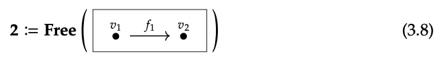
It has two objects \(v_{1}\) and \(v_{2}\), and three morphisms: \(id_{v1}\) : \(v_{1}\) → \(v_{1}\), \(f_{1}\) : \(v_{1}\) → \(v_{2}\), and \(id_{v2}\) : \(v_{2}\) → \(v_{2}\). Here \(id_{v1}\) is the path of length 0 starting and ending at \(v_{1}\), \(f_{1}\) is the path of length 1 consisting of just the arrow \(f_{1}\), and \(id_{v2}\). As our notation suggests, \(id_{v1}\) is the identity morphism for the object \(v_{1}\), and similarly \(id_{v2}\) is the length 0 path at \(v_{2}\).
As our notation suggests, \(id_{v1}\) is the identity morpism for the object \(v_{1}\), and similary \(id_{v2}\) for \(v_{2}\). As composition is given by concatenation, we have, for example \(id_{v1}\) ; \(f_{1}\) = \(f_{1}\), \(id_{v2}\) ; \(id_{v2}\) = \(id_{v2}\), and so on.
From now on, we may elide the difference between a graph and the corresponding free category Free(G), at least when the one we mean is clear enough from context.
For Free(G) to really be a category, we must check that this data we specified obeys the unitality and associativity properties. Check that these are obeyed for any graph G. ♦
The free category on the graph shown here:\(^{4}\)
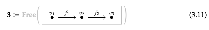
has three objects and six morphisms: the three vertices and six paths in the graph. Create six names, one for each of the six morphisms in 3. Write down a six-by-six table, label the rows and columns by the six names you chose.
- Fill out the table by writing the name of the composite in each cell, when there is a composite.
- Where are the identities? ♦
Let’s make some definitions, based on the pattern above:
- What is the category 1? That is, what are its objects and morphisms?
- What is the category 0?
- What is the formula for the number of morphisms in n for arbitrary n \(\in\) \(\mathbb{N}\)? ♦
Consider the following graph:
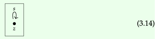
It has only one vertex and one arrow, but it has infinitely many paths. Indeed, it has a unique path of length n for every natural number n \(\in\) N. That is, Path = {z,s,(s ; s),(s ; s ; s),...}, where we write z for the length 0 path on z; it represents the morphism idz . There is a one-to-one correspondence between Path and the natural numbers, N = {0, 1, 2, 3, . . .}.
This is an example of a category with one object. A category with one object is called a monoid, a notion we first discussed in Example 2.6. There we said that a monoid is a tuple (M, ∗, e) where ∗: M × M → M is a function and e \(\in\) M is an element, and m ∗ 1 = m = 1 ∗ m and (m ∗ n) ∗ p = m ∗ (n ∗ p).
The two notions may superficially look different, but it is easy to describe the connection.
Given a category C with one object, say •, let M = C(•, •), let e = \(id_{•}\), and let ∗ : C(•, •) × C(•, •) → C(•, •) be the composition operation ∗ = ;. The associativity and unitality requirements for the monoid will be satisfied because C is a category.
In Example 3.13 we identified the paths of the loop graph (3.14) with numbers n \(\in\) \(\mathbb{N}\). Paths can be concatenated. Given numbers m, n \(\in\) \(\mathbb{N}\), what number corresponds to the concatenation of their associated paths? ♦
Presenting categories via path equations
So for any graph G, there is a free category on G. But we don’t have to stop there: we can add equations between paths in the graph, and still get a category. We are only allowed to equate two paths p and q when they are parallel, meaning they have the same source vertex and the same target vertex.
A finite graph with path equations is called a finite presentation for a category, and the category that results is known as a finitely-presented category. Here are two examples:
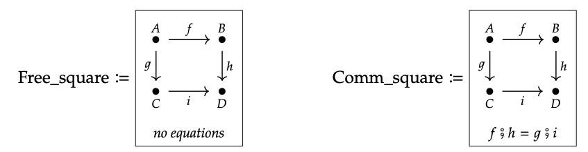
Both of these are presentations of categories: in the left-hand one, there are no equations so it presents a free category, as discussed in Section 3.2.1. The free square category has ten morphisms, because every path is a unique morphism.
- Write down the ten paths in the free square category above.
- Name two different paths that are parallel.
- Name two different paths that are not parallel. ♦
On the other hand, the category presented on the right has only nine morphisms, because f ; h and g ; i are made equal. This category is called the “commutative square.” Its morphisms are
{A, B, C, D, f, g, h, i, f ; h}
One might say “the missing one is g ; i,” but that is not quite right: g ; i is there too, because it is equal to f ; h. As usual, A denotes \(id_{A}\), etc.
Write down all the morphisms in the category presented by the following diagram:
 ♦
♦
We should also be aware that enforcing an equation between two mor- phisms often implies additional equations. Here are two more examples of presentations, in which this phenomenon occurs:
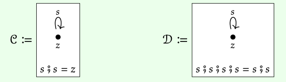
In C we have the equation s ; s = z. But this implies s ; s ; s = z ; s = s ! And similarly we have s ; s ; s ; s = z ; z = z. The set of morphisms in C is in fact merely {z, s}, with composition described by s ; s = z ; z = z, and z ; s = s ; z = s. In group theory, one would speak of a group called \(\mathbb{Z}\)/2\(\mathbb{Z}\).
Write down all the morphisms in the category D from Example 3.18. ♦
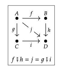
Remark 3.20. We can now see that the schemas in Section 3.1, e.g. Eqs. (3.2) and (3.4) are finite presentations of categories. We will come back to this idea in Section 3.3.
Preorders and free categories: two ends of a spectrum
Now that we have used graphs to depict preorders in Chapter 1 and categories above, one may want to know the relationship between these two uses. The main idea we want to explain now is that
“A preorder is a category where every two parallel arrows are the same.”
Thus any preorder can be regarded as a category, and any category can be somehow “crushed down” into a preorder. Let’s discuss these ideas.
Preorders as categories. Suppose (P, ≤) is a preorder. It specifies a category P as follows. The objects of P are precisely the elements of P; that is, Ob(P) = P. As for morphisms, P has exactly one morphism p → q if p ≤ q and no morphisms p → q if p \(\nleq\) q. The fact that ≤ is reflexive ensures that every object has an identity, and the fact that ≤ is transitive ensures that morphisms can be composed. We call P the category corresponding to the preorder (P, ≤).
In fact, a Hasse diagram for a preorder can be thought of a presentation of a category where, for all vertices p and q, every two paths from p → q are declared equal. For example, in Eq. (1.5) we saw a Hasse diagram that was like the graph on the left:
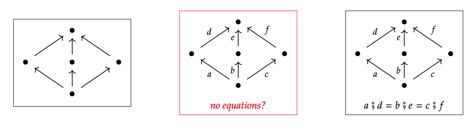
The Hasse diagram (left) might look the most like the free category presentation (middle) which has no equations, but that is not correct. The free category has three morphisms (paths) from bottom object to top object, whereas preorders are categories with at most one morphism between two given objects. Instead, the diagram on the right, with these paths from bottom to top made equal, is the correct presentation for the preorder on the left.
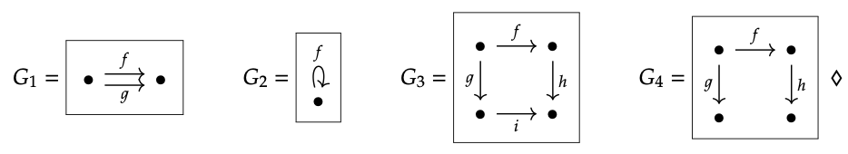
What equations would you need to add to the graphs below in order to present the associated preorders?
The preorder reflection of a category. Given any category C, one can obtain a preorder (C, ≤) from it by destroying the distinction between any two parallel morphisms. That is, let C := Ob(C),and put \(c_{1}\) ≤ \(c_{2}\) iff C( \(c_{1}\), \(c_{2}\)) \(\neq\) Ø. If there is one, or two, or fifty, or infinitely many morphisms \(c_{1}\) → \(c_{2}\) in C, the preorder reflection does not see the difference. But it does see the difference between some morphisms and no morphisms.
What is the preorder reflection of the category \(\mathbb{N}\) from Example 3.13? ♦
We have only discussed adjoint functors between preorders, but soon we will discuss adjoints in general. Here is a statement you might not understand exactly, but it’s true; you can ask a category theory expert about it and they should be able to explain it to you:
Considering a preorder as a category is right adjoint to turning a category into a preorder by preorder reflection.
Remark 3.23 (Ends of a spectrum). The main point of this subsection is that both preorders and free categories are specified by a graph without path equations, but they denote opposite ends of a spectrum. In both cases, the vertices of the graph become the objects of a category and the paths become morphisms. But in the case of free categories, there are no equations so each path becomes a different morphism. In the case of preorders, all parallel paths become the same morphism. Every category presentation, i.e. graph with some equations, lies somewhere in between the free category (no equations) and its preorder reflection (all possible equations).
Important categories in mathematics
We have been talking about category presentations, but there are categories that are best understood directly, not by way of presentations. Recall the definition of category
from Definition 3.6. The most important category in mathematics is the category of sets.
The category of sets, denoted Set, is defined as follows.
(i) Ob(Set) is the collection of all sets.
(ii) If S and T are sets, then Set(S, T) = { f : S → T | f is a function}.
(iii) For each set S, the identity morphism is the function \(id_{S}\) : S → S given by \(id_{S}\)(s) := s for each s \(\in\) S.
(iv) Given f : S → T and g : T → U, their composite is the function f ; g: S → U given by (f ; g)(s) := g(f(s)).
These definitions satisfy the unitality and associativity conditions, so Set is indeed a category.
Closely related is the category FinSet. This is the category whose objects are finite sets and whose morphisms are functions between them.
Let \(\underline{2}\) = {1, 2} and \(\underline{3}\) = {1, 2, 3}. These are objects in the category Set discussed in Definition 3.24. Write down all the elements of the set Set(\(\underline{2}\), \(\underline{3}\)); there should be nine. ♦
Remark 3.26. You may have wondered what categories have to do with V-categories (Definition 2.46); perhaps you think the definitions hardly look alike. Despite the term ‘enriched category’, V-categories are not categories with extra structure. While some sorts of V-categories, such as Bool-categories, i.e. preorders, can naturally be seen as categories, other sorts, such as Cost-categories, cannot.
The reason for the importance of Set is that, if we generalize the definition of enriched category (Definition 2.46), we find that categories in the sense of Definition 3.6 are exactly Set-categories so categories are V-categories for a very special choice of V. We’ll come back to this in Section 4.4.4. For now, we simply remark that just like a deep understanding of the category Cost for example, knowing that it is a quantale yields insight into Lawvere metric spaces, so the study of Set yields insights into categories.
There are many other categories that mathematicians care about:
- Top: the category of topological spaces (neighborhood)
- Grph: the category of graphs (connection)
- Meas: the category of measure spaces (amount)
- Mon: the category of monoids (action)
- Grp: the category of groups (reversible action, symmetry)
- Cat: the category of categories (action in context, structure)
But in fact, this does not at all do justice to the diversity of categories mathematicians think about. They work with whatever category they find fits their purpose at the time, like ‘the category of connected Riemannian manifolds of dimension at most 4’.
Here is one more source of examples: take any category you already have and reverse all its morphisms; the result is again a category.
Let C be a category. Its opposite, denoted \(C^{op}\), is the category with the same objects, Ob(\(C^{op}\)) := Ob(C), and for any two objects c, d \(\in\) Ob(C), one has \(C^{op}\)(c, d) := C(d, c). Identities and composition are as in C.
Isomorphisms in a category
The previous sections have all been about examples of categories: free categories, presented categories, and important categories in math. In this section, we briefly switch gears and talk about an important concept in category theory, namely the concept of isomorphism.
In a category, there is often the idea that two objects are interchangeable. For example, in the category Set, one can exchange the set {∎, □} for the set {0, 1} and everything will be the same, other than the names for the elements. Similarly, if one has a preorder with elements a, b, such that a ≤ b andb ≤ a,i.e.a \(\cong\) b, then a and b are essentially the same. How so? Well they act the same, in that for any other object c, we know that c ≤ a iff c ≤ b, and c ≥ a iff c ≥ b. The notion of isomorphism formalizes this notion of interchangeability.
An isomorphism is a morphism f : A → B such that there exists a morphism g : B → A satisfying f ; g = \(id_{A}\) and g ; f \(id_{B}\). In this case we call f and g inverses, and we often write g = \(f^{−1}\), or equivalently f = \(g^{−1}\). We also say that A and B are isomorphic objects.
The set A := {a, b, c} and the set \(\underline{3}\) = {1, 2, 3} are isomorphic; that is, there exists an isomorphism f: A → \(\underline{3}\) given by f(a) = 2, f(b) = 1, f(c) = 3. The isomorphisms in the category Set are the bijections.
Recall that the cardinality of a finite set is the number of elements in it. This can be understood in terms of isomorphisms in FinSet. Namely, for any finite set A \(\in\) FinSet, its cardinality is the number n \(\in\) \(\mathbb{N}\) such that there exists an isomorphism A \(\cong\) n. Georg Cantor defined the cardinality of any set X to be its isomorphism class, meaning the equivalence class consisting of all sets that are isomorphic to X.
1. What is the inverse \(f^{−1}\) : \(\underline{3}\) → A of the function f given in Example 3.29?
2. How many distinct isomorphisms are there A → \(\underline{3}\)? ♦
Show that in any given category C, for any given object c \(\in\) C, the identity idc is an isomorphism ♦
Recall Examples 3.13 and 3.18. A monoid in which every morphism is an isomorphism is known as a group.
1. Is the monoid in Example 3.13 a group?
2. What about the monoid C in Example 3.18? ♦
Let G be a graph, and let Free(G) be the corresponding free category. Somebody tells you that the only isomorphisms in Free(G) are the identity morphisms. Is that person correct? Why or why not? ♦
In this example, we will see that it is possible for g and f to be almost but not quite inverses, in a certain sense.
Consider the functions f : \(\underline{2}\) → \(\underline{3}\) and g : \(\underline{3}\) → \(\underline{2}\) drawn below:
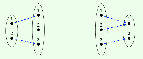
Then the reader should be able to instantly check that f ; g = \(id_{\underline{2}}\) but g ; f \(\neq\) \(id_{\underline{3}}\). Thus f and g are not inverses and hence not isomorphisms. We won’t need this terminology, but category theorists would say that f and g form a retraction.