Southeastern Tropical Atlantic Changing From Subtropical to Tropical Conditions
 Marisa Roch
 Peter Brandt
 Sunke Schmidtko
 Filomena Vaz Velho
 Marek Ostrowski4
- 1GEOMAR Helmholtz Centre for Ocean Research Kiel, Kiel, Germany
- 2Faculty of Mathematics and Natural Sciences, Kiel University, Kiel, Germany
- 3Instituto Nacional de Investigação Pesqueira e Marinha, Luanda, Angola
- 4Oceanography and Climate, Institute of Marine Research, Bergen, Norway
A warming and freshening trend of the mixed layer in the upper southeastern tropical Atlantic Ocean (SETA) is observed by the Argo float array during the time period of 2006–2020. The associated ocean surface density reduction impacts upper-ocean stratification that intensified by more than 30% in the SETA region since 2006. The initial typical subtropical stratification with a surface salinity maximum is shifting to more tropical conditions characterized by warmer and fresher surface waters and a subsurface salinity maximum. During the same period isopycnal surfaces in the upper 200 m are shoaling continuously. Observed wind stress changes reveal that open ocean wind curl-driven upwelling increased, however, partly counteracted by reduced coastal upwelling due to weakened alongshore southerly winds. Weakening southerly winds might be a reason why tropical surface waters spread more southward reaching further into the SETA region. The mixed layer warming and freshening and associated stratification changes might impact the marine ecosystem and pelagic fisheries in the Angolan and northern Namibian upwelling region.
Introduction
The southeastern tropical Atlantic (SETA: 10–20°S, 5°W–15°E) encompasses a highly-productive ecosystem off Angola which is located just north of one of the major global coastal upwelling regions: the Benguela upwelling system (Ostrowski et al., 2009; Kopte et al., 2017). In the SETA region the thermal Angola-Benguela Front (ABF) evolves around 15–17°S where warm, tropical waters encounter cooler, subtropical waters from the Benguela upwelling system (Shannon et al., 1987; Siegfried et al., 2019). At the ABF the poleward Angola Current meets the northward Benguela Coastal Current (Siegfried et al., 2019, indicated schematically in Figure 1a). Siegfried et al. (2019) showed that the Angola Current is fed with tropical South Atlantic Central Water (SACW) via the eastward flowing Equatorial Undercurrent (EUC), the South Equatorial Undercurrent (SEUC) and the South Equatorial Countercurrent (SECC) (Figure 1a). These currents and the location of the ABF undergo large seasonal variations and hence the area influenced by the presence of tropical SACW varies as well (Rouault, 2012).
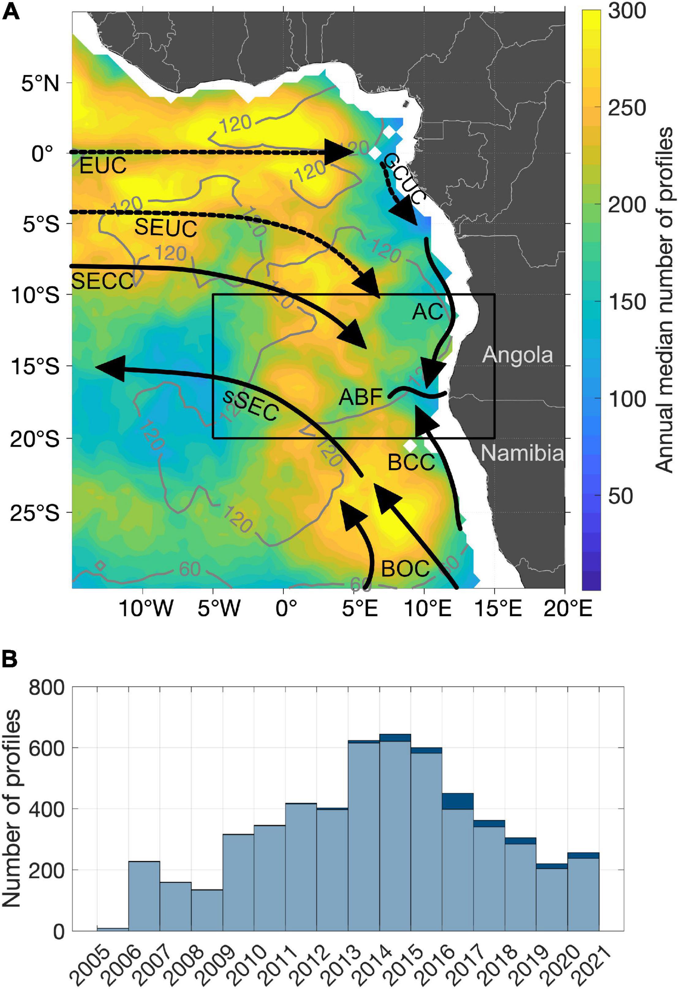
Figure 1. (A) Median annual number of Argo profiles for the time period of 2006–2020. Mapping radii are ellipses with 3° in latitude and 8° in longitude at the equator changing exponentially toward circles with 6° radii in latitude and longitude at 20°S. Gray contour lines show the standard deviation of the median annual number. The black box shows the southeastern tropical Atlantic (SETA) region (10–20°S, 5°W–15°E). Additionally, currents are schematically indicated (solid arrows imply surface currents and dashed arrows thermocline currents): Equatorial Undercurrent (EUC), South Equatorial Undercurrent (SEUC), South Equatorial Countercurrent (SECC), Angola Current (AC), Benguela Coastal Current (BCC), Benguela Oceanic Current (BOC), southern branch of the South Equatorial Current (sSEC), and Gabun-Congo Undercurrent (GCUC). Besides, the location of the Angola-Benguela Front (ABF) is depicted. Shelf regions below 2,000 dbar have been blanked out. (B) Dark blue bars indicate the overall number of Argo profiles in the SETA region per year. Light blue bars above depict the number of Argo profiles that pass the good interquartile range filter of the vertical stratification maximum in the SETA region per year.
On seasonal time scales the variability of the Angola Current is affected by coastally trapped waves (CTWs) excited by remote equatorial forcing (Ostrowski et al., 2009; Bachèlery et al., 2016; Kopte et al., 2018; Tchipalanga et al., 2018). The seasonal upwelling and downwelling phases in the SETA region coincide with the corresponding four seasonal wave propagations of the CTWs. March and October are marked by downwelling and July–August and December-January by upwelling phases (Ostrowski et al., 2009). CTWs excite sea surface temperature (SST) anomalies via the thermocline feedback which can affect air-sea interactions such as heat fluxes and precipitation patterns (Shannon et al., 1986; Rouault et al., 2018).
On top of the seasonal cycle, the SST along the coast of Angola and Namibia can experience extreme warm events, the so-called Benguela Niños (Shannon et al., 1986). During these interannual warm events, the ABF is shifted anomalously poleward (Florenchie et al., 2004; Rouault et al., 2007, 2018; Lübbecke et al., 2010). Thereby, tropical SACW extends into the northern part of the Benguela upwelling region (Lübbecke et al., 2010; Siegfried et al., 2019).
Meteorologically, the SETA region is situated on the northeastern flank of the South Atlantic Subtropical High (SASH) and therefore, the wind pattern is influenced by the southeast trades (Peterson and Stramma, 1991). In the northern part of the SETA region the mainly southerly wind is considerably weak (Risien et al., 2004; Fennel et al., 2012; Lübbecke et al., 2019; Zeng et al., 2021). Besides, in austral winter when SSTs are lowest, the upwelling favorable winds are weakest and thus, the shallowing of the thermocline occurring during that part of the year is not wind-driven. Instead, enhanced biological productivity off Angola in austral winter is mainly associated with the propagation of an upwelling CTW (e.g., Ostrowski et al., 2009; Rouault, 2012; Lübbecke et al., 2019). Mixing dominantly induced by internal tides (Zeng et al., 2021) transfers the CTW upwelling signal toward the surface to further modulate near coastal SST (Imbol Koungue and Brandt, 2021) and transport nutrients upward into the euphotic zone.
In the southern part of the SETA region the wind situation differs as the southerly wind is substantially stronger. This equatorward wind weakens toward the coast and thereby produces a negative wind stress curl which leads to wind curl-driven upwelling, especially off Namibia (Fennel et al., 2012; Lübbecke et al., 2019).
Upwelling is generally considered to be the upward advection forced by Ekman dynamics (via alongshore winds and wind stress curl) and CTWs (Fennel and Lass, 2007; Fennel et al., 2012). CTWs can be generated both locally and thereby partly reducing the effect of local wind-forced upwelling (Fennel and Lass, 2007) or remotely, e.g., by equatorial forcing (Bachèlery et al., 2016). Nutrients that are important for primary productivity can be transported upward by upwelling and mixing, whereas mixing was shown to be particularly effective during upwelling CTW phases (Zeng et al., 2021).
Superimposed on the wide-spread southerly wind component in the SETA region associated with the southeast trades is the atmospheric Benguela low-level coastal jet (BLLCJ, Patricola and Chang, 2017). Low-level coastal jets are marked by strong coast-parallel equatorward winds in eastern boundary upwelling systems. Attributed to the geometry of the coastline, the BLLCJ constitutes of two local maxima in terms of frequency of occurrence around 26 and 17.5°S (Patricola and Chang, 2017; Lima et al., 2019a). The BLLCJ is formed in between the SASH and the Angolan thermal low pressure. The co-existence of these two pressure systems results in strong pressure gradient and forces the equatorward winds (Lima et al., 2019a). According to Patricola and Chang (2017), an intensification of the SASH and a shift toward the African continent strengthens the BLLCJ. The meridional wind stress component is then enhanced in the southern part, but decreasing offshore and to the north of this region.
In the high-productive SETA region both, upwelling and mixing are of great importance for small pelagic fish stocks since upward transport of nutrients directly impact primary production (Ostrowski et al., 2009; Tchipalanga et al., 2018). The extreme warm and frequently occurring Benguela Niños can have dramatic consequences for the marine ecosystem and its productivity. During a major warm event in 1995 e.g., sardinella Sardinella aurita and sardine Sardinops sagax showed a large reduction in biomass with increased mortality in Angolan waters and a southward migration to Namibian coastal waters (Gammelsrød et al., 1998). Besides, Potts et al. (2014) reported an intensified warming over the last three decades with dramatic consequences for some fish species and poleward habitat shifts. For a recent review of the impact of climate variability on the plankton, pelagic and demersal fish communities in the Benguela upwelling system the reader is referred to Jarre et al. (2015). Additionally, Jarre et al. (2015) give an outlook on possible changes of the ecosystem related to climate warming.
In general, upwelling and mixing are affected by upper-ocean stratification. Processes such as ocean ventilation and entrainment into the mixed layer depend on the density gradient at the base of the mixed layer and thus on stratification. In this study, we make use of an extensive Argo float dataset to focus on decadal variability of upper-ocean stratification. Our aim is not to investigate processes on the continental slope and shelf, as the Argo floats cannot represent the shelf region. In particular, we cannot study the effects of Benguela Niños and CTWs by using Argo data. Instead, we focus on larger scale water mass and stratification changes and discuss their possible impact on the marine ecosystem.
The common assumption based on climate projections is that global warming will result in a more stratified ocean due to enhanced warming of the ocean surface, often associated with mixed layer shoaling, reduced ventilation and weaker vertical mixing (Keeling et al., 2010; Capotondi et al., 2012; Rhein et al., 2013). Consequently, less upward nutrient supply to the euphotic zone and declining dissolved oxygen concentration are expected (Capotondi et al., 2012; Ito et al., 2019). Hence, impacts on marine ecosystems can be large. Previous work on upper-ocean stratification has mainly focused on climate models and some of these proposed feedbacks are not that straight forward as many different factors play a role. Ventilation processes for example can be further influenced by changes of the wind-driven circulation and heaving (Huang, 2015). Besides, there can be large regional differences and there are observations indicating deeper mixed layers in regions with enhanced stratification (Somavilla et al., 2017; Sallée et al., 2021). This is counterintuitive and could balance the predicted reduction of vertical mixing. It reveals the general lack of understanding of how physical and biological processes are shifting due to climate warming.
Two recent studies showed increasing global stratification since the 1960s. Yamaguchi and Suga (2019) found a 40% increase of global stratification in the upper 200 m, about half of this enhancement is observed in the tropical oceans. Li et al. (2020) highlight that the global stratification in the upper 2,000 m depth is strengthening by 0.9% per decade (5.3% in total) during the period 1960–2018. Their estimate detects largest stratification increases of 5–18% in the upper 150 m.
When investigating upper-ocean stratification, it is necessary to examine mixed layer properties. Directly below the mixed layer the pycnocline/thermocline representing the vertical stratification maximum is situated. The dynamics of these two components, i.e., the mixed layer and the stratification maximum below, can be linked to each other. However, for the global ocean the evolution of water mass properties at the base of the mixed layer is much less studied than the surface warming (Clément et al., 2020).
The continuous growth of Argo observations in recent years allows us to investigate the tropical Atlantic Ocean in terms of upper-ocean stratification changes, its causes as well as its consequences for physical ocean dynamics and marine ecosystems. In this study we will focus on the SETA region as it encompasses a highly productive ecosystem and hence, investigation of upper-ocean stratification in terms of climate variability in this region is of major economic importance for the Angolan and Namibian fisheries. We aim to provide a better understanding of possible physical changes as a result of climate change and their relation to marine ecosystems.
Data and Methods
Argo Observations and Stratification Estimate
The Argo project currently contains about 4,000 floats measuring hydrographic properties in the upper 2,000 m within a 10-day cycle. For this study Argo observations of the upper 200 m from 2006 to 2019 (Argo, 2019) are used. Prior 2006 the gaps in the data are too large (Roemmich et al., 2015; Desbruyères et al., 2017). Only profiles reaching at least 1000 m depth and flagged good are utilized. The tropical Atlantic from 30°N–30°S holds 121,126 profiles in the observation period. Here, we applied an interquartile range (IQR) filter, excluding data 1.5 times the IQR above/below the first/third quartile. Analyses of potential temperature, absolute salinity and potential density are performed using TEOS-10 (McDougall and Barker, 2011). Additionally, conservative temperature is estimated for the calculation of the Brunt–Väisälä frequency. Note that specifically for the analysis of the SETA region (10°S–20°S, 5°W–15°E) we extended the time series with Argo observations until November 2020, in order to overcome a gap in the data in this particular region in the mid of the year of 2019 (Argo, 2020). The SETA region constitutes 5,477 profiles from 2006 to 2020.
Argo profiles are interpolated vertically using a modified Akima piecewise cubic Hermite interpolation (makima method) as implemented in MATLAB (2019). The algorithm of Akima was first introduced by Akima (1970). Makima is a mixture of the spline and pchip interpolation methods (MathWorks Inc, 2019). Advantages are that makima respects monotonicity compared to the spline method, yet it does not cut off undulations like a pchip method. Using various vertical interpolation schemes, we found that the errors as seen in Supplementary Figure 1B are smallest using the makima method. Furthermore, a linear or piecewise cubic method has maxima and minima centered on measured vertical depth levels. This would lead to a bias using float data, since floats (in particular the ones that transmit the data via ARGOS, as most of them still do) have specific target depth at which they measure the oceanic properties. Thus, for the analysis of vertical maxima and minima using float data, an interpolation scheme that may have local maxima and minima between measurements is necessary and therefore, we chose the makima method. First, all profiles are interpolated on an even 0.01 kg m–3 density grid and second, this is followed by an interpolation on an even 1 dbar pressure grid.
The pressure interpolated profiles are used to determine the Brunt–Väisälä frequency as a measure for stratification. Argo profiles have a varying vertical resolution which impacts the estimate of the Brunt–Väisälä frequency. In order to obtain the best-possible stratification estimate with Argo measurements, we subsampled a high-resolution Conductivity-Temperature-Depth (CTD) profile from a recent cruise in the equatorial Atlantic (Meteor cruise M158, Brandt et al., 2021) onto the vertical resolution of all available Argo profiles for this study. The CTD profile was taken at 0°, 11°W in October 2019 and covers a vertical sampling rate of 1 dbar. The above explained makima interpolation method was applied to the temperature and salinity profiles subsampled according to the vertical resolution of measured Argo profiles. In a next step the Brunt–Väisälä frequency was computed on the even pressure grid. With this we derived a large amount of artificial Argo profiles which are based on the same Brunt–Väisälä frequency profile. However, they deviate from each other since they are based on different vertical resolutions. Finally, the vertical maximum in the upper 200 m of the water column was determined.
By assuming the CTD vertical stratification maximum being the “true” value, we analyzed the dependence of the vertical stratification maximum on the vertical sampling rate of the Argo profiles. The deviations are large (Supplementary Figure 1). However, by using the above described IQR filter and a 15-dbar window for computations, the errors were largely reduced (Supplementary Figure 1). This smoothing length scale was done by trial and error always in comparison to the CTD reference value. In addition, this smoothing length scale is required for the study of background stratification, ignoring other small-scale features that influence the stratification. 15-dbar seems to be the ideal range for this study as it is the balance between minimizing the noise and preserving the shape of the stratification profile (Feucher, 2016).
Mixed layer properties are determined by using the algorithm by Holte and Talley (2009). This algorithm is based on a hybrid method which combines threshold and gradient methods to specify the best mixed layer properties (Holte and Talley, 2009).
Mapping is accomplished using a least squares method which takes the uneven distribution of Argo profiles into account. Despite generally fewer profiles in the South Atlantic (Figure 1a), the histogram of the SETA region indicates more than 300 profiles per year from 2009 to 2018. Influence radii of the anomalies of stratification and mixed layer properties have been checked with a semivariogram analysis, in order to evaluate the spatial bias. This yielded that the spatial bias of the profiles in the SETA region is generally small. Results from 2006 to 2008 and from mid 2019 should be taken with caution due to the relatively small number of Argo profiles available (Figure 1b). The histogram also shows the number of profiles per year that pass the IQR filter for the vertical stratification maximum (Figure 1b). From those 5,477 available profiles in the SETA region 5,297 profiles pass the IQR filter.
Trends and time series of Argo observations are always computed from anomalies relative to the seasonal mean. Seasonal means are calculated on a 15-day grid resolution using overlapping 3-month means (i.e., ±45 days). In order to test statistical significance of the trends, the 95% confidence limits were determined by multiplying the t-value of the Student’s t distribution for 95% significance with the standard error of the trend. In case the slopes of the upper and lower confidence limits are of the same sign, the trend is assigned to be of 95% statistical significance.
Wind Stress Data
To investigate changes of wind speed, zonal and meridional wind stress components the wind product Global Ocean Wind L4 Reprocessed Monthly Mean Observations from Copernicus Marine environment monitoring service (CMEMS) is used (Wind TAC, 2018). The measurements are based on ASCAT scatterometers on METOP-A and METOP-B satellites with the processing level L4. This product is composed of three different ASCAT products (Bentamy, 2020) spanning the global ocean with a spatial resolution of 0.25° × 0.25°. It encompasses monthly means which are estimated from at least 25 daily values at each grid point (Bentamy and Fillon, 2012). The observation period covers May 2007–December 2019. With the meridional and zonal wind stress components, the wind stress curl is computed as well. To reduce noise, the data has been transformed on a 0.5° × 0.5° horizontal grid by taking the mean of all points within ±2° in longitudinal and latitudinal direction around each grid point. The anomalies of the wind data are evaluated by subtracting the monthly means provided by CMEMS from the time series.
Heat Flux and Freshwater Products
In order to compare the results to heat and freshwater fluxes different products are used. First of all, the Objectively Analyzed air-sea fluxes (OAFlux) for the Global Oceans from Woods Hole Oceanographic Institution (WHOI) is used1 (Yu et al., 2008). The horizontal resolution of the data is 1° × 1° in latitude and longitude and is available as a monthly mean from 1958 until present. OAFlux latent and sensible heat fluxes are computed with the COARE bulk flux algorithm and surface meteorological properties (Yu et al., 2008). For this analysis, latent heat flux, evaporation and specific humidity are used for the time period of 2006–2019.
In addition, TropFlux latent heat flux and specific humidity are compared to OAFlux data (Praveen Kumar et al., 2012). TropFlux heat fluxes are calculated from the COARE v3 algorithm. In contrast to OAFlux, TropFlux uses ERA-I and therefore, the two datasets are to some extent not related to each other (Praveen Kumar et al., 2012). According to Praveen Kumar et al. (2012), TropFlux and OAFlux are the best-performing heat flux products. TropFlux horizontal resolution is identical to OAFlux, the monthly estimates from 2006 to 2018 are used.
Furthermore, monthly precipitation estimates from the Global Precipitation Climatology Project (GPCP) Version 2.3 are analyzed (Adler et al., 2018; Pendergrass et al., 2020). This data set has a horizontal resolution of 2.5° × 2.5° and data from 2006 to 2019 is used. GPCP combines several satellite measurements and gauge data.
Similar as for the wind data, the heat flux, evaporation and precipitation data are available as monthly estimates. Anomalies are computed by subtracting the corresponding monthly climatology. Finally, with these anomalies the linear decadal trends are computed.
Net Primary Production
Stratification changes are compared to net primary production data from the Ocean Productivity site2 (Behrenfeld and Falkowski, 1997). The data is based on the Eppley Vertically Generalized Production Model (VGPM) which uses MODIS chlorophyll, SST data, SeaWiFs PAR and estimates of the euphotic zone depth. Net primary production is available for the period of 2002–2019 as monthly values and this study focusses on the years 2006–2019. The horizontal resolution is 1/6° in latitude and longitude but the net primary production was re-gridded on a 0.5° × 0.5° spatial grid to reduce noise.
Theoretical Background
Pure Warming and Freshening Processes in Terms of Heave and Spice
To investigate possible causes for stratification changes it is important to understand that depending on the mean temperature and salinity distribution different processes can dominate. The most common cause for increasing upper-ocean stratification is surface warming, i.e., surface density reduction. Surface warming can be explored in terms of a vector summation between heave and spice (Bindoff and McDougall, 1994; Häkkinen et al., 2016). However, the sign of heave and spice depends strongly on the stability ratio in the region.
The SETA region encompasses a typical subtropical stratification, i.e., warm and saline water layered above cool and fresh water. Then a pure warming or pure freshening process (i.e., a density reduction) at a fixed depth can be interpreted by using a T-S diagram as follows: in case of a pure warming process (Figure 2A, orange arrow) the original thermocline (thin blue line) is shifted to a new position (thick blue line). This results into positive heaving, i.e., the original density surface is sinking downward and is replaced by a lower density on top. This heaving is then corrected by a negative spice contribution which is the temperature and salinity change on a density surface. Thus, a parcel at position 2 appears now cooler and fresher than a parcel at position 3 at the same density on the original thermocline (Figure 2, following Bindoff and McDougall, 1994; Häkkinen et al., 2016).
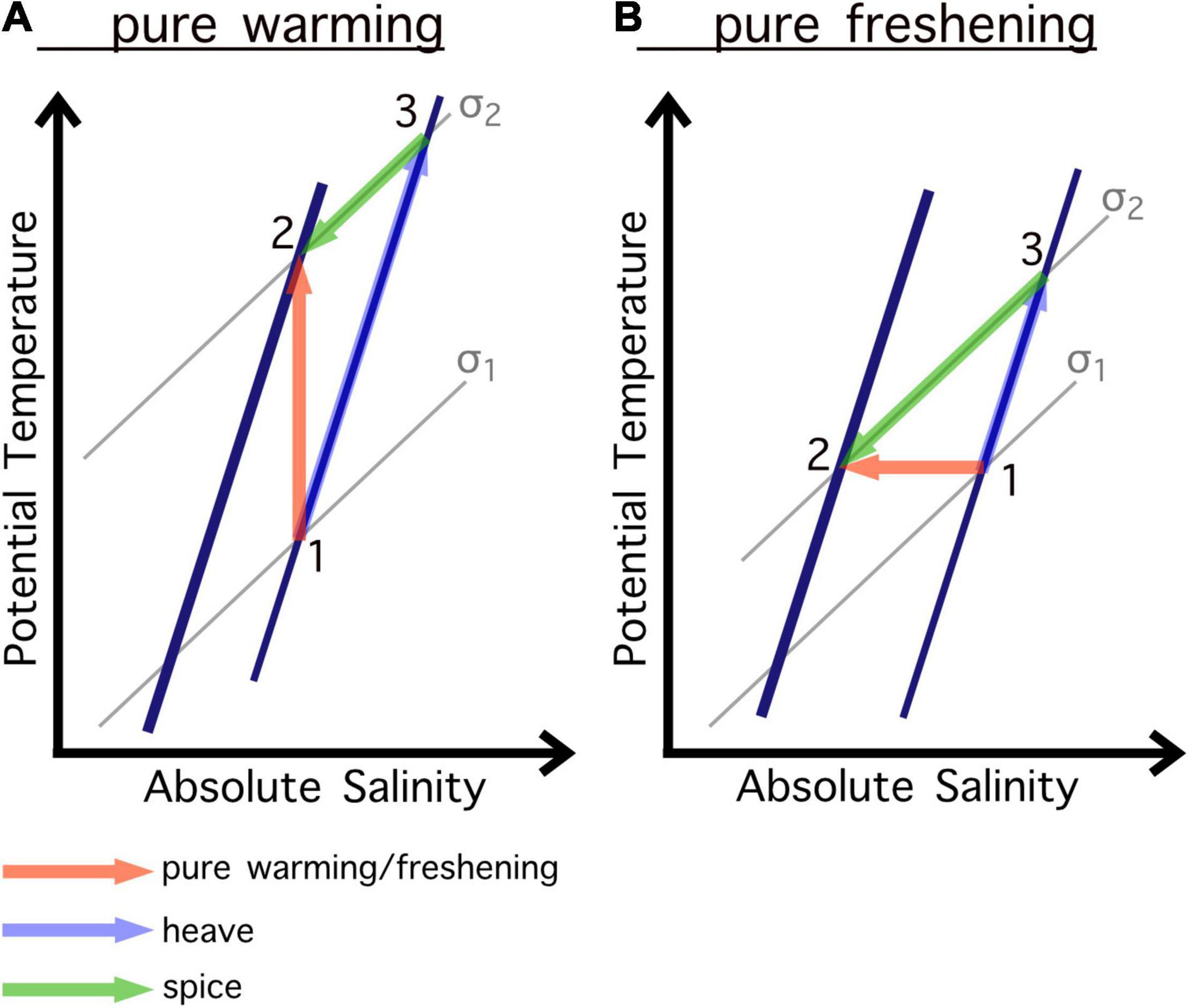
Figure 2. T-S relation schematic for a pure warming process (A) and a pure freshening process (B) for a subtropical stratification (adapted from Bindoff and McDougall, 1994; Häkkinen et al., 2016). Thin blue line indicates initial thermocline, thick blue line the new thermocline. Gray lines show the potential density surfaces (σ1 as the initial density surface and σ2 as the density surface at the same depth after the warming/freshening process with σ2 being smaller and thus lighter than σ1). 1 indicates the initial starting point, 2 reveals the T-S condition at the same depth after warming/freshening. Orange arrows (1–2) denote the warming/freshening process, green arrows indicate the spice component (3–2) and blue arrows the heave component (1–3).
The same processes are active for a pure freshening (Figure 2B). Instead, a cooling or salinification at a fixed depth results in negative heave and positive spice, i.e., an upward displacement of the isopycnals and warm/saline conditions on the initial density surface (not shown). Note the described cases above are the simplest ones. Observed water mass changes will always be a combination of both.
Pure Heaving Process
Another process that can influence the vertical stratification is pure heaving, e.g., due to changes of wind stress curl. This mechanism is not associated with imprints in the T-S diagram (Bindoff and McDougall, 1994). If wind stress curl-driven upwelling intensifies, isopycnals will rise upward and thereby reducing the height difference between near-surface isopycnals (Figure 3) and correspondingly increasing the near-surface stratification or Brunt–Väisälä frequency. In case the height difference between isopycnals is increasing, the stratification decreases. Heaving can thereby alter vertical stratification and additionally may lead to shifts in the heat content (Huang, 2015).
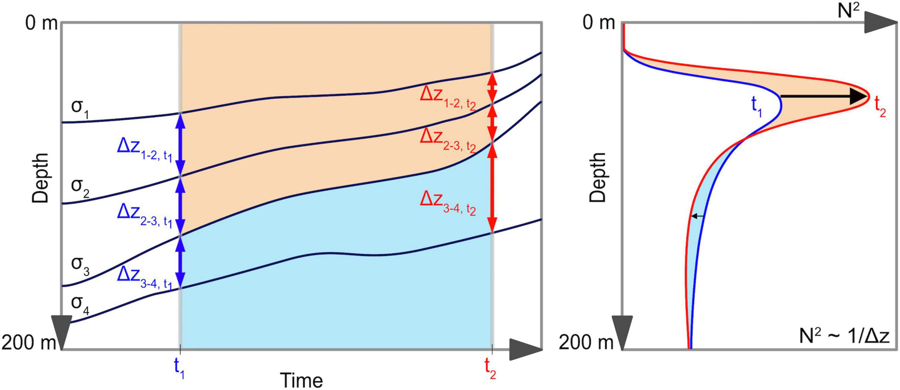
Figure 3. Schematic of a pure heaving process as a result of intensified wind curl-driven upwelling. Dark blue lines indicate different isopycnals (σ1, σ2, σ3, and σ4) whose depth is changing over time. Due to the upwelling of the isopycnals, the height difference Δz between two isopycnals changes over time (compare time steps t1 and t2). If the Δz decreases as for the upper two pairs of isopycnals (Δz1–2, Δz2–3) from time step t1 (blue double arrows) to t2 (red double arrows), the stratification in terms of the Brunt–Väisälä frequency N2 increases as indicated in the right panel by the typical stratification profile. Here the blue line of the N2 profile corresponds to the time step t1 as in the left panel. The red profile indicates the profile for t2. In both panels the depth range where stratification increases, is shaded light orange. In contrast, if the height difference becomes larger over time as for the lower pair of isopycnals (Δz3–4), stratification will be reduced. The depth range where stratification decreases is marked light blue in both panels.
Results
Decadal Trends of the Tropical Atlantic
This section will deal with mean fields and decadal trend maps of vertical stratification maximum, its depth, mixed layer properties, the vertical displacement and spice of isopycnals in the tropical Atlantic. In order to receive an overview about the on-going changes and explain why we particularly focus on the SETA region (10–20°S, 5°W–15°E) for a more detailed analysis, the maps of the vertical stratification maximum and its depth are computed for the entire tropical Atlantic from 30°N to 30°S. All other maps are confined to a smaller region in the eastern tropical Atlantic ranging from 10°N–30°S, 15°W–20°E which includes the SETA region and is still large enough to explain some observed larger-scale patterns.
The vertical stratification maximum is located just below the mixed layer and is within the depth range of the thermocline. The mean of the vertical stratification maxima shows largest values within 10°N and 10°S especially close to the eastern boundary (Figure 4A). These areas largely coincide with areas where the mean depth of the stratification maximum is shallowest (Figure 4B).
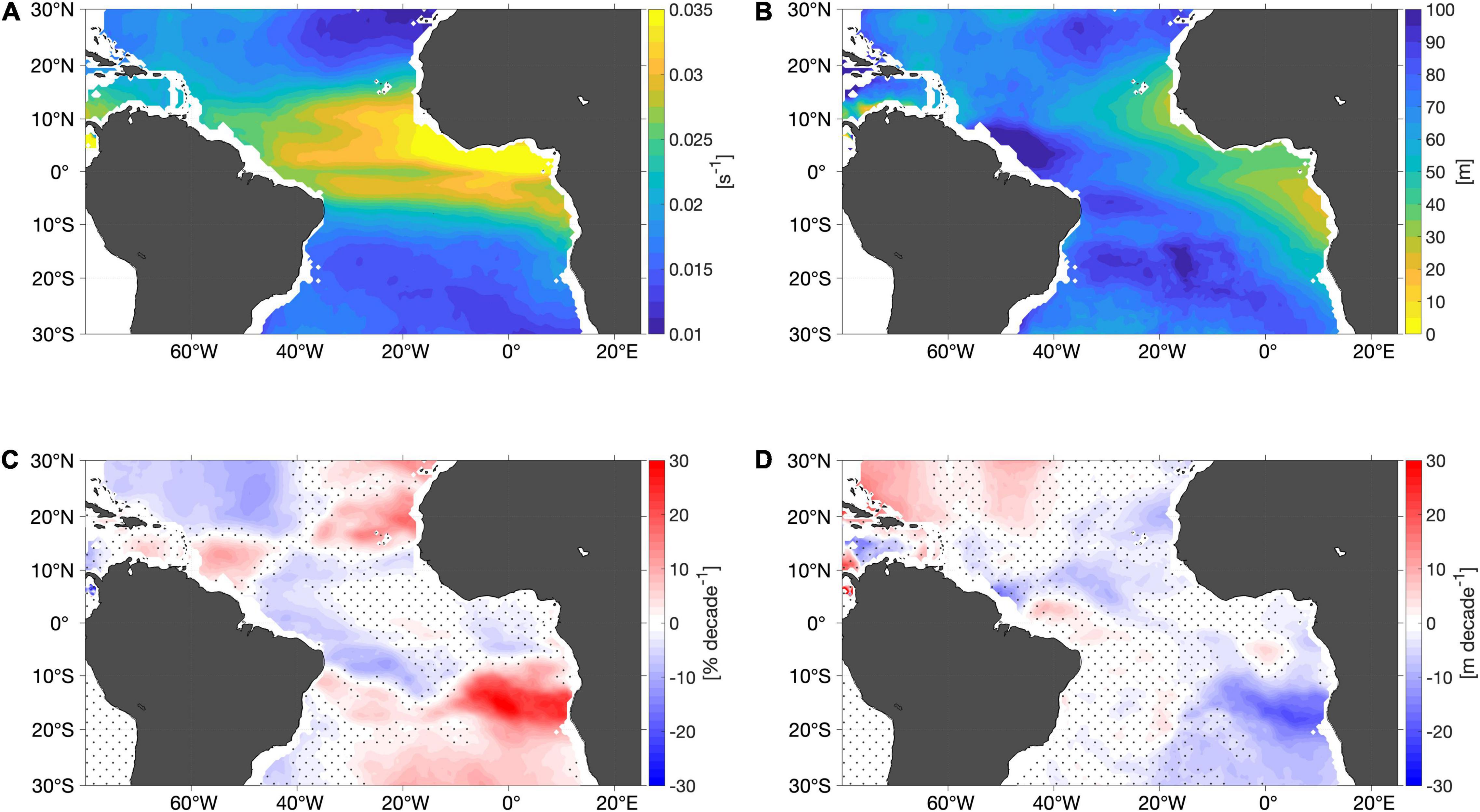
Figure 4. (A) Mean of vertical stratification maxima inferred from Argo for the time period of 2006–2019. (B) Mean depth of the vertical stratification maximum from (A). Panels (C,D) decadal trend of (A,B), respectively. Trends are computed from the anomalies relative to the seasonal mean. Please note, positive trend of depth refers to a deepening. Areas where the trend is not of 95% significance are stippled. Shelf regions below 2,000 dbar are blanked out.
The decadal trend reveals an increase of stratification in the eastern tropical North Atlantic and in most of the tropical South Atlantic away from the equatorial band with maximum increase in the region of SETA (10–20°S, 5°W–15°E) with an intensification of up to 30% (Figure 4C). Besides, where the stratification maximum intensifies, its depth is shoaling (Figure 4D). The described increase of stratification in the SETA region as well as in the northeastern tropical Atlantic (Figure 4C) are of 95% statistical significance.
To better characterize the above results, decadal trends of surface mixed layer characteristics have been calculated for the smaller region in the eastern tropical Atlantic (10°N–30°S, 15°W–20°E) (Figure 5). On average, the MLD can be found only slightly above the vertical stratification maximum. The equatorial region reveals a deepening of the mixed layer, a cooling and salinification and thus, an increase in density. Further south in the SETA region the MLT is rising, MLS is reducing and the MLD is shoaling (Figure 5). Indeed, at the depth of the vertical stratification maximum the patterns of temperature, salinity and density changes are similar (not shown).
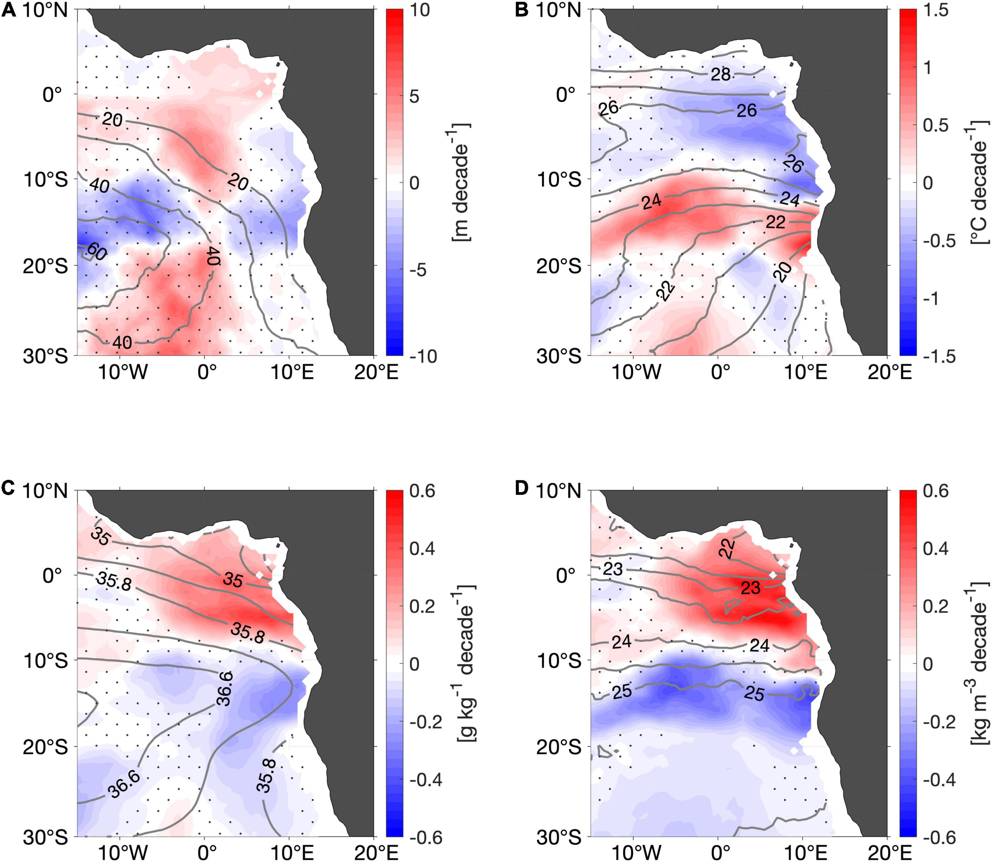
Figure 5. Decadal trend of (A) mixed layer depth (MLD), (B) mixed layer temperature (MLT), (C) mixed layer salinity (MLS), and (D) mixed layer potential density anomalies from Argo for the time period of 2006–2019. Trends are computed from the anomalies relative to the seasonal mean. Mixed layer properties have been estimated with the Holte and Talley algorithm (Holte and Talley, 2009). Gray contour lines show the mean fields for the period of 2006–2019, respectively. Areas where the trend is not of 95% significance are stippled. Please note, positive trend of MLD refers to a deepening of the mixed layer. Shelf regions below 2,000 dbar are blanked out.
In order to understand the acting processes, it is important to not only investigate changes on depth levels but also on density surfaces. Therefore, we inspect the trends of the vertical displacement (i.e., heave) and the spice of two different isopycnals (25.5 and 26.0 kg m–3). These isopycnals are chosen as they are surrounding the vertical stratification maximum in the SETA region. The results of the decadal heave trend show that in most of the southeastern tropical Atlantic these two isopycnals, lying within the upper 150 m, are shoaling (Figures 6A,B). The strongest upwelling of the isopycnals is within 10° offshore in the SETA region whereas there is weaker upwelling along the coast (Figures 6A,B). Spice trends are relatively weak with a range of up to ±0.2 g kg–1 decade–1 (Figures 6C,D). Nevertheless, from the African coastline to 5°W–0° the spice is reducing. Westward of the Greenwich meridian the spice trend is increasing (Figures 6C,D).
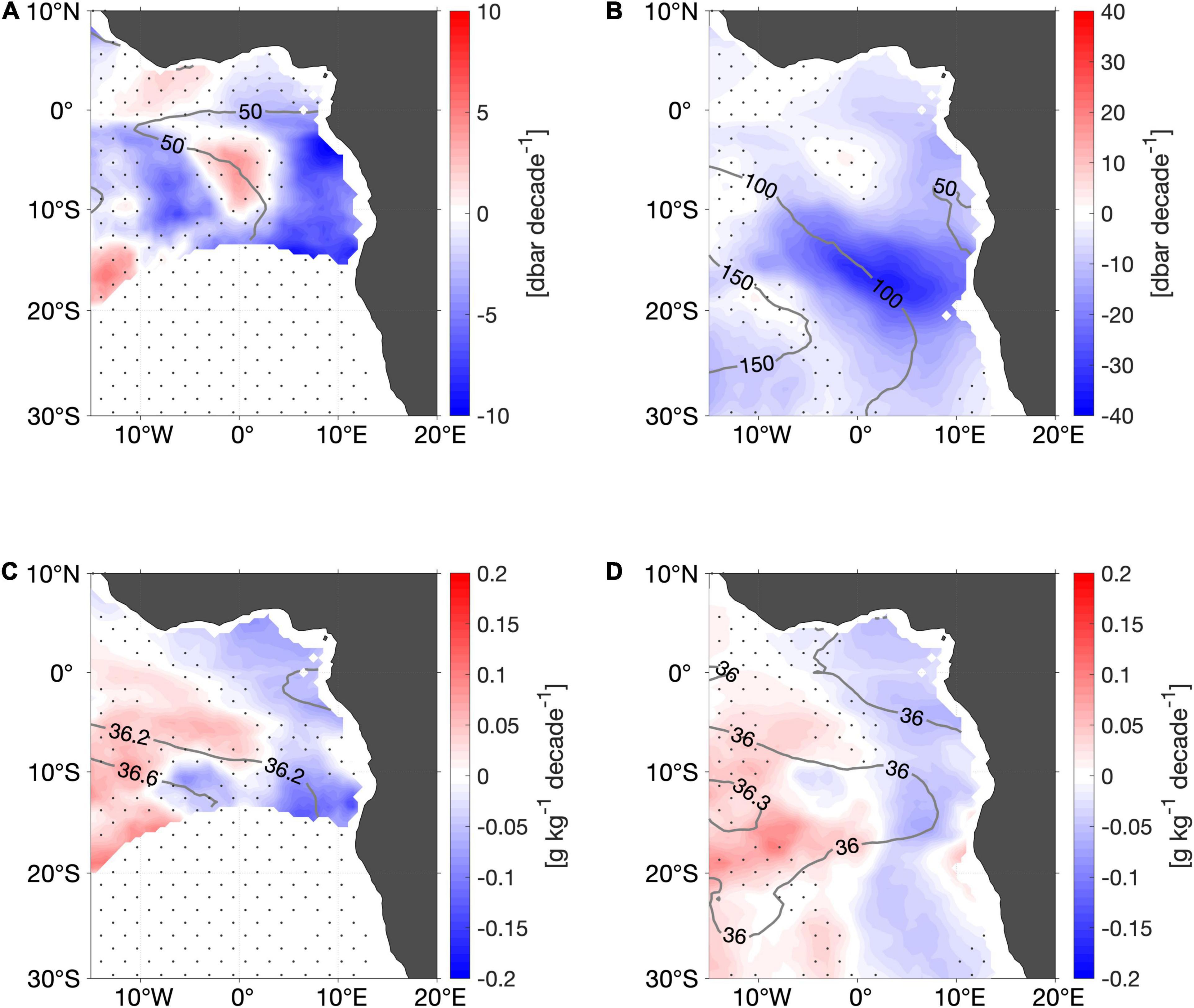
Figure 6. Decadal trend of pressure of the isopycnal surfaces (A) 25.5 kg m–3 and (B) 26.0 kg m–3 and decadal trend of absolute salinity on the isopycnal surfaces (C) 25.5 kg m–3 and (D) 26.0 kg m–3 from Argo for the time period of 2006–2019. Trends are computed from the anomalies relative to the seasonal mean. Gray contour lines show the mean fields on each isopycnal surface for the time period of 2006–2019. Areas where the trend is not of 95% significance are stippled. Please note, positive trend of pressure of isopycnals surfaces refers to a deepening of the isopycnals. Shelf regions below 2,000 dbar are blanked out.
Regional Analysis of Southeastern Tropical Atlantic Ocean Region
In this section the SETA region (10–20°S, 5°W–15°E) is investigated in more detail by analyzing its time series. SETA is the region which undergoes the largest stratification increase within the entire tropical Atlantic during the Argo period.
In fact, the 6 months running median time series of the percental change of the stratification maximum confirms the observed decadal trend in the SETA region as it continuously intensifies. From 2006 to 2016 the stratification increased by 40% (Figure 7A). From 2016 until the beginning of 2020 the stratification intensified by almost another 20%. The time series of the depth anomaly onto the mean depth of the stratification maximum shows that the depth is indeed shoaling (around 50 m from 2006 to 2020, Figure 7B). The same accounts for the MLD which is on average 20–40 m above the depth of the vertical stratification maximum (Figure 7B).
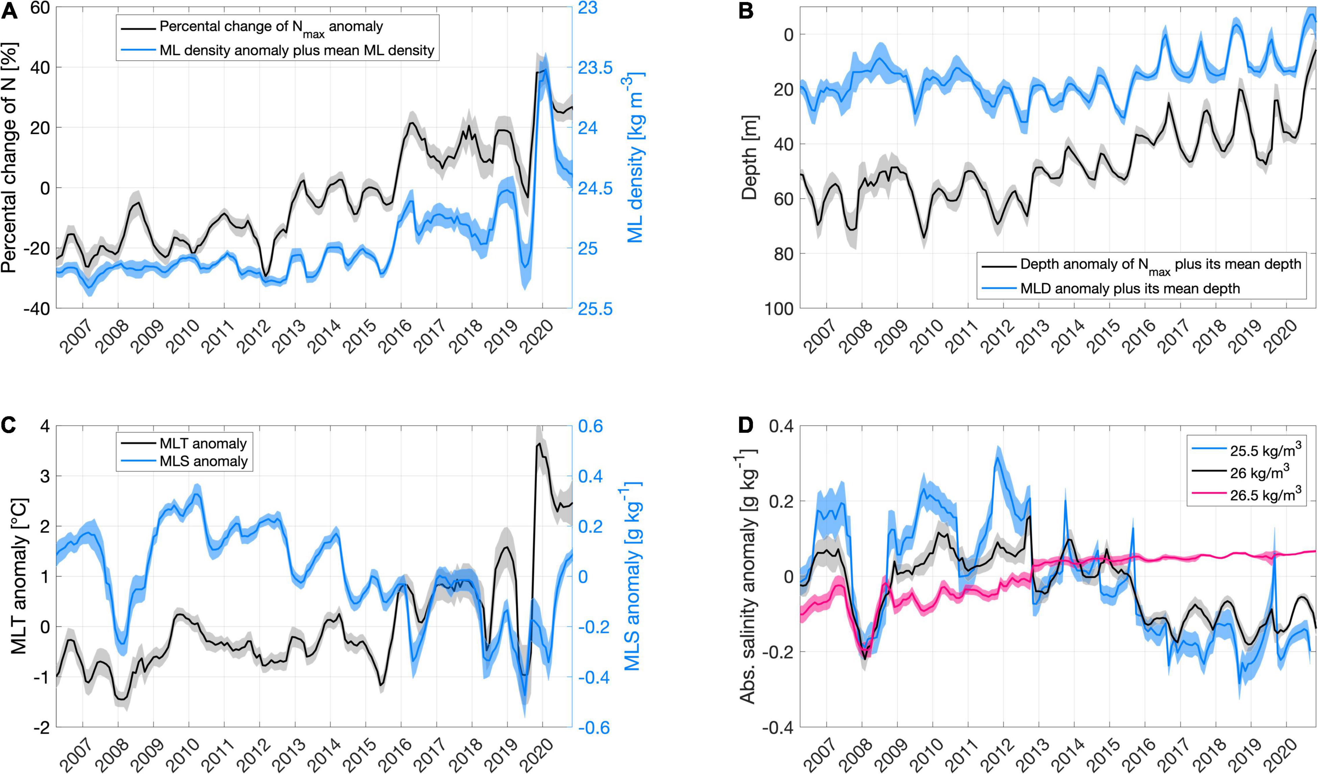
Figure 7. Six months running median of (A) percental change of stratification anomaly of its vertical maximum Nmax (black line, left y-axis) and mixed layer (ML) density anomaly plus mean ML density (blue line, right y-axis), (B) depth anomaly of the vertical stratification maximum plus its mean depth (black line, left y-axis) and mixed layer depth (MLD) anomaly plus mean MLD (blue line, right y-axis), (C) mixed layer temperature (MLT) anomaly (black line, left y-axis) and mixed layer salinity (MLS) anomaly (blue line, right y-axis) and (D) salinity anomaly on the isopycnal surfaces (i.e., spice anomaly) in SETA (10–20°S, 5°W–15°E). In (D) blue line denotes the 25.5 kg m–3 isopycnal, black line the 26.0 kg m–3 isopycnal and pink line the 26.5 kg m–3 isopycnal. All anomalies are computed relative to the seasonal mean. Shading shows the corresponding 95% confidence interval.
The time series of MLT anomaly reveals almost 3°C temperature rise in the SETA region from 2006 to 2018 (Figure 7C). This temperature increase is followed by a minimum of almost −1°C in mid of 2019. At the end of 2019 and beginning of 2020 the MLT depicts a large maximum by around 3.5°C which is by far the greatest peak of the MLT timeseries. MLS is decreasing over time (more than 0.5 g kg–1), however, there is a negative peak in 2008 (Figure 7C). Thus, as the mixed layer is becoming warmer and fresher, the density is decreasing (Figure 7A). The warming and freshening can be found at the depth of the vertical stratification maximum as well even though not as pronounced as in the mixed layer (not shown).
Shown as well are the time series of salinity anomalies on the isopycnals 25.5, 26.0, and 26.5 kg m–3 (spice anomalies). The pattern of the time series of spice changes along the 25.5 and 26.0 kg m–3 isopycnal surfaces is similar to that of MLS (Figure 7D). We observe the negative peak in 2008 and since 2011 the spice is decreasing. The spice on the 26.5 kg m–3 isopycnal is increasing over time indicating that at larger depths different processes are active.
In order to visualize salinity, temperature and stratification changes within the upper 200 m of the water column in the SETA region, a T-S diagram for annual averages of the Argo temperature and salinity profiles was drawn (Figure 8). The derived T-S diagram highlights a typical subtropical stratification with warm, saline water layered above cool, fresh water on average in the SETA region. The annual mean profiles indicate that the water column becomes more stratified during the observing period (Figure 8). However, this does not happen constantly on all depth levels. Largest changes are indeed found in the near-surface waters where the conditions are changing toward warmer and especially fresher characteristics. This confirms the observed mixed layer changes. Since 2009 this shift happens to be continuous and thus, the upper water column is becoming more stratified (Figure 8).
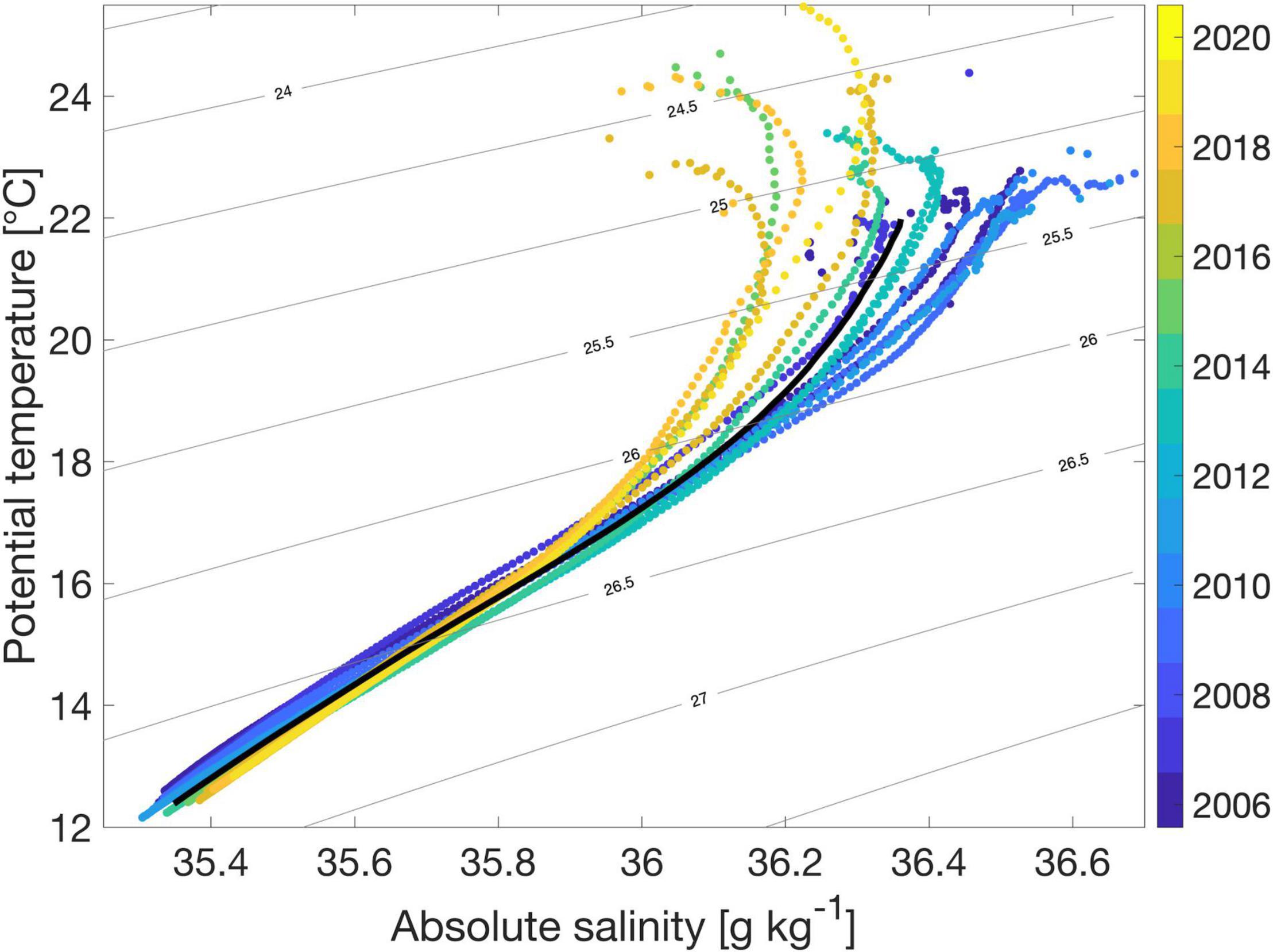
Figure 8. T-S diagram of annual mean potential temperature and absolute salinity values of the upper 200 m in the SETA region (10–20°S, 5°W–15°E). Black line indicates the mean of the time period of 2006–2020.
The T-S diagram reveals that in deeper levels the stratification is becoming slightly weaker (Figure 8). This is supported by mean Brunt–Väisälä frequency profiles for three time periods: 2006–2010, 2011–2015, and 2016–2020 which indicate a continuous increase of stratification in the upper 60 dbar and a decrease below 60 dbar (Figure 9B). In comparison to the stratification profiles, the time series of the 6 months running median pressure anomaly of the three isopycnal surfaces 25.5, 26.0, and 26.5 kg m–3 plus their corresponding mean pressure are shown. We can see how the isopycnals change their vertical position and how the stratification profile alters in the respective depth over the corresponding time period (Figure 9A). The time series indicate a steady upward displacement of the three isopycnals. However, the height difference between the isopycnals changes differently (Figure 9A). This is especially visible from the slope of the corresponding trend lines (Figure 9A). We find that in the depth range of the largest stratification increase, the isopycnals surfaces 25.5 and 26.0 kg m–3 are becoming closer to each other. Whereas below, the height difference between the 26.0 and the 26.5 kg m–3 enlarges. This is the same depth range where stratification weakens.
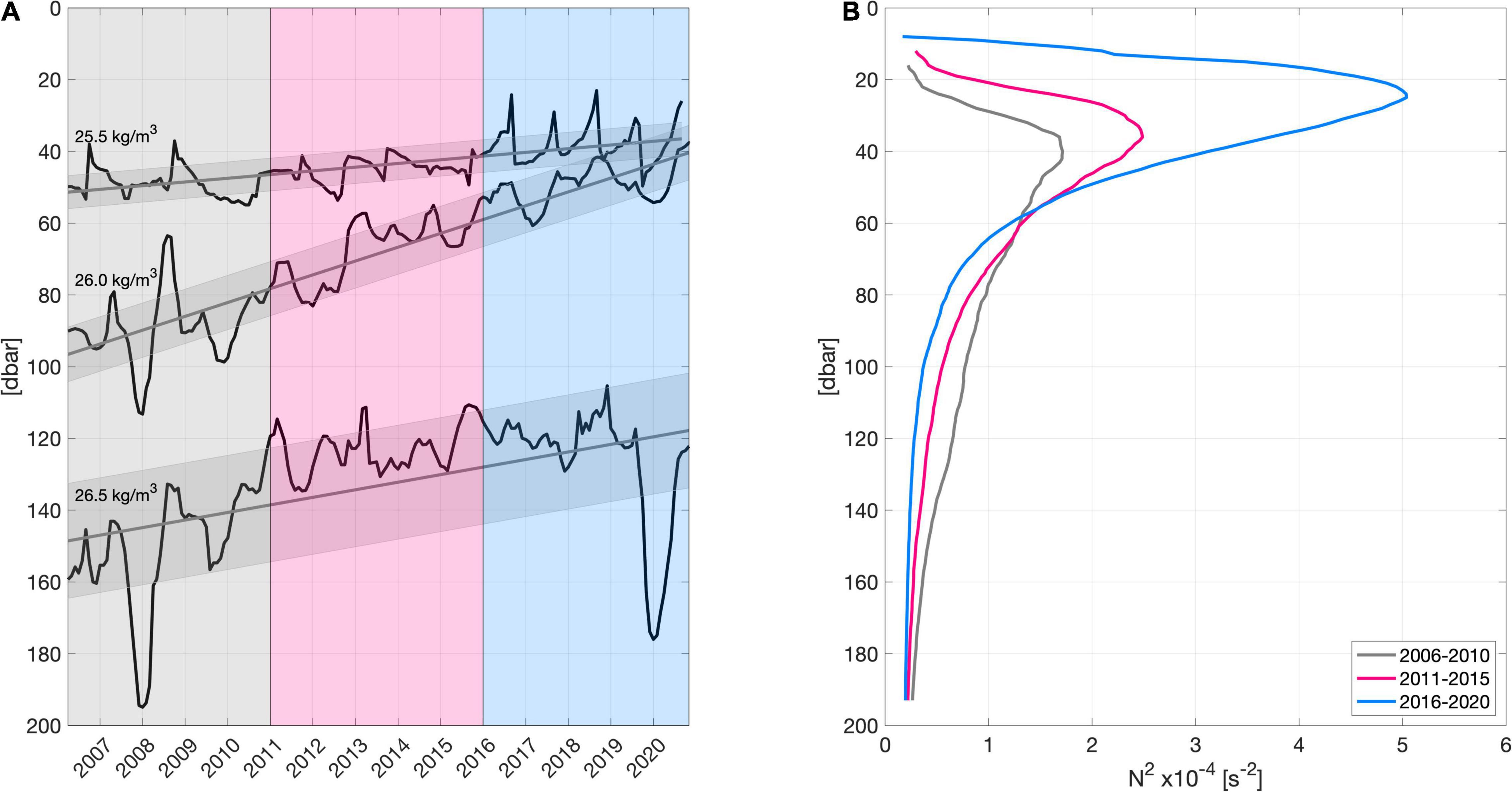
Figure 9. (A) Six months running median pressure anomaly of three isopycnals (25.5, 26.0, and 26.5 kg m–3) plus their corresponding mean pressure in the SETA region (10–20°S, 5°W–15°E). For each isopycnal the linear trend (gray line) and its standard error are shown (gray shading around the linear trend lines). Shaded areas indicate the time periods for the corresponding mean Brunt–Väisälä frequency profile of the upper 200 dbar in (B). Gray shows the mean for the time of 2006–2010, pink denotes the mean of 2011–2015 and blue indicates the period of 2016–2020.
Decadal Wind Stress Changes in Southeastern Tropical Atlantic Ocean Region
In this section we contrast the prior findings of the decadal changes in the SETA region with changes of the wind stress curl, zonal and meridional wind stress components as well as wind speed. Starting with the decadal trend maps of these four variables in the eastern tropical Atlantic to achieve an overview (Figure 10), we discover that close to the African coast in the South Atlantic east of the mean zero-line, the wind stress curl reveals a negative trend. This implies the wind stress curl in this region is becoming more negative. West of the zero-line the wind stress curl anomaly shows a positive trend (Figure 10A).
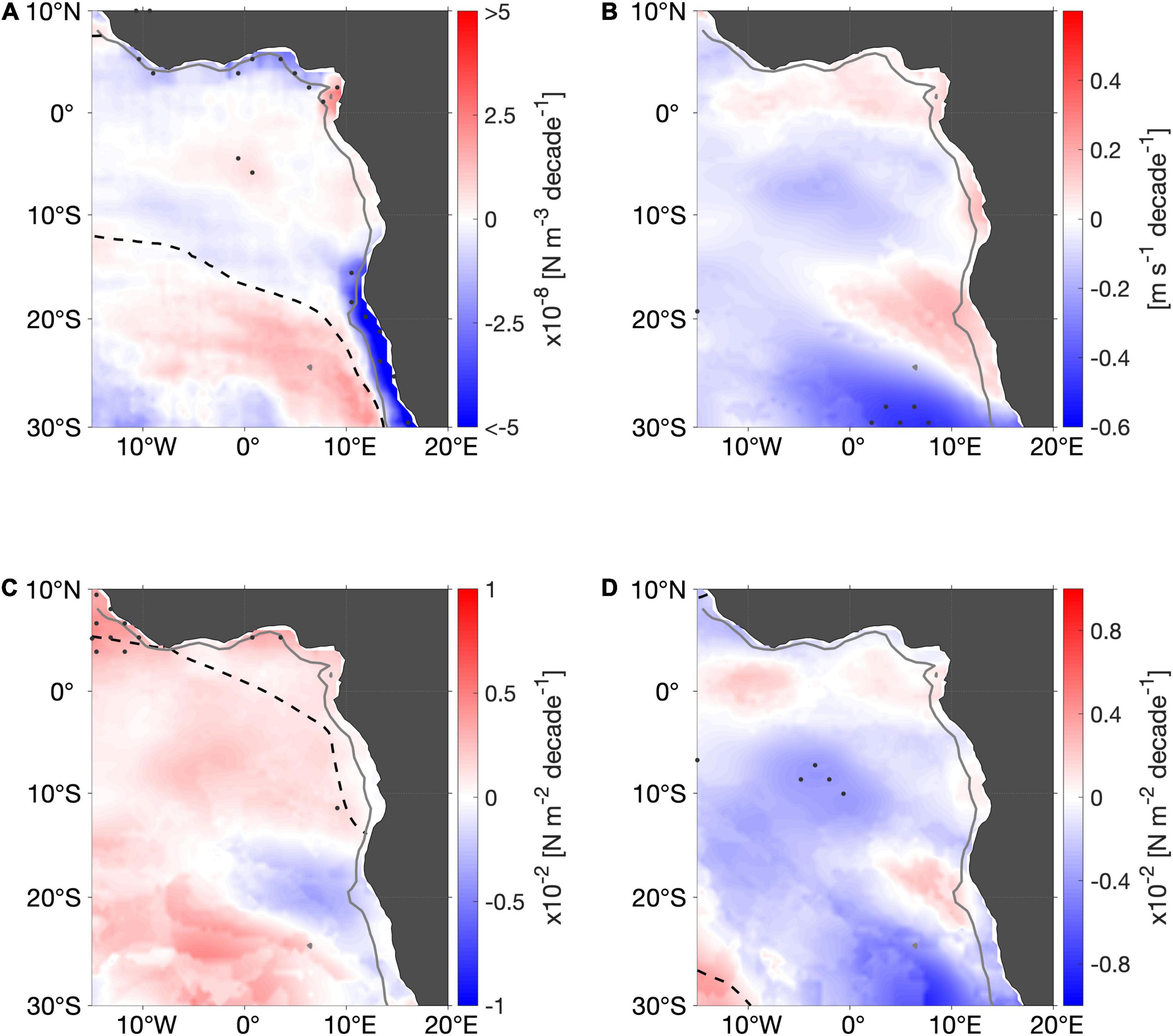
Figure 10. Decadal trend of (A) wind stress curl, (B) wind speed, (C) zonal wind stress component, and (D) meridional wind stress component from monthly values from Copernicus Marine environment monitoring service (CMEMS) from ASCAT scatterometers on METOP-A and METOP-B satellites for the time period of 2007–2019. Trends are computed from the anomaly relative to the monthly mean. Black dashed lines indicate the zero-lines of the corresponding mean fields, respectively. Areas where the trend is of 95% significance are stippled. Gray line marks the 2,000 dbar isobath of the shelf regions.
The decadal trend of the wind speed anomaly shows an increase in the southern part of SETA, whereas in the northern part of SETA and around SETA the trend of wind speed is negative (Figure 10B). Comparing this to the zonal wind stress component, we find a negative trend in the area of intensified wind speed in SETA, i.e., intensified easterlies. The positive trend is surrounded by westerly trend. The meridional wind stress component which is on average directed northward in the SETA region depicts a negative trend in the northern part of this region, thus, indicating a weakening of southerly winds. In the southern part of SETA, the wind stress anomaly shows a slight increase of the northward component (Figure 10D).
Focusing on the wind stress curl and the meridional wind stress component, the zonal sections of the 6 months running mean of the two components in the SETA region, show that indeed within 500 km of the coast the wind stress curl becomes more negative. In contrast, since 2009 meridional wind stress anomalies shift from northward to southward anomalies within about 200 km of the coast. Since 2017 again more northward anomalies are observed (Figure 11).
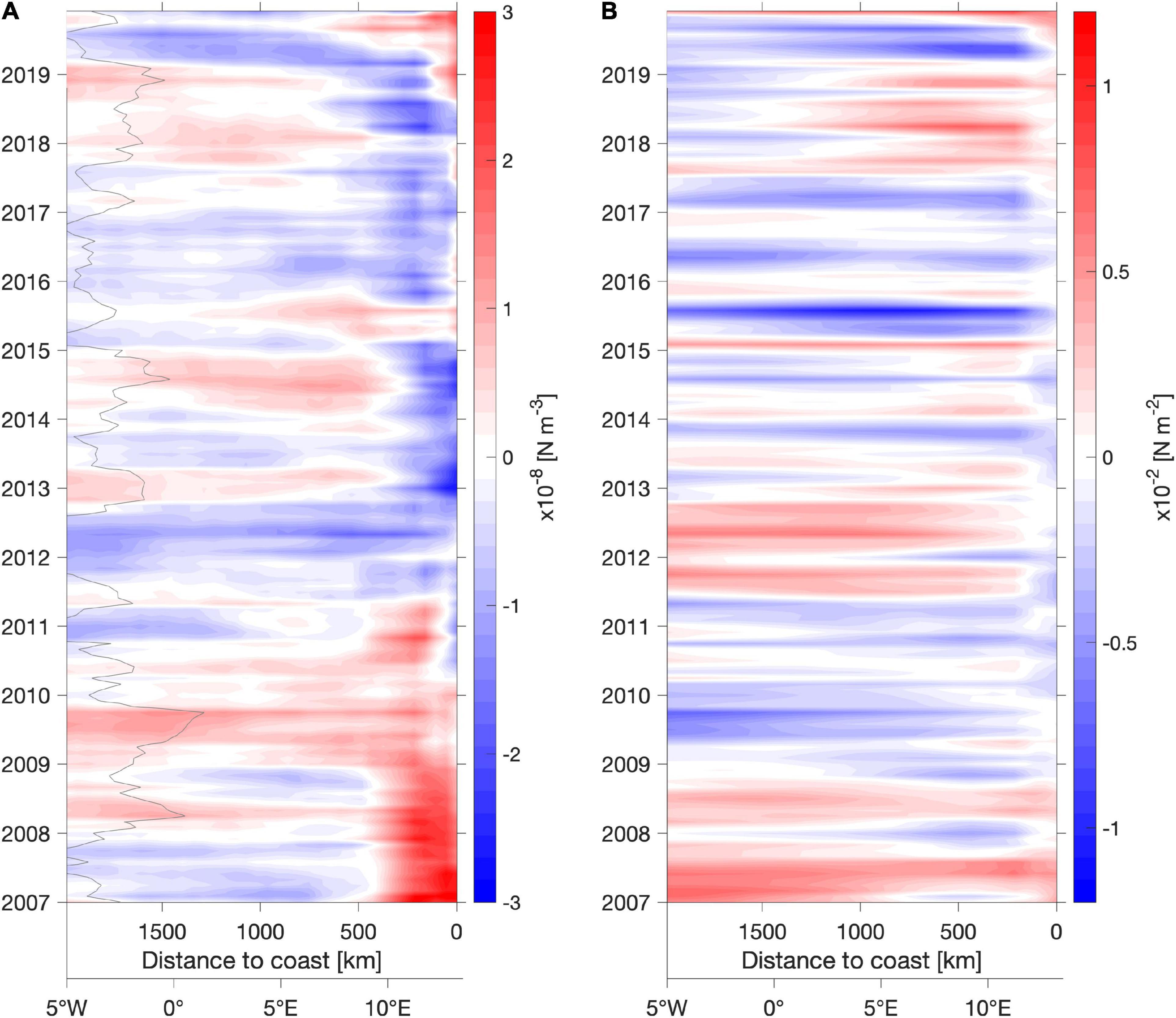
Figure 11. Six months running mean of (A) wind stress curl anomaly and (B) meridional wind stress anomaly meridionally averaged in SETA (10–20°S, 5°W–15°E) as a function of distance to the coast (at about 13.5°E) and time as inferred from Copernicus Marine environment monitoring service. Anomalies are computed relative to the monthly mean of the period of 2007–2019. Gray contour line in (A) indicates the zero-line of the mean wind stress curl, i.e., east of this line the mean wind stress curl is negative while west of this line it is positive.
Analysis of Latent Heat Fluxes, Evaporation and Specific Humidity
In order to investigate a possible forcing of the observed mixed layer changes, in this section decadal trends of latent heat flux, precipitation, specific humidity and evaporation are evaluated for the eastern tropical Atlantic. It is important to point out that the latent heat flux and specific humidity differ substantially among the two analyzed products.
The trend of OAFlux latent heat flux shows positive values in almost the entire eastern tropical Atlantic, i.e., the oceanic latent heat loss is reduced (Figure 12a). Only a region around 10°S, 10°W shows an increase in oceanic latent heat loss as well as an area south of 20°S close to the Namibian coast. Accordingly, decreasing evaporation trends are observed where latent heat loss is reduced (Figure 12c). Contrary, oceanic latent heat loss from TropFlux shows an increase south of 5°S away from the coast. North of 5°S including the Gulf of Guinea and along the coast the latent heat loss is decreasing (Figure 12d).
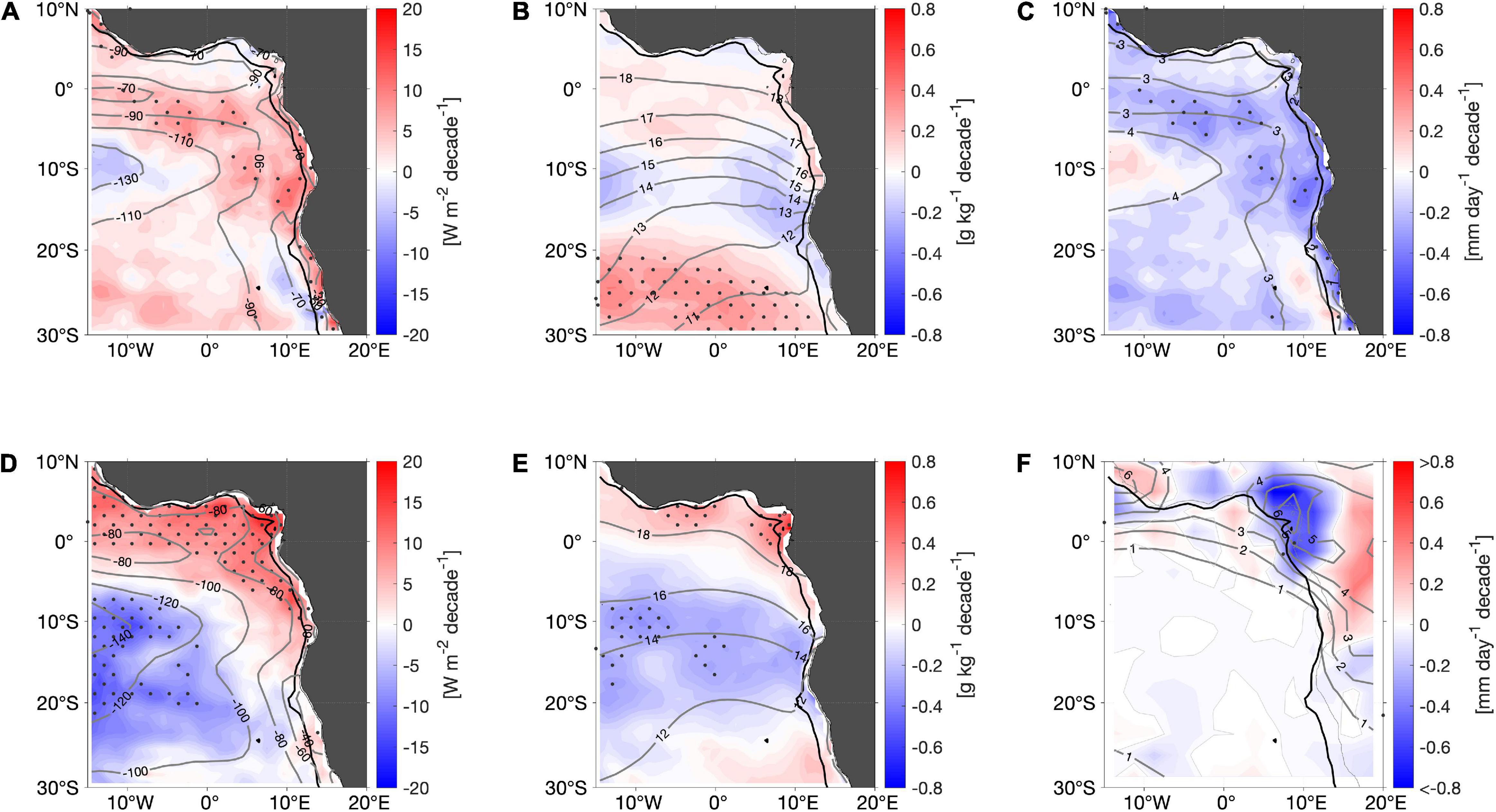
Figure 12. Decadal trend of (A) latent heat flux anomaly, (B) specific humidity anomaly, and (C) evaporation anomaly from OAFlux data (2006–2019) and (D) latent heat flux anomaly and (E) specific humidity anomaly from TropFlux data (2006–2018) as well as (F) precipitation anomaly of GPCP data (2006–2019). All anomalies are computed relative to the corresponding monthly means. Note, a negative latent heat flux indicates that the ocean loses heat. Gray contour lines show the corresponding mean field. Areas where the trend is of 95% significance are stippled. Black line indicates the 2,000 dbar isobath of the shelf region.
In addition, the trend of specific humidity of OAFlux reveals increasing humidity in the equatorial region while south of that region humidity is found to be reduced. Southward from 15°S humidity increases again (Figure 12b). For the TropFlux product humidity increases in the Gulf of Guinea and within the coastal regions extending southward to about 10°S (Figure 12e). The reduction of specific humidity is spatially larger than in OAFlux and even reaches up to 25–30°S. These differences among OAFlux and TropFlux highlight the uncertainties in the heat flux trends.
Besides, GPCP precipitation trend demonstrates a decline of precipitation in the area of the equatorial region, while slightly south of it the precipitation increases (Figure 12f). The Congo drainage basin reveals intensified precipitation rates.
Primary Production
The SETA upwelling system is a key region of enhanced nutrient supply to the euphotic zone that fuels local primary productivity. This section contrasts the observed signals in stratification with rates of net primary production derived from satellite observations.
The mean field of net primary production for the period of 2006–2019 shows elevated values especially within the eastern boundary regions and in the equatorial upwelling region (Figure 13A). The decadal trend pattern from the time series reveals that primary productivity in open ocean is increasing around 5–10% per decade almost everywhere in the eastern tropical Atlantic (Figure 13A). Specifically, in the SETA region primary production is intensifying as well (Figure 13A). North of the SETA region primary production depicts a small decreasing trend. The overall trend pattern correlates with the trend of the vertical stratification maximum except from the equatorial region, i.e., in general there is higher productivity in regions with enhanced stratification and shoaling stratification maximum (cf. Figures 4C,D, 13A).
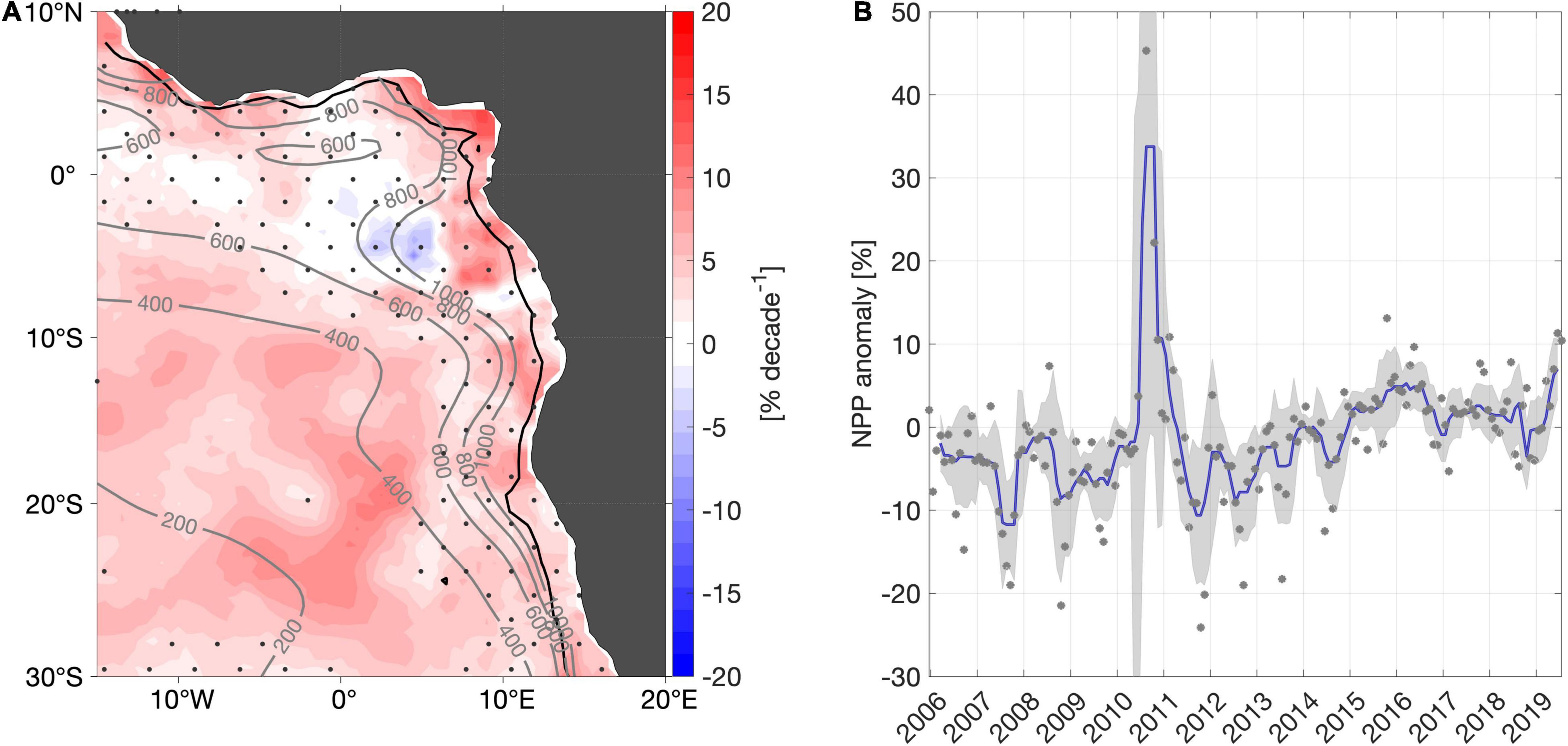
Figure 13. (A) Decadal trend of net primary production (NPP) deduced from satellite observations from Ocean Productivity site for the time period of 2006–2019. The decadal trend has been evaluated from the anomalies relative to the corresponding monthly means. Areas where the trend is not of 95% significance are stippled. The gray contour lines in (A) show the mean NPP field. The black contour line indicates the 2,000 dbar isobath of the shelf region. (B) Six months running median NPP anomaly in SETA region (10–20°S, 5°W–15°E) in percent (blue line). Anomalies are computed to the monthly mean. Shading denotes the standard deviation and dots refer to the given monthly values from the product.
Taking a closer look at the 6 months running median percental change of the net primary production in the SETA region, the time series of the median shows a maximum of above 30% primary production in 2010 (Figure 13B). Except from this maximum the primary productivity seems to increase in the SETA region. For the years 2012–2019 the productivity is continuously enhancing (Figure 13B).
Discussion
Physical Processes Leading to the Observed Stratification Changes
The findings of this study highlight locally large stratification increases within the upper 200 m in the tropical Atlantic Ocean for the Argo observation period of 2006–2019. Especially within the SETA region (10–20°S, 5°W–15°E) we observe an almost 60% intensification of the vertical stratification maximum from 2006 to 2020. This enhanced stratification is related to a warming, freshening and shoaling of the mixed layer. It represents a shift from subtropical stratification with salinity maximum water at the top toward a tropical stratification with warm and fresh surface waters (Figure 8). Mixed layer characteristics in the SETA region steadily change over time, i.e., changes are not confined to some single years. We observe a continuous warming of the mixed layer of 3°C during the years of 2006–2018 as well as a freshening of more than 0.5 g kg–1 from 2009 to 2020 (Figure 7). The MLT timeseries revealed a substantial temperature drop in 2019 which was followed by a warm mixed layer event at the end of the year (Figure 7). The negative MLT anomaly might be a result of an uneven distribution of the Argo profiles. The warm event in the beginning of 2020 can be associated to a Benguela Niño according to the classification given in Imbol Koungue et al. (2019).
Following the method of Bindoff and McDougall (1994) a pure warming or a pure freshening at a fixed depth for a typical subtropical stratification, as in the SETA region identified, should be the vector summation of negative spice and positive heave. Indeed, we observe the decline of spice on the isopycnals surrounding the vertical stratification maximum (Figure 7D). Yet, the isopycnals are rising (implying a negative heave, Figure 9A) and not deepening as anticipated for a pure warming or freshening process. Maximum upwelling of the isopycnals is observed about 10° offshore in the SETA region (Figure 6). Hence, another process has to be involved in the stratification increase. Wind stress curl-driven changes can lead to pure heaving (i.e., vertical adjustment of isopycnals) which is not associated with signatures in the T-S diagram (Bindoff and McDougall, 1994; Huang, 2015). In fact, we found an already negative wind stress curl becoming more negative in the SETA region, i.e., wind curl-driven upwelling is favored. As upwelling intensifies, isopycnals slope upward just as the time series show (Figure 9A). This suggests that the wind curl-driven upwelling is superimposed onto the pure warming and freshening processes discovered in the mixed layer and is obviously having a larger effect on the vertical displacement of the isopycnals. Besides, the heave mechanism does not contradict the stratification increase. The upper isopycnals are rising and thereby the distance between the 25.5 and the 26.0 kg m–3 is reducing and correspondingly the Brunt–Väisälä frequency is increasing (Figure 9). For the 26.5 kg m–3 isopycnal different processes seem to be involved. This deeper isopycnal is shoaling too, however, the distance between the 26.0 and the 26.5 kg m–3 isopycnals is becoming larger. Furthermore, the spice on the 26.5 kg m–3 isopycnal is slightly increasing (Figure 7). This indicates that stratification changes do not happen constantly at all depth levels which is confirmed by the T-S diagram with annual mean profiles of temperature and salinity (Figure 8) and by the mean Brunt–Väisälä frequency profiles for three different time periods (Figure 9B). At deeper levels (at the depth around the 26.5 kg m–3 isopycnal) the stratification is decreasing slightly (Figure 9).
Partly in contrast to the above noted findings related to the wind stress curl is that the meridional wind stress shows a shift from northward to southward anomalies within 200 km of the coast. This implies downwelling favorable conditions close to coast. However, southward wind stress anomalies could result in an increasing southward extent of near-equatorial surface waters approaching the SETA region and thereby altering the primarily subtropical stratification in the SETA region to more tropical conditions. In addition, we can compare the decadal trend pattern of wind speed and zonal wind stress, where the southern part of the SETA region reveals a slight intensification of the southeast trades. However, this area is surrounded by a westerly (positive) zonal wind stress trend, implying a weakening of the trades. Overall, it seems that the SASH is moving or extending poleward and thereby changing the prevailing winds near the African coast (Figure 11). Indeed, Zilli et al. (2019) found the SASH is extending further southwestward in the period of 2005–2014 compared to 1979–1991. Their results indicate that the shift produces a cyclonic anomaly of the wind over the tropical South Atlantic. Hence, this fits well to our observation of negative wind stress curl anomaly in the SETA region. Associated with the change of the SASH, the BLLCJ might have been modified, too. According to Patricola and Chang (2017), the BLLCJ shows a large intraseasonal variability linked to the SASH. Intense jet events are found to be aligned with a strengthened SASH and increased equatorward meridional wind stress 5–10° offshore from the coast in the SETA region. Further offshore and to the north of this region, however, they found that the meridional wind stress is reduced. This pattern is similar to what our results show on decadal timescales and thus, indicates that during the observational period of our study the BLLCJ might have strengthened and led to the associated wind stress changes. In addition, future projections of Lima et al. (2019b) also show that as a result of global warming the SASH is going to intensify and therefore amplify the pressure gradient toward the Angolan low pressure. This is further associated with a poleward movement of the SASH and is assumed to cause a wind speed increase around 26°S whereas north of 17.5°S the wind speed is going to be reduced.
Nonetheless, careful attention must be taken with satellite wind products as they often do not represent coastal areas very well. The statistical significance test shows how uncertain these products are which is a problem for climatic studies. Despite this uncertainty, it is still important to point out that the isopycnals are continuously shoaling which has to be a result of intensified wind curl-driven upwelling. It indicates that the observed wind stress data has to be trustworthy to some extent.
Changes of the latent heat flux, evaporation and specific humidity strongly depend on the used product (Figure 12). Following the decadal trends from OAFlux, the freshening of the mixed layer could be associated with a decreased oceanic latent heat loss and thus, reduced evaporation. Conversely, latent heat flux and humidity trends from TropFlux actually indicate a decline in humidity in most of the tropical South Atlantic and increased oceanic latent heat loss. Only close to the coast and in the equatorial region the heat loss is reduced. This would rather be a sign for a salinification of the mixed layer. The large uncertainty of the heat flux products makes it difficult to interpret our findings of the mixed layer changes. Also, the test of significance mirrors the great uncertainty of these products.
The GPCP precipitation data shows a rising trend in the drainage area of the Congo River. This might enhance river input and thus increase freshwater fluxes into the ocean. However, caution must be taken as precipitation data in the tropical regions is uncertain. In fact, different precipitation products show inconsistent variabilities in the tropical oceans (Sun et al., 2018 and references herein). The mean precipitation pattern is well-represented with GPCP data. Yet, there are large variations in regions with a small amount of gauge stations (Sun et al., 2018 and references herein). Besides, the significance analysis reveals barely anywhere significant trends. It is unfortunate that the meteorological data are so uncertain which makes it difficult to interpret and explain results from a climatic study like this one.
Despite the fact, that the Argo time series of the SETA region indicate mostly a steady increase or decline, we must be aware that there are uncertainties due to either an uneven distribution of the floats within the region as well as a minimum number of profiles in 2008. However, the time period of 2009–2018 shows an amount of 300 profiles and more per year allowing to achieve confident results.
As a matter of climate change, stratification is expected to increase due to the warming of ocean’s surface (Capotondi et al., 2012). Yamaguchi and Suga (2019) and most recently Li et al. (2020) highlighted the continuous enhancement of the stratification in the global oceans since the 1960s with largest impacts within the upper 200 m in the tropics. Comparing their global results to our findings of the last 13 years, does not yield guarantee that the increased stratification in the SETA region is a result of the on-going global warming. Probably, the much larger trends in the SETA region compared to the global trends suggest still internal climate variability as the main reason. However, also a poleward migration of the SASH that could be forced by climate warming would contribute to enhanced warming. Thus, also the superposition of different climate-warming induced processes could result in the observed regionally enhanced trends.
Comparison of Stratification and Mixed Layer Changes to Observations of Primary Productivity
Changes in the upper-ocean stratification matter as they affect not only physical ocean dynamics such as ocean ventilation processes but also biogeochemical and ecological activities such as nutrient fluxes and fisheries. Nevertheless, the consequences of increased stratification for upwelling regions are not yet fully understood (Jarre et al., 2015). The SETA upwelling system is a key region for enhanced nutrient supply to the euphotic zone and hence, a core nutrient source for high coastal primary productivity. The nutricline is just below the mixed layer depth and within the depth range of the vertical stratification maximum in this region. The location of the nutricline was checked from individual profiles (Schlitzer, 2021). The common assumption is that increased stratification as a result of global warming will weaken mixing processes that are responsible for the upward nutrient flux to the surface waters and thereby reducing the primary production (Capotondi et al., 2012). In contradiction, our findings reveal that the net primary productivity is actually rising since 2012 in the SETA region and thereby correlating with the increase in stratification but also warming, freshening and shoaling of the mixed layer as well as the depth of the stratification maximum. In fact, this fits to enhanced observed long-term trends of chlorophyll-a data off Angola and northern Benguela recently reported by Lamont et al. (2019). Additionally, Jarre et al. (2015) discussed increased chlorophyll-a in Northern Benguela from 2006 to 2010 which was found along with a warming of the sea surface and decreased coastal upwelling. They assume that the upwelling was still in favor for primary productivity and anomalous downwelling not strong enough to suppress mixing. Actually, our findings for the SETA region indicate increased wind curl-driven upwelling associated with shoaling depths of the stratification maximum and the mixed layer. This process could instead enhance the nutrient supply into the euphotic zone and could thus explain the rising rates of primary productivity in recent years.
Furthermore, given that except from the equatorial region the trends of primary production and stratification seem to coincide, this highlights the uncertainties and lack of understanding that we are still dealing with concerning the linkage between stratification and primary production. In fact, Lozier et al. (2011) identified that there exists a direct relationship between stratification and primary productivity on seasonal time scales. Nevertheless, they concluded that on longer time scales the two variables cannot be linked so easily anymore.
Our time series shows an outstanding event in 2010 of above 30% increase of primary productivity. According to Bachèlery et al. (2016), interannual variations in biogeochemistry (such as nitrate and oxygen) off Angola, Namibia and Benguela are mainly generated by remote equatorial forcing due to CTWs. These variations of nitrate and oxygen have a large influence on the chlorophyll and primary productivity. Indeed, Bachèlery et al. (2016) state that off Angola these events are responsible for up to 30% of the mean primary productivity. Hence, such an event could have contributed to this large maximum in primary productivity in 2010. An indicator for this could be the cold event in 2010 prior to the Benguela Niño in 2011 (Imbol Koungue et al., 2019). However, this is something we cannot prove with Argo observations as they are not able to represent CTWs.
Given that the net primary productivity data is based on a satellite product, the findings should be treated with caution. Satellite products of primary production are based on empirical models as from Behrenfeld and Falkowski (1997) and are no direct measurement. These models use satellite measurements of chlorophyll and SST. Satellites only measure the surface layer (Robinson, 2010). Hence, we do not know about the primary productivity at greater depth or if there is a vertical shift of biomass. There might be a compression of the primary productivity near the surface in case of thinner mixed layers, which would be better visible in satellite data. Nevertheless, compared to situations with thicker mixed layers, this could still imply a reduction of vertically integrated primary productivity.
Possible Implications for the Pelagic Fishes
Understanding the consequences of enhanced stratification on primary productivity is key as this will have further impact on the marine food web. In fact, small pelagic fishes are sensitive to climate variability (Bakun et al., 2015; López-Parages et al., 2020; Peck et al., 2021). For instance, variations in temperature and food availability can lead to migrations of small pelagic fishes and to changes of their behavior (Brochier et al., 2018; López-Parages et al., 2020). Our observed stratification transition from subtropical to tropical conditions associated with a warmer mixed layer is likely to impact the small pelagic fishes in the SETA region. We now propose a hypothesis on the physics-to-fish relation in this region, in particular concerning the coexistence of the sardinellas S. aurita preferring the warm tropical waters north of the ABF and the sardines S. sagax favoring cooler temperatures south of the ABF (BCC, 2012). The two stocks migrate seasonally following their temperature and habitat preferences, with the SETA region being the preferred habitat for adult sardinella during austral summer (Boley and Fréon, 1980). As a result of the warming mixed layer and increasing stratification, the ABF is shifting southward. This gives the tropical sardinellas the possibility to migrate southward to stay within their best spawning and feeding environment on an all-year basis. There are indications that the tropical sardinellas of all age classes may have colonized this region during the recent decade. Indeed, Ekau et al. (2018) observed a southward shift of sardinella larvae from southern Angola to northern Namibia in the past few years. Ostrowski and Barradas (2018) reported the increasing incidence of juvenile sardinellas in trawl catches from this region during recent years. Additionally, the Benguela Current Convention (BCC, 2012) reported an increasing biomass of sardinellas off Angola and at the same time, a reduction of sardine biomass off Angola associated with a southward shift of the ABF. Sardinellas and sardines are in no feeding competition but they favor different hydrographic conditions. Besides the hydrographic parameters, there are other factors, such as the bathymetry, that impact the distribution of sardinellas and sardines which cannot be neglected.
To conclude, our results regarding the warming mixed layer and thereby stratification increase, suggest an evolution from sardine to sardinella habitat in the SETA region. Therefore, fishermen will have to adapt to new circumstances which probably will lead to economic consequences. According to Bearak and Mooney (2019), six to seven species off Angola have almost disappeared in recent years from fishermens’ catches in the SETA waters, leading to substantial disturbances for the fishing industry of Southern Angola.
Conclusion
To summarize, this study gives an insight about recent stratification increase related to a change from subtropical toward tropical conditions in the SETA upwelling region. This is associated with mixed layer warming and freshening as well as intensified wind stress curl-driven upwelling. The impact on biological processes is still lacking of knowledge. Nevertheless, this study indicates, that the relationship between stratification and primary production is not that straight forward as previously thought. In contrast to climate projections, the satellite-derived primary production shows an increasing trend, which, however, remains to be verified by in situ data.
Data Availability Statement
Publicly available datasets were analyzed in this study. This data can be found here: Argo (2019). Argo float data and metadata from Global Data Assembly Centre (Argo GDAC) – Snapshot of Argo GDAC of November 13th 2019. SEANOE. https://doi.org/10.17882/42182#68322; Argo (2020). Argo float data and metadata from Global Data Assembly Centre (Argo GDAC) – Snapshot of Argo GDAC of November 25th 2020. SEANOE. https://doi.org/10.17882/42182#78698; Brandt, Peter, Hahn, Johannes, Schmidtko, Sunke, Tuchen, Franz Philip, Kopte, Robert, Kiko, Rainer, Bourlès, Bernard, Czeschel, Rena, and Dengler, Marcus. (2021). Data and scripts used in “Atlantic Equatorial Undercurrent intensification counteracting warming induced deoxygenation” (Version 2) [Data set]. Zenodo. https://doi.org/10.5281/zenodo.4478285; Climate Data Guide: GPCP (Monthly): Global Precipitation Climatology Project. https://climatedataguide.ucar.edu/climate-data/gpcp-monthly-global-precipitation-climatology-project; Ocean Productivity Site: http://orca.science.oregonstate.edu/1080.by.2160.monthly.hdf.eppley.m.chl.m.sst.php; TropFlux – Indian National Centre for Ocean Information Services: latent heat and specific humidity: https://incois.gov.in/tropflux/tf_products.jsp; WHOI OAFlux: latent heat, evaporation and specific humidity: https://oaflux.whoi.edu/data-access/; Wind TAC (2018): WIND_GLO_PHY_CLIMATE_L4_REP_012_003 – Global Ocean Wind L4 Reprocessed Monthly Mean Observations, E.U. Copernicus Marine Service Information. Available at: https://resources.marine.copernicus.eu/?option=com_csw&view= details&product_id=WIND_GLO_PHY_CLIMATE_L4_REP_ 012_003.
Author Contributions
MR, PB, and SS designed the study and analyzed the data. MR and SS developed the method to obtain the Brunt–Väisälä frequency by using the Argo observation array. FVV and MO provided their expertise on small pelagic fishes and their habitat. MR drafted the manuscript. All authors contributed to the writing of the manuscript.
Funding
This study was supported by the EU H2020 TRIATLAS project under grant agreement 817578 and by the German Federal Ministry of Education and Research as part of the BANINO project (03F0795A).
Conflict of Interest
The authors declare that the research was conducted in the absence of any commercial or financial relationships that could be construed as a potential conflict of interest.
Publisher’s Note
All claims expressed in this article are solely those of the authors and do not necessarily represent those of their affiliated organizations, or those of the publisher, the editors and the reviewers. Any product that may be evaluated in this article, or claim that may be made by its manufacturer, is not guaranteed or endorsed by the publisher.
Acknowledgments
We acknowledge the WHOI OAFlux project (http://oaflux.whoi.edu) funded by NOAA Climate Observations and Monitoring (COM) program for providing the global ocean heat flux and evaporation products and TropFlux data which is produced under a collaboration between Laboratoire d’Océanographie et du climat : Expérimentations et Approches Numériques (LOCEAN) from Institut Pierre Simon Laplace (IPSL, Paris, France) and National Institute of Oceanography/CSIR (NIO, Goa, India), and supported by Institut de Recherche pour le Développement (IRD, France) for the heat flux product. TropFlux relies on data provided by the ECMWF Re-Analysis interim (ERA-I) and ISCCP projects. Additionally, we acknowledge the Climate Data Guide: GPCP (Monthly): Global Precipitation Climatology Project. Achieved from https://climatedataguide.ucar.edu/climate-data/gpcp-monthly-global-precipitation-climatology-project. Furthermore, this study has been conducted using E. U. Copernicus Marine Service Information for the wind stress product.
Supplementary Material
The Supplementary Material for this article can be found online at: https://www.frontiersin.org/articles/10.3389/fmars.2021.748383/full#supplementary-material
Footnotes
- ^ https://oaflux.whoi.edu/data-access/
- ^ http://sites.science.oregonstate.edu/ocean.productivity/index.php
References
Adler, R. F., Sapiano, M. R., Huffman, G. J., Wang, J. J., Gu, G., Bolvin, D., et al. (2018). The global precipitation climatology project (GPCP) monthly analysis (New Version 2.3) and a review of 2017 global precipitation. Atmosphere 9:138. doi: 10.3390/atmos9040138
Akima, H. (1970). A new method of interpolation and smooth curve fitting based on local procedures. J. ACM 17, 589–602. doi: 10.1145/321607.321609
Argo (2019). Argo Float Data and Metadata From Global Data Assembly Centre (Argo GDAC) – Snapshot of Argo GDAC of November 13st 2019. SEANOE. doi: 10.17882/42182#68322
Argo (2020). Argo Float Data and Metadata From Global Data Assembly Centre (Argo GDAC) – Snapshot of Argo GDAC of November 25st 2020. SEANOE. doi: 10.17882/42182#78698
Bachèlery, M. L., Illig, S., and Dadou, I. (2016). Forcings of nutrient, oxygen, and primary production interannual variability in the southeast Atlantic Ocean. Geophys. Res. Lett. 43, 8617–8625. doi: 10.1002/2016gl070288
Bakun, A., Black, B. A., Bograd, S. J., Garcia-Reyes, M., Miller, A. J., Rykaczewski, R. R., et al. (2015). Anticipated effects of climate change on coastal upwelling ecosystems. Curr. Clim. Change Rep. 1, 85–93. doi: 10.1007/s40641-015-0008-4
BCC (2012). Benguela Current Commission: State of Stocks Report. Report No. 2. Available online at: http://www.benguelacc.org/index.php/en/component/docman/doc_download/120-sos-report-2012-low (accessed April 19, 2021).
Bearak, M., and Mooney, C. (2019). 2°C Beyond the Limit. A Crisis in the Water is Decimating this Once-Booming Fishing Town. Washington Post. Available online at: https://www.washingtonpost.com/graphics/2019/world/climate-environment/angola-climate-change/ (accessed January 13, 2021).
Behrenfeld, M. J., and Falkowski, P. G. (1997). Photosynthetic rates derived from satellite-based chlorophyll concentration. Limnol. Oceanogr. 42, 1–20.
Bentamy, A. (2020). Product User Manual for Wind Product - WIND_GLO_PHY_CLIMATE_L4_REP_012_003, 1, 2 Edn. E.U. Copernicus Marine Service Information. Available online at: https://resources.marine.copernicus.eu/documents/PUM/CMEMS-WIND-PUM-012-003.pdf (accessed May 5, 2021).
Bentamy, A., and Fillon, D. C. (2012). Gridded surface wind fields from Metop/ASCAT measurements. Int. J. Remote Sens. 33, 1729–1754. doi: 10.1080/01431161.2011.600348
Bindoff, N. L., and McDougall, T. J. (1994). Diagnosing climate change and ocean ventilation using hydrographic data. J. Phys. Oceanogr. 24, 1137–1152. doi: 10.1175/1520-0485(1994)024<1137:dccaov>2.0.co;2
Boley, T., and Fréon, P. (1980). “Coastal pelagic resources,” in The Fish Resources of the Eastern Central Atlantic. Part One: The Resources of the Gulf of Guinea from Angola to Mauritania. FAO Fisheries Technical Paper No. 186.1, eds J. P. Troadec and S. Garcia (Rome: FAO), 13–76.
Brandt, P., Hahn, J., Schmidtko, S., Tuchen, F. P., Kopte, R., Kiko, R., et al. (2021). Atlantic Equatorial Undercurrent intensification counteracting warming induced deoxygenation. Nat. Geosci. 14, 278–282. doi: 10.1038/s41561-021-00716-1
Brochier, T., Auger, P. A., Pecquerie, L., Machu, E., Capet, X., Thiaw, M., et al. (2018). Complex small pelagic fish population patterns arising from individual behavioral responses to their environment. Prog. Oceanogr. 164, 12–27. doi: 10.1016/j.pocean.2018.03.011
Capotondi, A., Alexander, M. A., Bond, N. A., Curchitser, E. N., and Scott, J. D. (2012). Enhanced upper ocean stratification with climate change in the CMIP3 models. J. Geophys. Res. Oceans 117, 1–23. doi: 10.1029/2011JC007409
Clément, L., McDonagh, E. L., Marzocchi, A., and Nurser, A. J. (2020). Signature of ocean warming at the mixed layer base. Geophys. Res. Lett. 47, 1–10. doi: 10.1029/2019GL086269
Desbruyères, D., McDonagh, E. L., King, B. A., and Thierry, V. (2017). Global and full-depth ocean temperature trends during the early twenty-first century from Argo and repeat hydrography. J. Clim. 30, 1985–1997. doi: 10.1175/JCLI-D-16-0396.1
Ekau, W., Auel, H., Hagen, W., Koppelmann, R., Wasmund, N., Bohata, K., et al. (2018). Pelagic key species and mechanisms driving energy flows in the northern Benguela upwelling ecosystem and their feedback into biogeochemical cycles. J. Mar. Syst. 188, 49–62. doi: 10.1016/j.jmarsys.2018.03.001
Fennel, W., Junker, T., Schmidt, M., and Mohrholz, V. (2012). Response of the Benguela upwelling systems to spatial variations in the wind stress. Cont. Shelf Res. 45, 65–77. doi: 10.1016/j.csr.2012.06.004
Fennel, W., and Lass, H. U. (2007). On the impact of wind curls on coastal currents. J. Mar. Syst. 68, 128–142. doi: 10.1016/j.jmarsys.2006.11.004
Feucher, C. (2016). Stratification Structure in Subtropical Gyres and its Decadal Variability in the North Atlantic Ocean. Doctoral dissertation. Brest: Université de Bretagne Occidentale.
Florenchie, P., Reason, C. J. C., Lutjeharms, J. R. E., Rouault, M., Roy, C., and Masson, S. (2004). Evolution of interannual warm and cold events in the southeast Atlantic Ocean. J. Clim. 17, 2318–2334. doi: 10.1175/1520-0442(2004)017<2318:eoiwac>2.0.co;2
Gammelsrød, T., Bartholomae, C. H., Boyer, D. C., Filipe, V. L. L., and O’toole, M. J. (1998). Intrusion of warm surface water along the Angolan Namibian coast in February–March 1995: the 1995 Benguela Niño. Afr. J. Mar. Sci. 19, 41–56.
Häkkinen, S., Rhines, P. B., and Worthen, D. L. (2016). Warming of the global ocean: spatial structure and water-mass trends. J. Clim. 29, 4949–4963. doi: 10.1175/JCLI-D-15-0607.1
Holte, J., and Talley, L. (2009). A new algorithm for finding mixed layer depths with applications to Argo data and Subantarctic Mode Water formation. J. Atmos. Ocean. Technol. 26, 1920–1939. doi: 10.1175/2009JTECHO543.1
Huang, R. X. (2015). Heaving modes in the world oceans. Clim. Dyn. 45, 3563–3591. doi: 10.1007/s00382-015-2557-6
Imbol Koungue, R. A., and Brandt, P. (2021). Impact of intraseasonal waves on Angolan warm and cold events. J. Geophys. Res. Oceans 126:e2020JC017088. doi: 10.1029/2020JC017088
Imbol Koungue, R. A., Rouault, M., Illig, S., Brandt, P., and Jouanno, J. (2019). Benguela Niños and Benguela Niñas in forced ocean simulation from 1958 to 2015. J. Geophys. Res. Oceans 124, 5923–5951. doi: 10.1029/2019JC015013
Ito, T., Long, M. C., Deutsch, C., Minobe, S., and Sun, D. (2019). Mechanisms of low-frequency oxygen variability in the North Pacific. Glob. Biogeochem. Cycles 33, 110–124. doi: 10.1029/2018GB005987
Jarre, A., Hutchings, L., Kirkman, S. P., Kreiner, A., Tchipalanga, P. C. M., Kainge, P., et al. (2015). Synthesis: climate effects on biodiversity, abundance and distribution of marine organisms in the Benguela. Fish. Oceanogr. 24, 122–149. doi: 10.1111/fog.12086
Keeling, R. F., Körtzinger, A., and Gruber, N. (2010). Ocean deoxygenation in a warming world. Annu. Rev. Mar. Sci. 2, 199–229. doi: 10.1146/annurev.marine.010908.163855
Kopte, R., Brandt, P., Claus, M., Greatbatch, R. J., and Dengler, M. (2018). Role of equatorial basin-mode resonance for the seasonal variability of the Angola current at 11°S. J. Phys. Oceanogr. 48, 261–281. doi: 10.1175/jpo-d-17-0111.1
Kopte, R., Brandt, P., Dengler, M., Tchipalanga, P. C. M., Macuéria, M., and Ostrowski, M. (2017). The Angola current: flow and hydrographic characteristics as observed at 11°S. J. Geophys. Res. Oceans 122, 1177–1189. doi: 10.1002/2016jc012374
Lamont, T., Barlow, R. G., and Brewin, R. J. W. (2019). Long-term trends in phytoplankton chlorophyll a and size structure in the Benguela upwelling system. J. Geophys. Res. Oceans 124, 1170–1195. doi: 10.1029/2018JC014334
Li, G., Cheng, L., Zhu, J., Trenberth, K. E., Mann, M. E., and Abraham, J. P. (2020). Increasing ocean stratification over the past half-century. Nat. Clim. Change 10, 1116–1123. doi: 10.1038/s41558-020-00918-2
Lima, D. C., Soares, P. M., Semedo, A., Cardoso, R. M., Cabos, W., and Sein, D. V. (2019a). A climatological analysis of the Benguela coastal low-level jet. J. Geophys. Res. Atmos. 124, 3960–3978. doi: 10.1029/2018jd028944
Lima, D. C., Soares, P. M., Semedo, A., Cardoso, R. M., Cabos, W., and Sein, D. V. (2019b). How will a warming climate affect the Benguela coastal low-level wind jet? J. Geophys. Res. Atmos. 124, 5010–5028. doi: 10.1029/2018jd029574
López-Parages, J., Auger, P. A., Rodríguez-Fonseca, B., Keenlyside, N., Gaetan, C., Rubino, A., et al. (2020). El Niño as a predictor of round Sardinella distribution along the northwest African coast. Prog. Oceanogr. 186:102341. doi: 10.1016/j.pocean.2020.102341
Lozier, M. S., Dave, A. C., Palter, J. B., Gerber, L. M., and Barber, R. T. (2011). On the relationship between stratification and primary productivity in the North Atlantic. Geophys. Res. Lett. 38:L18609. doi: 10.1029/2011GL049414
Lübbecke, J. F., Böning, C. W., Keenlyside, N. S., and Xie, S. P. (2010). On the connection between Benguela and equatorial Atlantic Niños and the role of the South Atlantic Anticyclone. J. Geophys. Res. Oceans 115:C09015. doi: 10.1029/2009JC005964
Lübbecke, J. F., Brandt, P., Dengler, M., Kopte, R., Lüdke, J., Richter, I., et al. (2019). Causes and evolution of the southeastern tropical Atlantic warm event in early 2016. Clim. Dyn. 53, 261–274. doi: 10.1007/s00382-018-4582-8
MathWorks, Inc (2019). Help Center: Makima. Natick, MA. Available online at: https://de.mathworks.com/help/matlab/ref/makima.html (accessed June 25, 2021).
McDougall, T. J., and Barker, P. M. (2011). Getting Started with TEOS-10 and the Gibbs Seawater (GSW) Oceanographic Toolbox, SCOR/IAPSO WG127. 28. Available online at: www.TEOS-10.org
Ostrowski, M., and Barradas, A. (2018). Report on the Evolution of the Angolan sardinella Stock in Relation to the Seasonal Coastally Trapped Waves Climatology and Interannual Equatorial Events 1994-2014, Extended Abstract, 2 pp., in PREFACE Deliverable D12.4, “Climate Variability and Pelagic Fish”, 26. Available online at: https://preface.w.uib.no/files/2018/11/PREFACE-D12.4-final-20180501.pdf (accessed June 30, 2021).
Ostrowski, M., Da Silva, J. C., and Bazik-Sangolay, B. (2009). The response of sound scatterers to El Niño-and La Niña-like oceanographic regimes in the southeastern Atlantic. ICES J. Mar. Sci. 66, 1063–1072. doi: 10.1093/icesjms/fsp102
Patricola, C. M., and Chang, P. (2017). Structure and dynamics of the Benguela low-level coastal jet. Clim. Dyn. 49, 2765–2788. doi: 10.1007/s00382-016-3479-7
Peck, M. A., Alheit, J., Bertrand, A., Catalán, I. A., Garrido, S., Moyano, M., et al. (2021). Small pelagic fish in the new millennium: a bottom-up view of global research effort. Prog. Oceanogr. 191:102494. doi: 10.1016/j.pocean.2020.102494
Pendergrass, A., Wang, J.-J., and National Center for Atmospheric Research Staff (2020). The Climate Data Guide: GPCP (Monthly): Global Precipitation Climatology Project. Available online at: https://climatedataguide.ucar.edu/climate-data/gpcp-monthly-global-precipitation-climatology-project (accessed November 06, 2020).
Peterson, R. G., and Stramma, L. (1991). Upper-level circulation in the South Atlantic Ocean. Prog. Oceanogr. 26, 1–73. doi: 10.1016/0079-6611(91)90006-8
Potts, W. M., Henriques, R., Santos, C. V., Munnik, K., Ansorge, I., Dufois, F., et al. (2014). Ocean warming, a rapid distributional shift, and the hybridization of a coastal fish species. Glob. Change Biol. 20, 2765–2777. doi: 10.1111/gcb.12612
Praveen Kumar, B., Vialard, J., Lengaigne, M., Murty, V. S. N., and McPhaden, M. J. (2012). TropFlux: air-sea fluxes for the global tropical oceans—description and evaluation. Clim. Dyn. 38, 1521–1543. doi: 10.1007/s00382-011-1115-0
Rhein, M., Rintoul, S. R., Aoki, S., Campos, E., Chambers, D., Feely, R. A., et al. (2013). “Observations: ocean,” in Climate Change 2013: The Physical Science Basis. Contribution of Working Group I to the Fifth Assessment Report of the Intergovernmental Panel on Climate Change, eds T. F. Stocker, D. Qin, G.-K. Plattner, M. Tignor, S. K. Allen, J. Boschung, et al. (Cambridge: Cambridge University Press).
Risien, C. M., Reason, C. J. C., Shillington, F. A., and Chelton, D. B. (2004). Variability in satellite winds over the Benguela upwelling system during 1999–2000. J. Geophys. Res. Oceans 109:C03010. doi: 10.1029/2003JC001880
Robinson, I. S. (2010) “Ocean biology from space,” in Discovering the Ocean from Space. Springer Praxis Books, 1st Edn. ed. P. Blondel (Berlin: Springer), 255–267. doi: 10.1007/978-3-540-68322-3_7
Roemmich, D., Church, J., Gilson, J., Monselesan, D., Sutton, P., and Wijffels, S. (2015). Unabated planetary warming and its ocean structure since 2006. Nat. Clim. Change 5, 240–245. doi: 10.1038/nclimate2513
Rouault, M. (2012). Bi-annual intrusion of tropical water in the northern Benguela upwelling. Geophys. Res. Lett. 39:L12606. doi: 10.1029/2012GL052099
Rouault, M., Illig, S., Bartholomae, C., Reason, C. J. C., and Bentamy, A. (2007). Propagation and origin of warm anomalies in the Angola Benguela upwelling system in 2001. J. Mar. Syst. 68, 473–488. doi: 10.1016/j.jmarsys.2006.11.010
Rouault, M., Illig, S., Lübbecke, J., and Koungue, R. A. I. (2018). Origin, development and demise of the 2010–2011 Benguela Niño. J. Mar. Syst. 188, 39–48. doi: 10.1016/j.jmarsys.2017.07.007
Sallée, J.-B., Pellichero, V., Akhoudas, C., Pauthenet, E., Vignes, L., Schmidtko, S., et al. (2021). Summertime increases in upper-ocean stratification and mixed-layer depth. Nature 591, 592–598. doi: 10.1038/s41586-021-03303-x
Schlitzer, R. (2021). Ocean Data View. Available online at: odv.awi.de (acceseed September 06, 2021).
Shannon, L. V., Agenbag, J. J., and Buys, M. E. L. (1987). Large-and mesoscale features of the Angola-Benguela front. S. Afr. J. Mar. Sci. 5, 11–34. doi: 10.2989/025776187784522261
Shannon, L. V., Boyd, A. J., Brundrit, G. B., and Taunton-Clark, J. (1986). On the existence of an El Niño-type phenomenon in the Benguela system. J. Mar. Res. 44, 495–520.
Siegfried, L., Schmidt, M., Mohrholz, V., Pogrzeba, H., Nardini, P., Böttinger, M., et al. (2019). The tropical-subtropical coupling in the Southeast Atlantic from the perspective of the northern Benguela upwelling system. PLoS One 14:e0210083. doi: 10.1371/journal.pone.0210083
Somavilla, R., González-Pola, C., and Fernández-Diaz, J. (2017). The warmer the ocean surface, the shallower the mixed layer. how much of this is true? J. Geophys. Res. Oceans 122, 7698–7716. doi: 10.1002/2017JC013125
Sun, Q., Miao, C., Duan, Q., Ashouri, H., Sorooshian, S., and Hsu, K. L. (2018). A review of global precipitation data sets: data sources, estimation, and intercomparisons. Rev. Geophys. 56, 79–107. doi: 10.1002/2017RG000574
Tchipalanga, P., Dengler, M., Brandt, P., Kopte, R., Macuéria, M., Coelho, P., et al. (2018). Eastern boundary circulation and hydrography off Angola: building Angolan oceanographic capacities. Bull. Am. Meteorol. Soc. 99, 1589–1605. doi: 10.1175/bams-d-17-0197.1
Wind TAC (2018). WIND_GLO_PHY_CLIMATE_L4_REP_012_003 - Global Ocean Wind L4 Reprocessed Monthly Mean Observations. E.U. Copernicus Marine Service Information. Available online at: https://resources.marine.copernicus.eu/?option=com_csw&view=details&product_id=WIND_GLO_PHY_CLIMATE_L4_REP_012_003 (accessed August 14, 2020).
Yamaguchi, R., and Suga, T. (2019). Trend and variability in global upper-ocean stratification since the 1960s. J. Geophys. Res. Oceans 124, 8933–8948. doi: 10.1029/2019JC015439
Yu, L., Jin, X., and Weller, R. A. (2008). Multidecade Global Flux Datasets from the Objectively Analyzed Air-Sea Fluxes (OAFlux) Project: Latent and Sensible Heat Fluxes, Ocean Evaporation, and Related Sur- Face Meteorological Variables. OAFlux Project Technical Report. OA-2008-01. Woods Hole, MA: Woods Hole Oceanographic Institution.
Zeng, Z., Brandt, P., Lamb, K. G., Greatbatch, R. J., Dengler, M., Claus, M., et al. (2021). Three-dimensional numerical simulations of internal tides in the Angolan upwelling region. J. Geophys. Res. Oceans 126:e2020JC016460. doi: 10.1029/2020JC016460
Keywords: southeastern tropical Atlantic Ocean, decadal variability, upper-ocean stratification increase, mixed layer warming and freshening, heave and spice anomalies, primary productivity
Citation: Roch M, Brandt P, Schmidtko S, Vaz Velho F and Ostrowski M (2021) Southeastern Tropical Atlantic Changing From Subtropical to Tropical Conditions. Front. Mar. Sci. 8:748383. doi: 10.3389/fmars.2021.748383
Received: 27 July 2021; Accepted: 29 October 2021;
Published: 26 November 2021.
Edited by:
Fabrice Hernandez, Institut de Recherche Pour le Développement (IRD), FranceReviewed by:
Zhongxiang Zhao, University of Washington, United StatesRu Chen, Tianjin University, China
Copyright © 2021 Roch, Brandt, Schmidtko, Vaz Velho and Ostrowski. This is an open-access article distributed under the terms of the Creative Commons Attribution License (CC BY). The use, distribution or reproduction in other forums is permitted, provided the original author(s) and the copyright owner(s) are credited and that the original publication in this journal is cited, in accordance with accepted academic practice. No use, distribution or reproduction is permitted which does not comply with these terms.
*Correspondence: Marisa Roch, mroch@geomar.de