Introduction to Adsorption: Kinetics and Thermodynamics

Adsorption serves as the foundation for numerous water treatment technologies and plays a crucial role in understanding the interactions among materials and the molecules/ions in solution. Consequently, I have prepared this article summarizing some of the fundamental concepts of this subject using a batch adsorbate/adsorbent reaction model perspective.

Introduction to adsorption

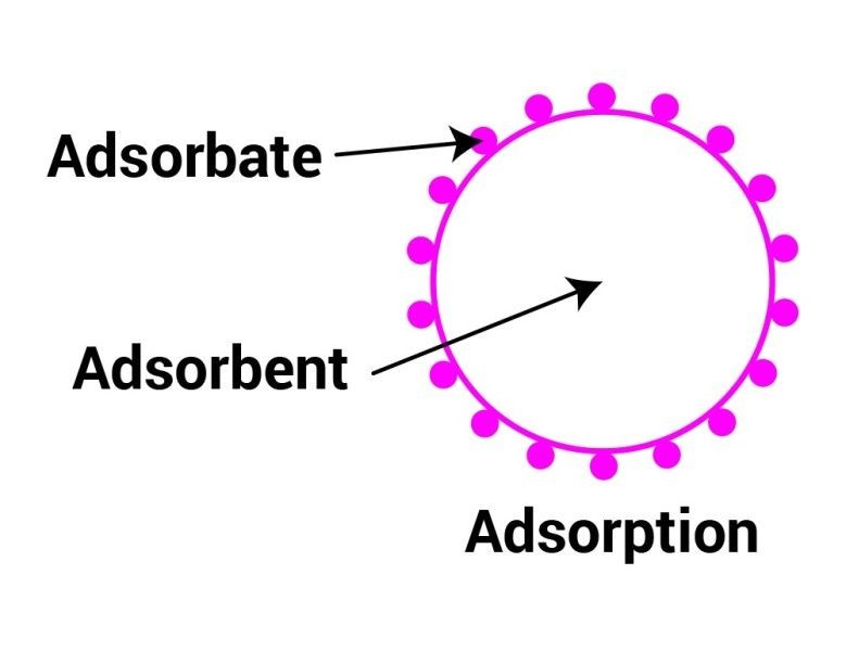
Adsorption is a process where ions and/or molecules interact physically or bind chemically to the surface of an adsorbent. Physisorption primarily involves weak van der Waals interactions, whereas chemisorption involves attachment to the surface through a process that entails the formation of bonds.

The adsorption of an adsorbate A in solution onto a adsorbent M can be described by the following equation:

A(aq)+M(s) ⇋ AM(s) (eq. 1)

Even though eq. 1 seems simple, the adsorption process may involve several steps before adsorbate A settles on the surface. It is important to note that the adsorbate will move through the solution via diffusion and advection/convection. If the adsorbate is charged, migration (electromigration) has to be considered. These three mass transfer mechanisms are supported by the Nernst-Planck equation shown in eq. 2 and 3:

Where J is the flux of particles -or adsorbate in this case-,

Furthermore, the mechanism by which adsorbate A approaches and further interacts or reacts with the surface of the adsorbent can be summarized in the following steps shown in Figure 1.

1. The adsorbate A diffuses, migrates (if charged) or convects/advects from the bulk of the solution to the static film, also called boundary layer, surrounding the adsorbent particle.

2. The adsorbate A diffuses, migrates (if charged) through the static film until it reaches the surface. 

3. If the adsorbent is porous the adsorbate A will enter through the pores via intraparticle diffusion. Migration may play a role if it the adsorbate is charged (e.g. ion).

4. The adsorbate A settles on an available site by a physical or a chemical interaction. 

If the process is under high Reynolds the diffusion from the bulk of the solution of A (step 1) to the boundary layer can be neglected. Also the thickness of the static liquid film surrounding the adsorbent particle can be diminished by increasing the Reynolds number making it possible to significantly reduce the effect of diffusion through the static liquid film (step 2).

1. Adsorption Kinetics

As early as the year 1898, kinetics of the adsorption were studied for the adsorption of oxalic-manolic acid onto charcoal by Lagergren [1]. Several kinetic models have been developed since then, including the Elovich equation derived from the work of Zeldowitsch in 1934 on the sorption of carbon monoxide onto manganese dioxide [2]. In order to distinguish these models from standard chemical kinetics the literature refers to them as pseudo-order models [2], despite the fact that this term is widely used in physical chemistry for orders different from an integer ≥ 0. 

Adsorbate concentration on the surface of the solid is expected to increase with decreasing rate over time as sites on the adsorbent become occupied. Hence the rate of the reaction will follow the form:

Where k is the rate constant, xeq is the concentration of the adsorbate on the surface of the adsorbent as t 🡪 ∞ and n is the exponent that in the case of fitting to kinetic curves will be the order of the reaction, normally related to the reaction mechanism (e.g. unimolecular, bimolecular, etc…). As in standard chemical kinetics the order of the model reflects the way that the concentration changes over time. For example, in a first-order kinetic expression the exponential in the rate expression is 1 in respect to the concentrations of the reagents. In pseudo-first-order models the exponential is also 1 but in respect to the available sites remaining. Often the kinetic relation is plotted as the amount of adsorbate per mass of adsorbent (e.g.  mmol g-1) as a function of time. If the experimental data is modelled using these equations the rate constant may be obtained.

Prof. Yuh-Shan Ho [2] states that pseudo-first order kinetic models are more likely to fit adsorption processes describing the uptake of adsorbate from solution onto a solid adsorbent in which the rate-limiting step is diffusion (eg. intraparticle, film diffusion), while pseudo-second order kinetics models are more likely to fit processes in which the rate-limiting step is the chemisorption of the involved species. 

1. Pseudo-first order

Pseudo-first order equations have been widely used for obtaining kinetic parameters in the literature [2,3]. The Lagergren equation is the first known mathematical description of sorption kinetics. The rate equation is given by,

where t is the time in min, qe and qt are in mmol g-1 and represent the sorption capacities at the equilibrium and time t, k is the rate constant in min-1. The rate of sorption is proportional to a constant and the amount of available sites left.

Integrating eq. 5 between the boundary conditions t = 0 to t = t and qt = 0 to qt = qt yields, 

or in the linear form,

By plotting log (qe – qt) as a function of t, the kinetic rate constant and the sorption capacity at the equilibrium for the given experimental conditions may be obtained from the slope and intercept, respectively.

1. Pseudo-second order

A pseudo-second order model was first introduced by Blanchard in 1984 [4] which described the sorption of divalent metal ions onto a zeolite by an ion exchange mechanism. Where the zeolite exchanged 2 moles of ammonium ions for 1 mole of divalent metals as shown in eq. 8.

Blanchard represented this process as a differential equation that depicts the rate of sorption as being proportional to a rate constant and to the square of the remaining unoccupied sites:

where, t is the time in min, qt is the amount adsorbed at the time t in mmol g-1, k is the kinetic constant in g mmol-1 min-1 and qe is a constant that represents the amount adsorbed at the equilibrium in mmol g-1 (when t 🡪 ∞) . In 1999 McKay and Ho [5] presented a pseudo-second order model based on Blanchard’s differential equation and gave further meaning to the constants. By integrating between the boundaries t = 0 to t = t and qt = 0 and qt = qt and re-arranging, eq. 10 is obtained.

Rearranging eq. 10 to a linear form, eq. 11 is obtained,

Plotting t/qt against t, allows qe and k to be obtained from the slope and intercept respectively. In this model kqe2 is often written as h and is the initial sorption speed in mmol g-1 min-1. This model has been successfully used to model the sorption of compounds in aqueous solutions onto solid adsorbents in various publications [3-8].

1. Activation energy

The kinetic rate constants obtained by the pseudo order models shown in this section can be used to obtain the activation energy (Ea) of the process through an Arrehnius plot represented by eq. 12 [7]. 

where k is the kinetic rate constant obtained by any of the kinetic models, discussed in Section 4, Ea is the activation energy in J mol-1, A is a correlation factor, R is the gas constant 8.314 J mol-1 K-1 and T is the temperature in K. By plotting ln k as a function of T-1 the value of Ea can be obtained from the slope. Ea is important since it suggests if the nature of the sorption is either physical or chemical. The activation energy for physical adsorption mechanisms are reported to be in the range of 5 to 30 kJ mol-1, while chemical adsorption mechanisms are commonly between 40 – 800 kJ mol-1 [8]. The value obtained by this mathematical analysis gives a suggestion for what the nature of the process could be, since in the adsorption process many steps are involved and the value may change with the adsorbent and adsorbate being used. 

Thermodynamics of Adsorption: Studying the equilibrium of the adsorption process

Adsorption Isotherms

If both adsorbate and sorbent are left for a sufficient time the adsorption process will reach equilibrium. This happens when both forward (adsorption) and backward (desorption) processes reach the same rate. In the literature several mathematical equations have been reported that help to model the equilibrium of the sorption, but many fail to give useful information as they do not possess strong thermodynamic explanation. In this article the Langmuir, Freundlich and Temkin models will be examined since they give a better understanding of how the adsorbate covers the surface of a sorbent.

Langmuir Isotherm

Application of the Langmuir model [9] assumes that the sorption occurs in the form of a monolayer on a homogeneous surface. Thermodynamically this could be understood as the enthalpy of the adsorption process (heat of adsorption) being constant as the surface coverage increases. Assuming that the process is represented by eq. 13 the rate of change of surface coverage due to the sorption is proportional to the equilibrium concentration of the adsorbate in solution Ce and the number of vacant sites (1-θ). Where θ is the fractional coverage of the surface defined as the number of sorption sites occupied over the number of sorption sites available.

The rate of change of θ due to desorption is proportional to the number of species adsorbed, therefore,

At the equilibrium both rates are equal and,

With KL = ka/kd representing the equilibrium constant of the process. Expressing θ as qe/qm allows the rearrangement of the Langmuir equation to its most common form,

where qe is the amount of adsorbate in mmol per g of adsorbent at the surface and qm is the maximum loading capacity of the sorbent for the same adsorbate in mmol per g of adsorbent. The equation can either be linearized or computed through iteration to obtain the maximum load capacity and the equilibrium constant.

The isotherm may also be represented in a linear form to ease calculations. Where qm is obtained from the slope and KL from the intercept in eq. 17.

Freundlich Isotherm

The Freundlich equation [10], in contrast to the Langmuir isotherm, is an empirically derived equation. Here it is assumed that the available sites are heterogeneous and that interactions of adsorbing particles with nearby occupied sites exist. Thermodynamically this can be understood as a logarithmic decrease in the enthalpy of adsorption as the surface coverage increases. These assumptions distinguish the Freundlich from the Langmuir isotherm where no interactions are assumed. The Freundlich isotherm is as follows.

where qe is the amount of sorbate taken up, Ce is the concentration of sorbate in the solution at equilibrium, KF is Freundlich constant which is related to the maximum loading capacity and n is a parameter related to the intensity of the sorption with n > 1. Even though the equation does not converge to a value when Ce 🡪 ∞ it has been reported that it reaches a maximum value if Ce is very high. Adamson [11] states that if the equation fit the data it is likely, but not proven, that the surface is heterogeneous.

Equation 18 may be rearranged into the linear form shown in eq. 19 to ease calculation. Where the value of n and KF may be calculated from the slope and intercept, respectively.

Temkin Isotherm

The sorption behaviour of many systems do not comply with the Langmuir isotherm [12]. Studies of the temperature dependence over the extent of the surface coverage have revealed a nearly linear dependence in some cases (e.g. H2 onto Fe or Ni). Since the Langmuir isotherm relies on the assumption that the heat of sorption is independent of the surface coverage this model is not applicable to such cases.

In the derivation of the Temkin isotherm it is assumed that the fall in the heat of adsorption is linear rather than logarithmic, as implied in the Freundlich equation. The Temkin isotherm has generally been applied in the following form for the uptake of adsorbates in solution onto solid adsorbents,

where R is the general gas constant 8.314 J mol-1 K-1, T is absolute temperature in K, "bt" and "at" represents the Temkin isotherm constants, respectively.

Thermodynamical Analysis

With every chemical reaction, the adsorption of molecules or atoms onto the surface of a solid will undergo energy changes due to changes in the system. During the adsorption process there will be a release or a gain of heat, often referred to as heat of adsorption. The adsorption will be characterized by its spontaneity and the entropy change produced in the system.

Thermodynamic studies in adsorption experiments allow information to be obtained about the stability of the formed product, spontaneity of the process and if there are any changes in the adsorbents loading capacity and equilibrium with temperature change. The thermodynamic values are significant not only for comparing different adsorbents but also because, in industrial operations, temperature and pressure may vary depending on the location (altitude) or the time of day. This variation can result in a varying degree of contaminant removal by the adsorbent.

The equilibrium constant of a process can be used to obtain thermodynamical information such as ∆H° (standard enthalpy), ∆G (Gibbs free energy), ∆S° (standard entropy) giving a better understanding of the process. To do so the van’t Hoff equation is used, the derivation of which is as follows [13].

Since,

where R is the gas constant 8.314 J mol-1 K-1, T is the temperature in K, K is the equilibrium constant of the process, ∆G is the standard Gibbs energy.

The variation of ln K with the temperature is

In order to develop eq. 22 one has to use eq. 23 known as the Gibbs-Helmholtz equation,

Combining eq. 23 with eq. 24 van’t Hoff’s equation is obtained,

knowing that,

the following form is obtained,

Combining the following thermodynamic expressions given by eq. 27 and 28,

eq. 29 is obtained,

Using the van’t Hoff differential equation, ln K against the inverse of the temperature can be plotted to obtain ΔH° and ΔS°. Where, K is the equilibrium constant (KL, the Langmuir constants can be used), R is gas constant 8.314 J mol-1 K-1 and T is the temperature in K.

This equation gives an explanation of why there is a variation in the adsorption capacity at equilibrium as the temperature changes. For example, if the temperature increases in a system where the adsorption process is endothermic and/or has a positive entropy value this will inevitably displace the equilibrium towards the formation of products.

The modulus of the standard enthalpy can be taken as an indication of whether the process corresponds to a chemical or a physical adsorption. Often small ∆H° values are associated with physical adsorption since the interaction with the surface is weaker, while higher values are expected for chemical sorption since bonds are usually formed. Chemical adsorptions involve the formation of covalent bonds, hydrogen bonds, complexes, or similar types of bonds. In the literature, physisorption of gases on solids is reported to have ∆H° values smaller than 20 kJ mol-1, while for chemisorption, ∆H° values range between 100 and 400 kJ mol-1. If the system is composed of a liquid phase and a solid phase, much lower values may be expected, with ΔH° for chemisorption starting from values greater than 20 kJ mol-1.

References

[1] Lagergren, S., Zur theorie der sogenannten adsorption gelöster stoffe. K. Sven. Vetenskapsakad. Handl, 1898. 24: p. 1-39.

[2] Ho, Y. S., Review of second-order models for adsorption systems. Journal of Hazardous Materials, 2006. 136(3): p. 681-689.

[3] Juang, R. S. and M. L. Chen, Application of the Elovich equation to the kinetics of metal sorption with solvent-impregnated resins. Industrial & Engineering Chemistry Research, 1997. 36(3): p. 813-820.

[4] Blanchard, G., Removal of heavy'metals from waters by means of natural zeolites. Water Research, 1984. 18: p. 1501-1507.

[5] Ho, Y. S. and G. McKay, Pseudo-second order model for sorption processes. Process Biochemistry, 1999. 34(5): p. 451-465.

[6] Ho, Y. S., J. C. Y. Ng, and G. Mckay, Kinetics of pollutant sorption by biosorbents: Review. Separation and Purification Methods, 2000. 29(2): p. 189-232.

[7] Zhu, C. S., L. P. Wang, and W. B. Chen, Removal of Cu(II) from aqueous solution by agricultural by-product: Peanut hull. Journal of Hazardous Materials, 2009. 168(2-3): p. 739-746.

[8] Mehmet Emin Argun, Sukru Dursun, A new approach to modification of natural adsorbent for heavy metal adsorption. Bioresource Technology, 2008. 99(7): p. 2516-2527.

[9] Langmuir, Irving, The Adsorption of Gases on Plane Surfaces of Glass, Mica and Platinum. Journal of the American Chemical Society, 1918. 40(9): p. 1361-1403.

[10] Freundlich, Herbert, Grundzüge derkollodlehere, 1925, City: London, Methuen.

[11] Adamson, Arthur W., Physical Chemistry of Surfaces. 2nd ed, 1967, City: John Wiley & Inc.

[12] Lawrence, M. A. M., N. A. Davies, P. A. Edwards, M. G. Taylor, and K. Simkiss, Can adsorption isotherms predict sediment bioavailability? Chemosphere, 2000. 41(7): p. 1091-1100.

[13] Atkins, P.W, Physical Chemistry, 1990, City: Oxford University Press.