Modeling and Simulation of Photobioreactors with Computational Fluid Dynamics—A Comprehensive Review

Abstract

Computational Fluid Dynamics (CFD) have been frequently applied to model the growth conditions in photobioreactors, which are affected in a complex way by multiple, interacting physical processes. We review common photobioreactor types and discuss the processes occurring therein as well as how these processes have been considered in previous CFD models. The analysis reveals that CFD models of photobioreactors do often not consider state-of-the-art modeling approaches. As a comprehensive photobioreactor model consists of several sub-models, we review the most relevant models for the simulation of fluid flows, light propagation, heat and mass transfer and growth kinetics as well as state-of-the-art models for turbulence and interphase forces, revealing their strength and deficiencies. In addition, we review the population balance equation, breakage and coalescence models and discretization methods since the predicted bubble size distribution critically depends on them. This comprehensive overview of the available models provides a unique toolbox for generating CFD models of photobioreactors. Directions future research should take are also discussed, mainly consisting of an extensive experimental validation of the single models for specific photobioreactor geometries, as well as more complete and sophisticated integrated models by virtue of the constant increase of the computational capacity.

1. Introduction

In the 21st century, the major challenge for mankind is to reshape societies and their economy such that the challenges of a growing world population, increasing demand for food protein, global warming, and declining fossil and non-fossil raw materials can be overcome. This requires a bio-economy being based on the utilization of sustainable resources, of which microalgae may be part of [1] as they can be cultivated in photobioreactors with high area yields and productivity [2,3].

However, a major restriction for growing microalgae phototrophically is that the dry biomass concentration in photobioreactors is typically restricted to a few g/L. This is mainly due to the limitation of cell growth by light, but also due to an insufficient supply of carbon dioxide, insufficient mixing, or limited heat transfer into the culture [4,5,6,7,8,9]. The cell growth kinetics are determined by all of these factors, and their interaction is a major reason for the complexity of photobioreactors. Among the mentioned factors, the distribution of light and its spectrum are the most important ones [10,11]. Under the presumption that light propagation is by far the fastest process in photobioreactors, the light intensity field determines the local supply of energy for growth, while the local energy demand is defined by the cell concentration and their trajectories in the flow, i.e., their light history. This point of view considers that the energy demand of individual cells can either be governed by local steady states of the photo- and biochemical reactions involved in photosynthesis, or by the dynamics of these reactions which depend on the light history of single cells [12,13]. Accordingly, knowledge about the flow field in a photobioreactor might be important to achieve optimized growth conditions. A related aspect in this context is the relevance of transferring heat and CO₂ into or out of the culture, whereas both processes are strongly affected by the flow. However, assessing flow conditions can be complex as the flow in many photobioreactors is governed by multiple interactions between the flowing liquid and a dispersed gas phase [14,15,16].

Numerical simulation is a suitable tool for investigating systems like photobioreactors, whose performance is governed by the simultaneously occurrence of the mentioned physical and chemical processes, which all affect the biomass growth. Compared to experiments, simulations offer the advantage of being less expensive and that they can deliver information about the importance of single factors by separating their effects from each other [13]. Moreover, particularly Computational Fluid Dynamics (CFD) allows for investigating local phenomena, performing design studies or design optimization as well as assessing detailed information of flows in general. Accordingly, CFD models of photobioreactors have been developed by a number of researchers, e.g., [17,18,19,20,21,22,23,24,25,26,27,28,29,30,31,32,33,34,35,36,37,38,39,40,41,42,43,44,45] and we will review these models in detail in Section 3. However, investigations based on numerical simulations require valid models, which are challenging to formulate for complex systems such as photobioreactors. This is due to the complex interactions between the involved physical phenomena, the need for their in-depth understanding, and their non-linear coupling to the kinetics of biomass growth [8,14]. As we show in Section 3 of this review, an additional aspect to consider is that multiple modeling approaches and techniques exist for simulating the different phenomena in photobioreactors. This brings with it the challenge of formulating an appropriate set of equations that describes the system of interest with sufficient accuracy. Thereby, models must be considered as an abstract representation of the real system, thus, neglecting and/or simplifying parts of reality. However, the predictive power of a CFD model depends decisively on the selection of the considered phenomena as well as on the selected modeling approach and the concrete submodels [46,47,48]. As the modeling of photobioreactors requires deep knowledge regarding multiple physical, chemical, and biological relationships, it is likely that deviations can be found between the state-of-the-art in CFD simulation of the photobioreactor community and the state-of-the-art CFD modeling in the fluid dynamics community. This seems to be true especially with regard of the modeling of complex multiphase flows, which is a topic being particularly important for the CFD modeling of the common types of pneumatically agitated photobioreactors.

With this review, we aim to provide a comprehensive overview of the CFD modeling of photobioreactors. The review is organized as follows: in Section 2 we present common reactor types and the respective operating conditions, which define the processes to be modeled and possible simplifications. We focus this presentation on four major phenomena being relevant for the reaction environment in photobioreactors: light transfer, hydrodynamics, mass transfer and heat transfer. Following on from that, in Section 3 we review how these processes have been considered in published CFD models of photobioreactors. For this, we review the submodels researchers have chosen for the phenomena of light transfer, fluid flow, mass transfer and heat transfer and compare them with state-of-the-art modeling approaches, showing that the convergence of the different scientific disciplines is far from being achieved. In Section 4, we provide an overview of state-of-the-art modeling approaches for all relevant phenomena with a focus on a fluid mechanical perspective. We summarize the available methodological frameworks and physical models for the modeling of light transfer, single-phase and multiphase flows, mass transfer and heat transfer. In addition, we sum up the most common approaches to include microalgae growth kinetics into CFD models. Therefore, in this section, we provide a comprehensive overview of the available physical and biological models and methodological approaches being relevant as a toolbox for generating CFD models of the most common photobioreactor types. We close with a discussion on the topic and future research needs in Section 5, before concluding in Section 6.

2. Photobioreactors and Relevant Phenomena Therein

2.1. Photobioreactor Types

As a result of the intensive research activities on the design and optimization of photobioreactors, various configurations have been developed and can be found in practice. Desired properties of all types of photobioreactors are a large surface-to-volume ratio for illuminating the culture and the possibility to supply CO₂ for photosynthesis. Presenting the entire diversity of designs is beyond the scope of this review and we point the interested reader to specific review papers [14,15,16,49,50,51,52]. Instead, we restrict ourselves to the photobioreactor types which are most important in practice.

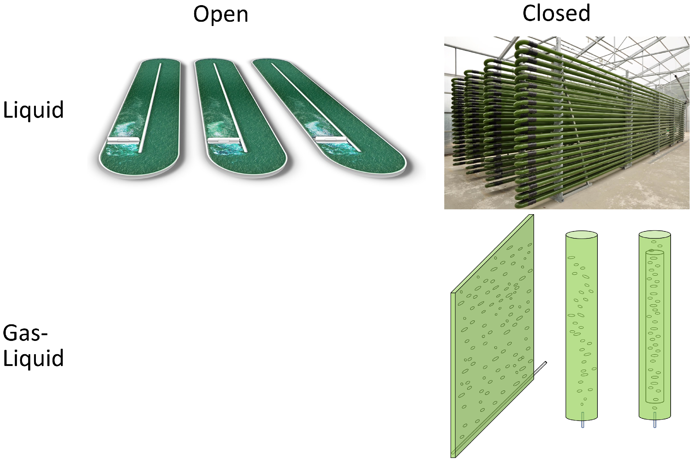
A common way of classification is to differentiate between open and closed reactors [5,9]. This classification can be extended by considering the type of fluids in the illuminated part of the reactor, which leads to the classification of typical photobioreactors as being depicted in Figure 1. As the focus of this review is on Computational Fluid Dynamics (CFD), we only consider common reactors for submerged cultures and alternative reactor types, e.g., [53,54,55], are omitted.

The typical design variant of open reactors are Open Raceway Ponds (ORP), see Figure 1, top left. They are characterized by a liquid depth between 20 and 30 cm [58]. The flow in ORP is created by a rotating paddle wheel with a typical flow velocity between 20 and 30 cm s⁻¹ [58,59]. Consequently, the corresponding values of the Reynolds number $Re=uL/\nu$ range roughly between ${10}^4$ and ${10}^5$ and the flow is turbulent. We consider ORP as single-phase reactors even though they have a free surface and carbon dioxide is supplied by sparging CO₂-enriched air into the liquid at certain spots in the reactor. However, this occurs locally and no significant effects of gas sparging on the distribution of light, the flow, mixing or heat transfer must be expected. The assumption of single-phase flow is in line with most models for ORP [22,23,32,33,34,35,43].

Among closed photobioreactors, one finds a much larger variety of designs, see Figure 1, top right and bottom right. Tubular photobioreactors consist of vertically or horizontally aligned tubes having diameters in the order of 5 cm to ensure a large surface-to-volume ratio [14]. Experimental design variants include helical tubular reactors [60] or tubes with static mixers [24,61]. Centrifugal pumps are used to create the a turbulent flow in the tubes, with values of the Reynolds number between 10,000 and 50,000 [14]. For the supply of CO₂ and out-gassing of O₂, one usually finds a connected bubble column or airlift, whose volume is small compared to the tubular solar receiver.

There is a large variety of photobioreactor types where the flow is created pneumatically by sparging gas into the liquid. Among these, the most common designs are Flat-panel airlift (FPA) photobioreactors, bubble column photobioreactors and airlift photobioreactors, see Figure 1, bottom right. Numerous design variants exist for all basic configurations, see e.g., [62,63] or [14,15,16,49,50,51,52]. FPA reactors are characterized by a thickness of 2–3 cm, while bubble column and airlift reactors can have diameters between 5 and 20 cm or even larger. The sparging of the gas in any kind of these reactors can occur via dip tubes, perforated pipes, ring spargers or porous plates [64]. The sparger design as well as the gas flow rate determine the bubble size distribution, the gas hold-up, gas-liquid mass transfer and the overall flow field.

Typical values of the gas flow rate in pneumatically agitated photobioreactors range between 0.5 and 2.5 vvm (gas volume per liquid volume and minute) [65]. Another characteristic operation parameter is the gas superficial velocity $u_g=\dot{V_g}/A_0$ which relates the gas volume flow rate $\dot{V_g}$ to the cross-section $A_0$ of the reactor and typically ranges between ${10}^{-4}$ and ${10}^{-1}$ m s⁻¹ [44,66,67,68,69]. Referring to the flow maps provided by Shah et al. [70] and Zhang et al. [71], one can expect gas-liquid flow in the (pseudo-) homogeneous regime, which is characterized by a narrow bubble size distribution and a small impact of bubble break-up and coalescence. However, one should note that this depends very much on the sparger geometry, and very different bubble size distributions can result at similar gas flow rates for different gas distributors [72]. The bubble shape can be estimated from the Eötvös ($Eo=g\Delta \rho d^2/\sigma$), Reynolds ($Re=\rho du/\mu$) and Morton ($Mo=g{\mu }^4\Delta \rho /{\rho }^2{\sigma }^3$) numbers [73]. This shows a relation between the bubble shape and bubble size, which both affect the interphase forces in two-phase flow.

Finally, it should be stated that little knowledge is available on how the presence of algae cells and their increasing concentration during the cultivation affect the liquid properties and the flow field. Manjrekar et al. [74] estimated an increase of the gas-hold up in microalgae cultures compared to water. Ojha and Al-Dahhan [75] found that the gas hold-up was significantly reduced at high biomass concentration, which they related to a growth-associated increase of the mixture viscosity at constant surface tension. The increase of the dynamic viscosity at higher cell concentration was also reported by other authors [76]. However, as reviewed by Besagni et al. [64], controversial results concerning the effects of viscosity on the bubble column operation characteristics are reported in the literature and further research about this issue will be necessary in future.

2.2. Reaction Environment in Photobioreactors

2.2.1. Light Distribution

Light availability in a photobioreactor is affected by the shape, orientation and emission characteristic of the light source, the geometry and material of the photobioreactor as well as the concentration and radiation characteristics of the cells. There are always spatial gradients of the light intensity due to light-cell interactions, whose strength depends on the local light spectrum and the wavelength-dependency of the cultures’ absorption and scattering characteristics [13]. The absorption spectrum of green algae is usually peaked in the blue and red parts [77,78]. Light at these wavelengths can be completely absorbed after penetrating few millimeters into the culture [79,80]. The relative contribution of green light to the local polychromatic light intensity increases along the light path [26,80] and its weak absorbance causes a flattening of the spatial light intensity gradient [13,81]. In principle, gas bubbles in gas-sparged photobioreactors can scatter light [82,83,84]. However, this becomes insignificant for the light intensity distribution as soon as the biomass concentration increases to concentrations being relevant for industrial production [18].

In simple geometries, light propagation can be treated as a quasi one-dimensional problem, which allows using simple models to achieve fast approximations of the light distribution [4]. In complex geometries, an accurate estimation of the light distribution requires three-dimensional computations [21]. It is also often neglected that reflection or refraction at the various interfaces cause additional heterogeneity of the light intensity distribution and even dark regions may arise in consequence [21,85].

Temporal changes of the light distribution occur due to the evolution of cell density and the adaptation of the pigmentation and cell size [86,87], which determine the radiation characteristics of the cell culture [78,88,89,90]. In case of outdoor cultivation, also the diurnal and seasonal variations of sunlight cause temporal changes of light availability, as they affect the incoming light intensity and possibly the cellular composition [11]. It should also be kept in mind that the optical properties of microalgae cells may vary in time due to the adaption of their intracellular composition [11], see also Section 2.2.1. This uncertainty entails uncertain predictions of the light intensity profiles, and the magnitude of the corresponding errors were found to be of the same order for different light transfer models [13].

2.2.2. Hydrodynamics

The hydrodynamic flow patterns in a photobioreactor mainly depend on its geometry and how the flow is created, i.e., by the pneumatic or mechanical agitation. As discussed in Section 2.1, complex flow patterns can particularly be observed in pneumatically agitated photobioreactors due to the bidirectional and complex interactions between the liquid and gaseous phases.

The hydrodynamics in a photobioreactor affect the growth conditions in submersed cultures in different ways. Hydrodynamic mixing is an important requirement for photobioreactor operations and ensures that all cells within a culture experience similar conditions on average during time scales in the order of the mixing time [66,91]. Looking at shorter time scales, hydrodynamic mixing causes the exposure of cells to a time-dependent fluctuating light intensity, which is claimed to improve the photobioreactor productivity in case that the shuttling of single cells between light and dark zones is synchronized with the time scales of the photosynthetic reaction kinetics [14,92,93,94,95,96,97]. Even though many researchers investigated this “flashing-light effect” [26,95,98,99,100], its practical relevance is still under discussion [26,101,102]. The received temporal light signal is termed the “light regime”, which is defined by the amplitude, frequency and duty cycle of the light intensity fluctuation [100,103,104]. The light regime defines the extend of the flashing-light effect. Its estimation in a given photobioreactor for certain operating conditions requires to consider the light distribution, flow and cell trajectories. This is a complex task, especially in the case of multiphase flows, i.e., in pneumatically agitated photobioreactors. Here, the cell motion is mainly governed by chaotic and non-regular vortices [105,106], and simulating such flows requires the accurate modeling of turbulence and momentum transfer between the gas and liquid phases.

Mixing is not only important for the homogeneous distribution of the cells but also for the convective transport of dissolved gases and nutrients in order to prevent limitations in the culture broth [107]. Related to this is the impact of the flow on the mass transfer of CO₂ and dissolved oxygen across gas-liquid interfaces [66]. The concentration fields of nutrients and dissolved gases are also affected by the kinetics of cellular nutrient consumption, which might be coupled to light absorption [8]. Another aspect to consider is that the shear and tensile stresses associated with mixing must be kept at a low level in order to prevent mechanical cell damage [65,108,109]. Finally, similarly to the mass transfer, the flow patterns affect the heat transfer across the reactor wall [6,110].

2.2.3. Interphase Mass Transfer

The required carbon for photosynthesis is usually supplied by bubbling CO₂-enriched air into the culture [14,111]. An additional need is the outgassing of O₂, which is an inhibitor for the enzyme RubisCo [8,49]. Since the dissolution of CO₂ occurs at gas-liquid interfaces, the dissolved gas must be distributed within the culture volume to be available for photosynthesis. In consequence of the coupled phenomena of interphase mass transfer, transport, light intensity and cellular consumption, concentration gradients of dissolved CO₂ can occur. Including interphase mass transfer in simulation models of photobioreactors can become important, if these gradients lead to local limitations of CO₂ in the culture. In order to determine the relevance of CO₂ limitations and the causing bottlenecks, different dimensionless numbers are available. Regarding the typical operating conditions in photobioreactors (see Section 2.1), one finds for the Reynolds and Peclét numbers $Re=uL/\nu \gg 1$ and $Pe=uL/D\gg 1$, thus, one can safely assume that convection is the dominating transport mechanism for momentum and mass. As an estimate for mass transfer limitations, Garcia-Ochoa et al. [112] propose a modified Damköhler number $Da=GU{R}_{max}/GT{R}_{max}$, where $GU{R}_{max}$ and $GT{R}_{max}$ are the maximum microbial gas uptake rate and the maximum gas transfer rate. The gas transfer rate is related to the Sherwood number $Sh=k_{L}a{d}^2/D$, which can be estimated by means of empirical correlations in terms of $Re$ [112], see also Section 4.6. The maximum gas uptake rate is given by the unlimited microbial gas uptake kinetics with respect to the biomass concentration. For the consumption of CO₂ by microalgae, additional factors as temperature, the chemical state of CO₂ in dependence of pH or carbon concentrating mechanism are of relevance [8].

In case that interphase mass transfer must be included in simulation models, one has to consider that the mass transfer of CO₂ across gas-liquid interfaces depends on the local saturation of dissolved CO₂, the specific interfacial area and the thickness of the liquid boundary layer next to the interface, among others [111]. These quantities again are affected by the convective transport of the solute in the liquid, the hydrodynamic forces acting on the gas-liquid interface as well as the liquid properties. It was shown that the interphase mass transfer in water and microalgae cell cultures can differ due to the effect of the liquid properties on the size and shape of bubbles [74]. Accordingly, simulation models including interphase mass transfer characteristics need to be accurate with regard to the bubble size distribution and the specific interphase area, which depend on both, the sparger type and the flow dynamics due to bubble break-up or coalescence. In order to achieve this, population balance modeling might be employed, see Section 4.5.3. However, this comes at the cost of an increasing model complexity and a higher computational demand. Alternatively, a constant bubble size can be assumed based on an accurate measure of a representative bubble size (e.g., Sauter mean diameter) [64]. For the selection of the most suitable approach, one should consider the flow regime maps [70,71], since they provide an indication at given operating conditions.

2.2.4. Heat Transfer

Heat transfer is another important mechanism that affects the growth conditions in photobioreactors. Heating of the cell culture is mainly due to the absorption of infrared radiation by water [110,113,114]. In comparison to visible light, the absorbance of water is approximately ${10}^3$–${10}^4$ times stronger for near-infrared light and ${10}^4$–${10}^6$ times stronger for the mid and far infrared parts of the spectrum [115]. Therefore, the penetration depth of mid and far infrared radiation in the liquid is in the order of millimeters or even smaller. About 50% of the incident radiation in solar illuminated cultures belongs to the infrared parts of the spectrum making water to be the primary heat-absorbing agent in photobioreactors. Under artificial lightning, the heating of water depends on the type of the light source and the fraction of infrared radiation of the total emitted radiation [116]. Generally, direct or diffuse as well as reflected or ground heat radiation can enter the reactor and contribute to heating [6,110]. Other mechanisms affecting the reactor temperature are the heat transfer over the reactor surface and the convective heat transfer within the culture [110,116,117]. Both phenomena are related to the hydrodynamics in the reactor, since the wall heat transfer depends on the thickness of the hydrodynamic boundary layer. As an additional aspect, evaporation becomes important in open systems with large surface-to-volume ratio [118]. In these cases, simulating the spatial temperature distribution may be part of the design optimization.

When considering heat transfer in CFD simulations of photobioreactors, one should note that different time scales influence how the governing factors change. The incident radiation changes in the course of the diurnal cycle so that characteristic times are found to be in the order of hours. In contrast, the characteristic times scales of the flow and mixing are found to be in the order of seconds to minutes, depending on the reactor type and size [66,117]. Due to this difference in the characteristic times and the very low penetration depth of infrared radiation, one can include radiative heat transfer via boundary conditions in terms of temperature or heat flux [118]. Regarding the short mixing times in photobioreactors with small dimensions, one can even assume an almost homogeneous temperature distribution, which was also confirmed experimentally [119,120]. In this case, it is justified to ignore spatial dependencies and to assume isothermal conditions instead, i.e., excluding heat transfer calculations from CFD models. The situation can be different in tubular photobioreactors, where thermal energy accumulates in flow direction [121], or in open systems with large dimensions [59]. In open systems, thermal radiation is absorbed near the surface while vertical mixing is suppressed with increasing distance from the paddle wheel [59]. Consequently, significant temperature differences may be observed within the culture in dependence of the geometrical (depth, aspect ratio) and operational (paddle wheel speed) parameters [122]. In other words, including heat transfer in CFD simulations of photobioreactors is first and foremost useful if spatial temperature gradients are of interest, while temperature changes in time are typically too slow to capture them with a reasonable computational costs.

3. Overview of CFD Models for Photobioreactors

Table 1 and Table 2 provide an overview of selected Computational Fluid Dynamics (CFD) models for different types of photobioreactors. As a criterion for the selection, we chose the completeness of model description, meaning that all relevant information concerning the modeling was included in the respective papers. We don’t claim the completeness of this listing, as its purpose is to provide a representative overview on the applied approaches, which we discuss in detail hereafter. Besides CFD, a variety of other approaches for modeling photobioreactors exist, e.g., [68,123,124], which, however, are not further considered here regarding the focus of this review.

The purpose of the listed models covers a variety of applications, including the mechanistic understanding of photobioreactors [17,18,19,20,21], investigations on the flashing-light effect [22,23,24,25,26,27,28,29,30,31], photobioreactor design optimization [21,22,29,32,33,34,35,36,37,38,39,40,41,42] and optimization of operating conditions [26,34,35,36,43,44,45]. The different goals of modeling explain why the considered transport phenomena and physical processes differ among the listed works. However, it can also be concluded from Table 1 that no “complete” model that considers all phenomena occurring in photobioreactors was suggested so far.

3.1. Light Transfer

Regarding the modeling of light transfer, Table 1 shows that researchers have chosen different approaches, which will be presented in more detail in Section 4.2. One can mainly distinguish between two approaches: firstly, one-dimensional model equations which enable quick and simple estimates of the light intensity with respect to the distance from the light source [23,24,31,36,39,41,43,125] and secondly, the Radiative Transfer Equation (RTE) [18,26,27,28,34], whose solution requires the application of numerical methods. Besides, some less commonly used models include the application of Lambert-Beers law in 2D [126] or the Diffusion approximation of the RTE [21].

The most prominent model of the first category is Lambert-Beer’s law. There exist also a number of variants as well as several empirical correlations aiming to reflect the shape of light intensity profiles in photobioreactors [127,128]. Although not being listed in Table 1, it should be stated that analytical approximations of the one-dimensional RTE exist, which allow a more accurate consideration of the absorption and scattering characteristics of microalgae cells [129,130,131,132]. This model is known as 2-Flux approximation, or Cornet’s model, see also Section 4.2. Another approach was selected by Gao et al. [30,31], who first computed the full solution of the RTE [133] and used this solution in a second step to derive an empirical correlation for light intensity, which then was employed in their subsequent works. Instead of using simplified or analytical models, some researchers selected the second approach, which is solving the full RTE numerically in one or more dimensions [18,21,26,27,28,34]. This approach is much more challenging concerning the modeling effort and computational demand, even if most CFD codes include modules for radiative transfer calculations, which can also be used to compute light distributions, see also Section 4.2.

In photobioreactors, light is polychromatic and its local intensity is an integral property of the local light spectrum. While most researchers neglect the spectral nature of light, some authors did consider it [18,26,39]. Typically, this is done by computing multiple light distributions, each reflecting the wavelength-specific emission characteristics of the light source and optical properties of the cell culture or, alternatively, representative averaged quantities for a spectral band (gray model). In a second step, the light intensity is calculated by integration over wavelength [84,124].

3.2. Single-Phase Flow

Single-phase flow models were mostly applied for simulating ORP. The rotation of the paddle wheel is considered using the sliding mesh technique [22,32,33,35], where an interface divides the numerical mesh into two parts: one is static while the other one moves with the rotating part at constant velocity. The technique is also routinely used for the simulation of stirred tanks or other geometries with rotating parts [47,48,134].

The turbulent single-phase flow is most commonly modeled with the Reynolds-Averaged-Navier-Stokes (RANS) equations, which balance the mass and momentum of the liquid phase, see Section 4.3.1. Thereby, the effects of the microalgae biomass on the effective density and viscosity of the liquid phase are usually neglected, which is reasonable regarding the typical dry biomass concentrations of the order of 1–10 g/L. In the RANS formulation, the turbulent flow structures are not resolved and the momentum transport due to turbulent fluctuations is expressed in terms of the Reynolds stresses, which requires a turbulence model to derive the turbulent or eddy viscosity. According to Table 1, a number of different turbulence models were employed by researcher: the k-$\epsilon$ model [32,33,43], the RNG k-$\epsilon$ model [22], the realizable k-$\epsilon$ model [35], and the k-$\omega$ models [22,33] are the most commonly used ones. We provide details of these models in Section 4.3.2.

3.3. Multiphase Flow

Due to the variety of pneumatically agitated photobioreactor designs, modeling of gas-liquid flows is an important task. The literature includes models for two-phase gas-liquid flows [17,18,19,25,39,40,41,42,44,45,125,135], solid-liquid flows [21,23,24,34,36,37,38,126] or three-phase gas-solid-liquid flows [19,26,27,28,29,30,31,136]. While the continuous liquid phase is always treated as an Eulerian continuum, the disperse phase(s) is considered either in an Eulerian or Lagrangian sense [137]. The Lagrangian formulation is intuitive since gas bubbles or cells are modeled as discrete objects, which move through the continuous liquid. The equations of motion of each object consider the momentum exchange with the liquid phase via interphase forces. The drawback of this method is its computational expense since a separate equation must be solved for each discrete object. It is easily imaginable that this limits the applicability for gas-liquid flows in case of large bubble columns or airlift photobioreactors, where tens of thousands of bubbles must be resolved [138]. Accordingly, Euler-Lagrange models for gas-liquid flows have been applied only for small scale photobioreactors. The situation is different for cells since their presence has an negligible effect on the liquid flow so that a manageable number of cells as representatives of the culture can be included in a simulation model [24,26].

Table 1. Overview of photobioreactor (PBR) models. Abbreviations are explained at the table bottom.

References	Light Transfer Model 1	Discretization		Flow Phases 2	Multiphase Model 3	Discretization 4		Turbulence 5		Heat Transfer	Mass Transfer	Kinetics 6
Open Raceway Ponds
Hadiyanto et al. [32]	-	-	-	L	-	FVM	3D	RANS	k-$\epsilon$	-	-	-
Park & Li [43]	modified LB	analytical	1D	L	-	FVM	3D	RANS	k-$\epsilon$	-	-	OEM
Yang et al. [22]	-	-	-	L	-	FVM	3D	RANS	RNG k-$\epsilon$	-	-	-
Sawant et al. [33]	-	-	-	L	-	FVM	3D	RANS	k-$\epsilon$	-	-	-
Amini et al. [34]	RTE	DOM	3D	L, S	E-E	FVM	3D	RANS	RNG k-$\epsilon$	ODE	-	OEM
Inostroza et al. [35]	-	-	-	L	-	FVM	3D	RANS	Realizable k-$\epsilon$	-	-	-
Inostroza et al. [35]	-	-	-	L, G	VoF	FVM	3D	RANS	Realizable k-$\epsilon$	-	-	-
Fernandez del Olmo et al. [23]	LB	analytical	1D	L, S	E-L	FVM-DEM	3D	RANS	Realizable k-$\epsilon$	-	-	PSF
Tubular PBR
Perner-Nochta & Posten [24]	Hyperbolic	analytical	1D	L, S	E-L	FVM-DEM	3D	RANS	k-$\epsilon$	-	-	-
Cheng et al. [36]	Hyperbolic	analytical	1D	L, S	E-L	FVM-DEM	3D	RANS	k-$\epsilon$	-	-	-
Gomez-Perez et al. [37]	-	-	-	L, S	E-L	FVM-DEM	3D	RANS	k-$\epsilon$	-	-	-
Gupta [126]	LB	analytical	2D	L, S	E-L	LBM-DEM	3D	DNS		-	-	-
Bubble column PBR
Bitog et al. [44]	-	-	-	L, G	E-L	FVM	3D	RANS	RNG k-$\epsilon$	-	-	-
Bari et al. [17]	-	-	-	L, G	E-L	FVM	3D	RANS	Realizable k-$\epsilon$	ODE	yes	-
Nauha & Alopeus [25,125]	modified LB	analytical	1D	L, G	E-E	FVM	3D	RANS	k-$\epsilon$	-	-	PSF
McHardy et al. [18]	spectral RTE	LBM	3D	L, G	E-E	FVM	3D	RANS	SST	-	-	OEM
Luzi et al. [26]	spectral RTE	LBM	3D	L, G, S	E-E-L	FVM-DEM	3D	RANS	SST	-	-	PSF
Airlift PBR
Luo & Al-Dahhan [136]	-	-	-	L, G, S	E-E-L	FVM-DEM	2D, 3D	RANS	SST	-	-	-
Zhang et al. [38]	-	-	-	L, S	E-L	FVM-DEM	3D	RANS	k-$\epsilon$	-	-	-
Pawar [19]	-	-	-	L, G	E-L	FVM	3D	RANS	k-$\epsilon$	-	-	-
Pawar [19]	-	-	-	L, G, S	E-L-E	FVM	3D	RANS	k-$\epsilon$	-	-	-
Cho & Pott [39]	spectral LB	analytical	1D	L, G	E-E	FVM	2D	not specified		PDE	-	-
Guler et al. [45]	-	-	-	L, G	E-E	FVM	3D	RANS	SST	-	-	-
Teli & Mathpati [135]	-	-	-	L, G	E-E	FVM	3D	RANS	k-$\epsilon$, k-$\omega$, RSM, Realizable k-$\epsilon$	-	-	-
FPA PBR
Wang et al. [40]	-	-	-	L, G	E-E	FVM	3D	RANS	k-$\epsilon$	-	-	-
Loomba et al. [27]	RTE	not specified	1D	L, G, S	E-E-L	FVM-DEM	3D	RANS	k-$\epsilon$	-	-	-
Ali et al. [41]	modified LB	analytical	1D	L, G	E-E	FVM	3D	RANS	k-$\epsilon$	PDE	-	OEM
Hinterholz et al. [42]	-	-	-	L, G	E-E	FVM	2D	RANS	k-$\epsilon$	-	-	-
Li et al. [28]	RTE	DOM	2D	L, G, S	VoF-DEM	LBM	2D	LES	Smagorinsky	-	-	OEM
Others
Pruvost et al. [20]	-	-	-	L	-	FVM	3D	RANS	k-$\omega$	-	-	-
Sato et al. [29]	LB	analytical	1D	L, G, S	E-E-L	FVM-DEM	3D	RANS	k-$\omega$	-	-	Dark reaction
Gao et al. [30]	RTE fit	analytical	1D	L, G, S	E-E-E	FVM	3D	RANS	k-$\omega$	-	-	PSF
Gao et al. [31]	RTE fit	analytical	1D	L, G, S	E-E-L	FVM-DEM	3D	RANS	k-$\omega$	-	-	PSF
Mink et al. [21]	DA	LBM	3D	L, S	E-L	LBM-DEM	3D	LES	Smagorinsky	-	yes	OEM

¹ LB: Lambert-Beer; RTE: Radiative Transfer Equation; DA: Diffusion Approximation, ² L: liquid; G: gaseous; S: solid, ³ E: Eulerian; L: Langrangian, ⁴ FVM: Finite Volume Method; LBM: Lattice Boltzmann method; DOM: Discrete Ordinates method, ⁵ RANS: Reynolds-averaged Navier-Stokes; LES: Large Eddy Simulation; DNS: Direct Numerical Simulation, ⁶ OEM: One-equation model; PSF: Photosynthetic factory model.

Table 1. Overview of photobioreactor (PBR) models. Abbreviations are explained at the table bottom.

References	Light Transfer Model 1	Discretization		Flow Phases 2	Multiphase Model 3	Discretization 4		Turbulence 5		Heat Transfer	Mass Transfer	Kinetics 6
Open Raceway Ponds
Hadiyanto et al. [32]	-	-	-	L	-	FVM	3D	RANS	k-$\epsilon$	-	-	-
Park & Li [43]	modified LB	analytical	1D	L	-	FVM	3D	RANS	k-$\epsilon$	-	-	OEM
Yang et al. [22]	-	-	-	L	-	FVM	3D	RANS	RNG k-$\epsilon$	-	-	-
Sawant et al. [33]	-	-	-	L	-	FVM	3D	RANS	k-$\epsilon$	-	-	-
Amini et al. [34]	RTE	DOM	3D	L, S	E-E	FVM	3D	RANS	RNG k-$\epsilon$	ODE	-	OEM
Inostroza et al. [35]	-	-	-	L	-	FVM	3D	RANS	Realizable k-$\epsilon$	-	-	-
Inostroza et al. [35]	-	-	-	L, G	VoF	FVM	3D	RANS	Realizable k-$\epsilon$	-	-	-
Fernandez del Olmo et al. [23]	LB	analytical	1D	L, S	E-L	FVM-DEM	3D	RANS	Realizable k-$\epsilon$	-	-	PSF
Tubular PBR
Perner-Nochta & Posten [24]	Hyperbolic	analytical	1D	L, S	E-L	FVM-DEM	3D	RANS	k-$\epsilon$	-	-	-
Cheng et al. [36]	Hyperbolic	analytical	1D	L, S	E-L	FVM-DEM	3D	RANS	k-$\epsilon$	-	-	-
Gomez-Perez et al. [37]	-	-	-	L, S	E-L	FVM-DEM	3D	RANS	k-$\epsilon$	-	-	-
Gupta [126]	LB	analytical	2D	L, S	E-L	LBM-DEM	3D	DNS		-	-	-
Bubble column PBR
Bitog et al. [44]	-	-	-	L, G	E-L	FVM	3D	RANS	RNG k-$\epsilon$	-	-	-
Bari et al. [17]	-	-	-	L, G	E-L	FVM	3D	RANS	Realizable k-$\epsilon$	ODE	yes	-
Nauha & Alopeus [25,125]	modified LB	analytical	1D	L, G	E-E	FVM	3D	RANS	k-$\epsilon$	-	-	PSF
McHardy et al. [18]	spectral RTE	LBM	3D	L, G	E-E	FVM	3D	RANS	SST	-	-	OEM
Luzi et al. [26]	spectral RTE	LBM	3D	L, G, S	E-E-L	FVM-DEM	3D	RANS	SST	-	-	PSF
Airlift PBR
Luo & Al-Dahhan [136]	-	-	-	L, G, S	E-E-L	FVM-DEM	2D, 3D	RANS	SST	-	-	-
Zhang et al. [38]	-	-	-	L, S	E-L	FVM-DEM	3D	RANS	k-$\epsilon$	-	-	-
Pawar [19]	-	-	-	L, G	E-L	FVM	3D	RANS	k-$\epsilon$	-	-	-
Pawar [19]	-	-	-	L, G, S	E-L-E	FVM	3D	RANS	k-$\epsilon$	-	-	-
Cho & Pott [39]	spectral LB	analytical	1D	L, G	E-E	FVM	2D	not specified		PDE	-	-
Guler et al. [45]	-	-	-	L, G	E-E	FVM	3D	RANS	SST	-	-	-
Teli & Mathpati [135]	-	-	-	L, G	E-E	FVM	3D	RANS	k-$\epsilon$, k-$\omega$, RSM, Realizable k-$\epsilon$	-	-	-
FPA PBR
Wang et al. [40]	-	-	-	L, G	E-E	FVM	3D	RANS	k-$\epsilon$	-	-	-
Loomba et al. [27]	RTE	not specified	1D	L, G, S	E-E-L	FVM-DEM	3D	RANS	k-$\epsilon$	-	-	-
Ali et al. [41]	modified LB	analytical	1D	L, G	E-E	FVM	3D	RANS	k-$\epsilon$	PDE	-	OEM
Hinterholz et al. [42]	-	-	-	L, G	E-E	FVM	2D	RANS	k-$\epsilon$	-	-	-
Li et al. [28]	RTE	DOM	2D	L, G, S	VoF-DEM	LBM	2D	LES	Smagorinsky	-	-	OEM
Others
Pruvost et al. [20]	-	-	-	L	-	FVM	3D	RANS	k-$\omega$	-	-	-
Sato et al. [29]	LB	analytical	1D	L, G, S	E-E-L	FVM-DEM	3D	RANS	k-$\omega$	-	-	Dark reaction
Gao et al. [30]	RTE fit	analytical	1D	L, G, S	E-E-E	FVM	3D	RANS	k-$\omega$	-	-	PSF
Gao et al. [31]	RTE fit	analytical	1D	L, G, S	E-E-L	FVM-DEM	3D	RANS	k-$\omega$	-	-	PSF
Mink et al. [21]	DA	LBM	3D	L, S	E-L	LBM-DEM	3D	LES	Smagorinsky	-	yes	OEM

¹ LB: Lambert-Beer; RTE: Radiative Transfer Equation; DA: Diffusion Approximation, ² L: liquid; G: gaseous; S: solid, ³ E: Eulerian; L: Langrangian, ⁴ FVM: Finite Volume Method; LBM: Lattice Boltzmann method; DOM: Discrete Ordinates method, ⁵ RANS: Reynolds-averaged Navier-Stokes; LES: Large Eddy Simulation; DNS: Direct Numerical Simulation, ⁶ OEM: One-equation model; PSF: Photosynthetic factory model.

Table 2. Overview of interphase momentum exchange models used for modeling multiphase photobioreactors.

References		Gas-Liquid					Solid-Liquid
	Phases	Drag	Lift	Virtual Mass	Wall Lubrication	Turbulent Dispersion	Drag	Lift	Virtual Mass	Wall Lubrication	Turbulent Dispersion
Bubble column PBR
Nauha & Alopeus [25]	L, G	Schiller-Naumann	-	-	-	-	-	-	-	-	-
Bari et al. [17]	L, G	Schiller-Naumann	-	constant	-	-	-	-	-	-	-
Nauha & Alopeus [125]	L, G	Tomiyama	Tomiyama	-	-	-	-	-	-	-	-
McHardy et al. [18]	L, G	Ishii-Zuber Clift	Legendre-Magnaudet	constant	Frank	Favre-Averaged	-	-	-	-	-
Luzi et al. [26]	L, G, S	Ishii-Zuber Clift	Legendre-Magnaudet	constant	Frank	Favre-Averaged	Schiller-Naumann	-	-	-	-
Airlift PBR
Luo & Al-Dahhan [136]	L, G, S	Schiller-Naumann Ishii-ZuberGrace	neglected	-	-	Lopez de Bertodano	Schiller-Naumann	-	-	-	-
Zhang et al. [38]	L, S	-	-	-	-	-	Morsi-Alexander	-	-	-	-
Pawar [19]	L, G	Schiller-Naummann, Ishii-Zuber, Grace	-	constant	-	-	-	-	-	-	-
Pawar [19]	L, G, S	Schiller-Naummann, Ishii-Zuber, Grace	-	constant	-	-	Schiller-Naumann	Saffmann-Mei	constant	Antal	Favre-Averaged
Guler et al. [45]	L, G	Grace	Legendre-Magnaudet	constant	Frank	Favre-Averaged	-	-	-	-	-
Teli & Mathpati [135]	L, G	Grace	Tomiyama	constant	-	-	-	-	-	-	-
FPA PBR
Loomba et al. [27]	L, G, S	Schiller-Naumann	-	-	-	-	Schiller-Naumann	-	-	-	-
Ali et al. [41]	L, G	Johansen-Boysan	-	-	-	-	-	-	-	-	-
Hinterholz et al. [42]	L, G	Johansen-Boysan	-	-	-	-	-	-	-	-	-
Others
Sato et al. [29]	L, G, S	Schiller-Naumann	constant	constant	-	-	-	-	-	-	-
Gao et al. [30,31]	L, G, S	Tomiyama	constant	constant	Antal	Talvi	Schiller-Naumann	-	-	-	-

Table 2. Overview of interphase momentum exchange models used for modeling multiphase photobioreactors.

References		Gas-Liquid					Solid-Liquid
	Phases	Drag	Lift	Virtual Mass	Wall Lubrication	Turbulent Dispersion	Drag	Lift	Virtual Mass	Wall Lubrication	Turbulent Dispersion
Bubble column PBR
Nauha & Alopeus [25]	L, G	Schiller-Naumann	-	-	-	-	-	-	-	-	-
Bari et al. [17]	L, G	Schiller-Naumann	-	constant	-	-	-	-	-	-	-
Nauha & Alopeus [125]	L, G	Tomiyama	Tomiyama	-	-	-	-	-	-	-	-
McHardy et al. [18]	L, G	Ishii-Zuber Clift	Legendre-Magnaudet	constant	Frank	Favre-Averaged	-	-	-	-	-
Luzi et al. [26]	L, G, S	Ishii-Zuber Clift	Legendre-Magnaudet	constant	Frank	Favre-Averaged	Schiller-Naumann	-	-	-	-
Airlift PBR
Luo & Al-Dahhan [136]	L, G, S	Schiller-Naumann Ishii-ZuberGrace	neglected	-	-	Lopez de Bertodano	Schiller-Naumann	-	-	-	-
Zhang et al. [38]	L, S	-	-	-	-	-	Morsi-Alexander	-	-	-	-
Pawar [19]	L, G	Schiller-Naummann, Ishii-Zuber, Grace	-	constant	-	-	-	-	-	-	-
Pawar [19]	L, G, S	Schiller-Naummann, Ishii-Zuber, Grace	-	constant	-	-	Schiller-Naumann	Saffmann-Mei	constant	Antal	Favre-Averaged
Guler et al. [45]	L, G	Grace	Legendre-Magnaudet	constant	Frank	Favre-Averaged	-	-	-	-	-
Teli & Mathpati [135]	L, G	Grace	Tomiyama	constant	-	-	-	-	-	-	-
FPA PBR
Loomba et al. [27]	L, G, S	Schiller-Naumann	-	-	-	-	Schiller-Naumann	-	-	-	-
Ali et al. [41]	L, G	Johansen-Boysan	-	-	-	-	-	-	-	-	-
Hinterholz et al. [42]	L, G	Johansen-Boysan	-	-	-	-	-	-	-	-	-
Others
Sato et al. [29]	L, G, S	Schiller-Naumann	constant	constant	-	-	-	-	-	-	-
Gao et al. [30,31]	L, G, S	Tomiyama	constant	constant	Antal	Talvi	Schiller-Naumann	-	-	-	-

According to Table 1, the majority of gas-liquid flows is modeled in the Eulerian-Eulerian formulation [18,25,26,27,29,30,31,39,40,41,42,45,125,135,136], thus, as two interpenetrating continua. Only few authors describe the gaseous phase by considering individual bubbles [17,19,44], which might not only be explained by the computational costs, but also by the fact that a realistic Lagrangian description of the complex bubble motion in liquids was just recently achieved [138]. In contrast, microalgae cells are mostly modeled as discrete objects [23,24,26,27,28,29,31,34,36,37,38,136]. Another interesting approach to investigate the kinetics of photosynthesis with regard to mixing-induced light regimes is to employ an Eulerian three-species model for particulate cells [30,139], which reflects the different metabolic states of the microalgae cells according to a photosynthetic factory model [140,141,142], see also Section 4.1.1.

In order to model the interactions between continuous liquid and dispersed bubbles or particles, a number of mechanisms must be considered [137]. Depending on the density ratio between continuous and disperse phase(s), gravity or buoyancy is an important mechanism. Similarly important, drag forces act on moving particles in a continuous liquid. However, there are also other mechanisms to consider. For example, liquid velocity gradients cause the action of lift forces on dispersed particles or bubbles. For small particles as single cells, one-way coupling can be usually assumed [137]. Besides, the magnitude of the lift forces is usually small in comparison to the drag. In that case, the interphase forces can be limited to the consideration of the drag [143]. In case that particles are approximately spherical, the Schiller-Naumann correlation provides a good estimate for the drag coefficient, which is reflected according to Table 1 by its broad usage for modeling cells in photobioreactors [19,26,27,30,40,136].

The situation is different in the case of gas bubbles, which are much larger in size than cells. The lift-induced lateral migration leads to the concentration of large bubbles at the reactor center, while small ones migrate towards walls [144]. The non-uniform distribution of the void fraction causes chaotic flow patterns [145]. Regarding bubble columns, it is well established that vortices appear between the central bubble plume and the column wall [146], which have a significant impact on the mixing of passive tracers like microalgae cells [105]. This example makes clear that the modeling of interphase forces is essential, when models shall be used to investigate the shuttling of cells in photobioreactors and the corresponding light regime. Comparing numerical and experimental results of gas-liquid flows, Masood et al. [147,148] performed a comprehensive analysis of different drag force correlations and examined the influence of interphase forces such as lift, virtual mass, wall lubrication and turbulent dispersion on the flow field. Although there is a general consensus that the complete set of forces should be considered for an accurate description of gas-liquid flows [64], several interface forces are commonly neglected in photobioreactor models.

According to Table 2, the most commonly used drag models for gas-liquid flows are the Schiller-Naumann [17,25,27,29], Grace [45,135], Ishii-Zuber [18,19,26,136] and Tomiyama models [30,31,125], see Section 4.5.2 for details. As discussed before, the Schiller-Naumann model is accurate for spherical rigid objects and therefore should only be used if bubbles are approximately spherical, which is only the case of small bubbles. For distorted bubbles, the Grace model provides a better approximation of the drag coefficient. The Ishii-Zuber model takes not only distorted bubbles into account but also the dense particle effect in bubble swarms. The Tomiyama model provides different correlations with respect to the purity of the gas-liquid mixture. Applied models for the lift coefficient are the Legendre-Magnaudet [18,26] and the Tomiyama [125,135] models. The Tomiyama model computes the lift coefficient with respect to the bubble size and considers also that the direction of lateral migration is different for large and small bubbles. This behavior is considered accurate and therefore recommended [144]. The turbulent dispersion force causes lateral motion and counteracts the lift force effects and pushes large bubbles towards wall regions, while the wall lubrication force counteracts the accumulation of small bubbles near walls by pushing them away [149]. Therefore, all interphase forces must be carefully balanced in order to achieve realistic results [64,148,149]. The comparison makes clear that there a differences between published photobioreactor models and the models being considered as state-of-the-art in the fluid dynamics community.

This accounts similarly for turbulence modeling. The strengths and weaknesses of different turbulence models are comprehensively discussed by Besagni et al. [64], who conclude that the k-$\omega$ SST model leads to a more accurate description of the bubble flow in comparison to the often employed k-$\epsilon$ model [17,19,25,27,38,40,41,42,44,125]. The incorporation of bubble-induced turbulence in turbulence models improves the simulation accuracy, but the development of these models is still objective of recent research [150,151,152] and was not considered in models of photobioreactors.

Concerning the computational costs, it is clear that two-dimensional numerical simulations of multiphase flows require a significantly lower computational time compared to the three-dimensional case. Although it is reported that two-dimensional Eulerian-Eulerian simulations of bubbly flows compare favorably with experiments in terms of time averaged gas-holdup [153], liquid velocity and turbulent kinetic energy [154], they ignore the three-dimensional nature of turbulence [155]. They were found to be highly grid dependent [155] and to predict a frozen plume that does not oscillate, which is due to a too high turbulent viscosity [156,157]. Therefore, although computationally much more expensive, three-dimensional simulations are necessary to obtain a correct determination of the flow field [136,158,159]. It is seen from Table 1 that apart very few models, all photobioreactors models considered 3D flow fields.

3.4. Mass Transfer

Interphase mass transfer models are rarely considered in CFD simulations of photobioreactors and if considered, they are simplified. In Table 1, two examples [17,21] are listed in which mass transfer of dissolved gases were considered. In the work of Bari et al. [17], the gas transfer rate is evaluated in terms of the superficial gas velocity, which, however, is a boundary condition of the simulation. Therefore, no information about interphase mass transfer was directly received from the simulation, though the gas hold-up, which is related to the gas transfer rate [64] was evaluated. In the work of Mink [21], the transport and consumption of dissolved CO₂ in a photobioreactor is modeled with respect to the flow and photosynthetic reaction kinetics. It is assumed that the dissolved gas enters the reactor together with the liquid phase. Since no gas bubbles are simulated, interphase mass transfer also does not take place.

Examples of simulations of the interphase mass transfer of CO₂ in reactive systems are given in [138,160,161,162] for the Euler-Lagrange and Euler-Euler formulations. While in [138,160], the bubble volume was coupled to the change of mass, a constant bubble size was assumed in [161,162], with reasonable agreement to experimental data. In [163] an Euler-Euler modeling framework including a population balance model for the bubble size evolution was presented to calculate the interphase mass transfer in a bubble column. The authors evaluate different models for the mass transfer coefficient and report in all cases good agreements to experimental data. The cited literature provides validated models which can be adopted to photobioreactors in order to include interphase mass transfer in photobioreactor. However, it should be mentioned that the prediction of interphase mass transfer in multiphase flows requires additional equations to be solved. This increases the computational cost, particularly if polydisperse bubble flows are modeled using the population balance equation, see also Section 4.5.3.

3.5. Heat Transfer

Heat transfer is considered in a number of numerical studies on photobioreactors. As discussed in Section 2.2.4, the different time scales of convective mixing and the temporal change of the heat fluxes must be kept in mind. This has two consequences: first, the space dependency is often neglected and second, the coupling of momentum transfer and heat transfer is realized in different ways.

In their study, Bari et al. [17] considered heat transfer from the liquid to gas bubbles. A spatial temperature distribution was achieved indirectly due to the absorption and transport of heat with rising bubbles. This result is valid for time scales of the order of the mixing time. However, most often temperature effects are of interest during a cultivation time of several days. In order to couple CFD simulations of the flow in photobioreactors with variations of the ambient temperature, a possible procedure is to repeat CFD simulations multiple times and update the boundary conditions in between [33]. Finally, there are also examples for spatially resolved simulations of heat transfer in photobioreactors [39,41]. In [39], a balance equation for heat was solved together with the Navier-Stokes equations. Radiative heat transfer was included as a volumetric source term. In [41], first the flow field was solved and then used as an input for solving the energy equation. This procedure corresponds to a one-way coupling without feedback of the temperature on the flow via the temperature-dependency of the material properties. This seems to be justified as the spatial variation of the surface temperature in an ORP with a volume of approximately 10 m³ was found in the order of 5 K.

4. Overview of Submodels for Relevant Phenomena in Photobioreactors

4.1. Growth Kinetics

To capture the dependency of cellular growth on the environmental conditions, a large body of kinetic models has been developed [4,164,165]. We review the most important relationships with specific emphasis on the use of kinetic models in the context of CFD simulations.

4.1.1. Light Dependency of Growth Kinetics

Photosynthesis-Irradiance Relationships

The light-dependent kinetics of photosynthesis and microalgae growth are often modeled by one-equation models which reflect the hyperbolic relationship between light intensity and the rate of photosynthesis P, see Figure 2. Further effects as light inhibition is also considered in some of these models. Usually, a linearly relationship between the rate of photosynthesis and the specific growth rate of the biomass $\mu$ is assumed, thus $\mu \propto P$. We provide some examples of this models in

Table 3. Examples of photosynthesis-irradiance relationship models.

Model	Equation	Reference
Monod (Tamiya)	$\mu ={\mu }_m\frac{I}{K+I}$	[166]
Aiba	$\mu ={\mu }_m\frac{I}{K_1+I+\frac{I^2}{K_2}}$	[167]
Jassby & Platt (Hyperbolic tangent)	$\mu ={\mu }_m\tanh (K·I)$	[168]
Power model	$\mu ={\mu }_m\frac{I^m}{K^m+I^m}$	[169]

. All of these models have the form $\mu ={\mu }_m·f\left(I\right)$. Therefore, the predicted specific growth rate is obtained by scaling the maximum growth rate ${\mu }_m$ with a species-dependent biological function $f\left(I\right)$ that depends on the light intensity, and assumes values between 0 and 1. Thereby, the light intensity I must be specified, and this can be done by using either local or global light intensities, see Section 4.1.1. The empirical constants K are used to fit the respective models to the observed photosynthesis-irradiance relationships.

The characteristic time scale of these models is given by the cellular doubling time ${\mu }^{-1}$, which varies from hours to days, which is much longer than the final times set in CFD simulations. Therefore, the coupling of photosynthesis-irradiance relationships and CFD makes only sense if one aims to investigate the impact of local physical conditions on photosynthesis or cellular growth. Alternatively, one utilizes CFD to calculate the physical growth conditions, while assuming the biological component to be frozen. This is valid due to the very different characteristic time scales of the growth and the flow. The simulation results can then be used by an external solver to update the biomass growth with respect to the outcome of the CFD simulations. This procedure can be performed repeatedly in order to capture cell growth on time scales of whole batches.

Photosynthetic Factory Models

A second class of models aims at predicting the overall photosynthetic reaction kinetics by coupling models for the single reactions, namely light and dark reaction as well as photoinhibition. Although there are different approaches [96], the most common representatives of this class are the photosynthetic factory models, firstly introduced by Eilers and Peeters [140]. The basic assumption behind the photosynthetic factory models is the existence of photosynthetic units (PSU) which can be activated by light absorption. Activated PSU either relax again towards the resting state and drive the dark reaction with the absorbed energy. Alternatively, if light is absorbed in excess, photodamage of activated PSUs transfers them into an inactive state whereby the carried energy is dissipated. Thus, three possible states for PSUs are considered: activated ($x_1$), damaged ($x_2$) or at rest ($x_3$), with $x_i$ being the dimensionless fraction of the total cellular PSUs in the respective state. The transition rates between the single states account for the rates of involved partial reactions and the total rate of photosynthesis, and is usually given by the transition rate from the activated to the resting state.

Figure 3 illustrates the basic principle of the Eilers and Peeters model. According to this scheme, the transition rates of the activated and damaged states are given by the following set of equations

$$x_3=1-x_1-x_2\frac{d{x}_1}{dt}=\alpha I{x}_3-(\beta I+\gamma )x_1\frac{d{x}_2}{dt}=\beta I{x}_1-\delta x_2$$

(1)

where the model parameters $\alpha$, $\beta$, $\gamma$ and $\delta$ account for the kinetic constants of light-dependent activation and damaging of PSU, as well as for their recovery in the photosynthetic dark reaction and by repair, respectively.

Several modifications and extensions of the scheme of Eilers and Peeters were proposed by different authors, taking into account different possibilities for states transitions, different models for the single reaction rates or models accounting for changes in the total number of PSU in order to represent photoacclimation [141,170,171,172,173,174,175,176]. A comparison of the different models including a parameter sensitivity analysis was carried out by Rudnicky et al. [142] showing that all compared models were able to reproduce experimental data although some parameters have little effects on the solution.

The characteristic time scale of photosynthetic factory models governed by the dark reaction rate is in the order of milliseconds, so that they can be resolved in CFD simulations. Because the dynamics of photosynthesis are resolved, photosynthetic factory models are suitable to investigate the effects of fluctuating environmental conditions on the dynamics of photosynthesis, which also includes the investigation of the flashing-light effects on the reactor scale. In practice, there are two ways to realize the coupling, either by a Lagrangian or an Eulerian treatment [26,30,31,139]. In the Lagrangian case, the tracks of representative particles are calculated in the course of the CFD simulation and the corresponding kinetics can be derived in the course of the post-processing from the time-dependent particle position and the local light intensity. In the Eulerian case, the kinetic model is incorporated into the transport equations for each of the resting, activated and damaged states, which are solved together with the flow field [139].

Béchet Classification

Depending on the complexity of a kinetic model, Béchet et al. [4] have introduced a useful classification with three types of models, which was widely adopted [6,177,178,179,180,181].

Type 1 models use only the incident or the average light intensity $I_0$ or $I_{ave}$ as the information source to predict the specific growth rate by means of a photosynthetic-irradiance relationship (Section 4.1.1), and the specific growth rate is modeled as a function $\mu =f\left(I_0\right)$ or $\mu =f\left(I_{ave}\right)$. The local light intensity in the culture as well as the motion of cells and the light regime are ignored, and therefore, no models for light propagation and fluid flow are required. Despite the fact that Type 1 models are quite inaccurate, they are also not useful to be combined with CFD since type 1 models only provide global information while gaining local information is at the heart of CFD.

Type 2 models incorporate the local light intensity, which can enter photosynthetic-irradiance relationships (Section 4.1.1) or photosynthetic factory models (Section 4.1.1). They require a light transfer model (Section 4.2) to calculate the local light intensity. The motion of cells is not resolved, what restricts the investigation of light regimes to cases where the source intensity is modeled as a function of time. It is possible to consider absorbed light instead of light intensity [26,124] and therefore the wavelength-dependency of light and the cellular absorption characteristics. The global specific growth rate is obtained by integrating the local growth prediction $\mu =f(I_0,\mathit{x})$ over volume.

Type 3 models consider the temporal variations of the light intensity due to the motion of cells in photobioreactors. This information is usually fed into a photosynthetic factory models since they are suitable to deal with the effects of light fluctuations. Consequently, in numerical investigations on the effects of mixing on photosynthesis usually this class of models is employed. Type 3 models are the most challenging and complex approach, as they require time-dependent information of the light exposure of single cells, which is obtained from the spatio-temporal position of cells in the flow and the local light intensity. Thus, the flow field as well as the light intensity distribution must be calculated.

4.1.2. Temperature Dependency of Growth Kinetics

As for every organism, the growth rate of microalgae depends on the temperature and is positive within the species-dependent range of thermal tolerance [4,182,183]. As discussed in Section 2.2.4, temperature gradients in photobioreactors exists mainly with respect to time rather than space. With regard to the exposure of cells to different temperatures in the course of mixing, two issues must also be considered. First, the acclimation of the cellular metabolism to temperature fluctuations occurs on much longer time scales than mixing ones. Second, the acclimation of cells requires a certain exposure time to the new environment [184,185]. Both observations imply that on time scales of seconds and minutes the temperature dependency of the observable growth rate can be expressed as $\mu \left(T_{ave}\right)$ rather than ${\mu }_{ave}\left(T\right)$. Due to these arguments, including the temperature dependency of growth in a CFD model seems not to be valid or reasonable.

However, when several CFD simulations are conducted sequentially to represent different times during a batch with fluctuating environment, i.e., different temperature, the temperature dependency might play a role. Although being constant for each simulation, the maximum specific growth rate can change between single simulations, thus a parameter ${\mu }_m\left(T_{ave}\right)$ can be used together with a model for the light dependency on growth. To model this effect, several temperature models are available, and they are summarized in the excellent review of Grimaud et al. [183]. The most recommended model is the cardinal temperature one with inflection [186]. It was shown that this model is suitable to capture the temperature-dependency of growth for many microalgae species [186] and that the parameters can be biologically interpreted [183].

4.2. Light Transfer Models

As discussed in Section 3.1 and Section 2.2.1, light transfer in photobioreactors can be calculated with different models. The optical properties of the cell culture enter light transfer models as material parameters. Particularly, the interaction of light and cells is expressed in terms of the absorption coefficient ${\mu }_a$, the scattering coefficient ${\mu }_s$ as well as the anisotropy factor g. The absorption and scattering coefficients are related to the concentration of biomass X via the relations ${\mu }_a=X·A_{abs}$ and ${\mu }_s=X·A_{sca}$, where $A_{abs}$ and $A_{sca}$ are the absorption and scattering cross-sections per unit mass. Furthermore, the reduced scattering coefficient ${\mu }_s^{\prime }={\mu }_s·(1-g)$ scales anisotropic scattering to isotropic scattering. Modeling frameworks that retrieve the optical properties of cells and cell cultures from composition, shape and structure have been proposed in references [78,88,187]. Besides, a large body of measured optical properties is available for several species [77,78,87,89,90,188,189,190,191,192,193].

4.2.1. Lambert’s Law and Modifications

Lambert’s law (also Beer-Lambert’s law, Boguer’s law) is the most prominent and simplest model to calculate the light distribution in photobioreactors [68,123,124,194,195]. It reads

$$I\left(x\right)=I_0\exp (-{\mu }_{a}x)$$

(2)

Herein, $I\left(x\right)$ is the light intensity with respect to the distance x from the light source, which emits light with intensity $I_0$. Lambert’s law assumes that no scattering of light takes place and absorption is the only relevant mechanism affecting the light transfer. It is possible to average $I_{0,\lambda }$ and ${\mu }_{a,\lambda }$ across the spectrum and compute the polychromatic intensity by means of the spectrum-averaged quantities and Equation (2). If the light source emits collimated light or if the extension of the light source is very large, light transfer reduces to a one-dimensional problem. Therefore, Lambert’s law can be considered as a special solution of the RTE, see Section 4.2.2.

Although Lambert’s law is by far the most used model to calculate light transfer in photobioreactors, see Table 1, some authors point out that realistic light intensity profiles are non-exponential even at single wavelengths [79,133]. This deviation is caused by disregarding scattering which occurs naturally in particulate suspensions. However, the effect of scattering was shown to be only relevant at wavelengths apart from the absorption peaks of the biomass [13].

If scattering cannot be neglected, Lambert’s law provides only an acceptable approximation if the suspensions are dilute or if the path length of radiative transfer is small. Under these conditions single scattering of radiation can be expected and its effect on the radiation intensity can be incorporated into the absorption coefficient [196]. Then, the term extinction coefficient should be preferred because it covers the two different mechanisms of light-cell interaction. An example of this approach is given in [169], where the contribution of absorption to extinction is modeled in a linear dependency of the intracellular pigment content while a constant offset accounts for scattering.

Modifications of Lambert’s law have been proposed in order to increase the prediction accuracy and retain a simple analytical model at the same time. Béchet et al. [4] mention some of these models in their comprehensive review. A modification of Lambert’s law targets the exponent in Equation (2) and introduces hyperbolic functions of the biomass concentration or path length [127,128,197] to account for scattering. Another approach is to write Equation (2) in differential form and using fractional derivatives [198]. This approach offers the flexibility to tune the light transfer model in order to match experimental observations of the polychromatic intensity. Although the mentioned models are not difficult to compute, problems may arise with their application as they are based on empirical relations, which restricts their universality and necessitates previous testing of their accuracy for each specific case. Besides, in all these models information propagates just downstream from the source or in other words, the exponential structure of Lambert’s law is accompanied with the assumption of collimated radiation in the whole domain of interest, which is only valid when light absorbance is strong.

4.2.2. Radiative Transfer Equation

The RTE is the most general light transfer model. It is a balance equation for the radiance $L(\mathit{x},\mathit{n},t)$ and takes the interaction with matter by absorption and scattering into account. The RTE can be derived from the Maxwell’s equations [199]. For a non-emitting medium, it reads [200]

$$\frac{\partial L}{c\partial t}+\mathit{n}·\nabla L={\mu }_s\left(-L+\frac{1}{4\pi }{\int }_{4\pi }^{}\mathsf{\Phi }{L}^{\prime }\mathrm{d}{\mathsf{\Omega }}^{\prime }\right)-{\mu }_{a}L$$

(3)

Herein, $\mathit{x}$ is the spatial coordinate, t is the time, $\mathit{n}$ is a unit vector pointing into the direction of light propagation and c is the speed of light. The function $\mathsf{\Phi }$ is the scattering phase function, whose first moment is equal to the anisotropy factor g. For the simulation of light transfer in microalgae cultures the Henyey-Greenstein phase function is frequently applied [18,26,78,84,188,201]. The angular moments of radiance link the solution of the RTE to the light intensity field. The local light intensity $I(\mathit{x},t)$ is given by the zero_th angular moment of radiance.

Radiation sources and the effects of domain boundaries need to be incorporated into boundary conditions. Dirichlet boundary conditions for the radiance L are usually defined to model the emission characteristics of a source [200]. At reflective walls the boundary values are modeled with respect to the impinging radiance [200].

While in earlier publications Lambert’s law and its modifications were frequently applied, researchers recently are more inclined to utilize the RTE to predict light propagation in photobioreactors [26,84,133,196,202], which is justified by its higher accuracy [79,133]. Thereby, solutions of the RTE are obtained in one [79,84], two [133] or three [18,26,133,203] dimensions with different numerical techniques, depending on the complexity of the geometry. Solving the full RTE required much higher computational effort compared to light calculations using Lambert’s law or analytical solutions of the RTE. The reason for the high computational costs of radiative transfer calculations is that numerical schemes as the Discrete Ordinate Method (DOM) require an angular discretization in addition to the discretization of space [115,200]. In order to save computational resources, the angular discretization might be kept coarse, which, however, can lead to significant errors in the computed radiation field, particularly in case of small or diffuse light sources [204,205,206]. An alternative method for radiative transfer calculations is the Monte Carlo method [207,208], which does not suffer from the need of angular discretization, but has the drawback that computations can be very time-consuming for microalgae cultures since the strong absorbance requires many photons to be traced before smooth results are achieved. Recently, lattice Boltzmann methods as another class of methods were developed to solve the Radiative transfer equation [13,21,209,210,211,212] and some models are included in open software codes [213].

Analytical solutions of the RTE exist for one-dimensional problems, see Section 4.2.3. As recent developments in photobioreactor technology include complex geometries with static mixers [24,36] or internal light sources [21,214], employing the full RTE for light transfer calculations becomes increasingly important.

4.2.3. 2-Flux Model

A significant simplification of the RTE is obtained when the angular fluxes aggregates into a forward and backward component. By considering just two fluxes of radiance, the number of spatial dimensions can be reduced from three to one. Cornet et al. [129,131] applied this approximation to light transfer in photobioreactors and derived an analytical solution of the RTE in one dimension under the assumption of isotropic scattering and one-sided light emission. Later, the model was extended to anisotropic scattering in order to account for the scattering characteristics of microalgae cultures [215]. Cornet’s model was widely applied for light transfer in photobioreactors with a quasi one-dimensional geometry [132,216,217,218] and can be considered a good approximation of light transfer in such systems. Extensions also include the consideration of reflective boundaries [216].

4.2.4. Diffusion Approximation

In the hydrodynamic limit, that is, close to the scattering equilibrium of radiance, light transfer is diffusive and can be approximated by the so-called Diffusion Approximation (DA, also P1 Approximation). It is based on a decomposition of the local radiance in an isotropic and an anisotropic part by expanding the radiance in spherical harmonics [163,211]. The derived approximation is plugged into the RTE, of which the zero_th and the first moments are computed. The equation system is closed by assuming isotropy of the radiation pressure. In steady-state, the DA for an absorbing medium reads

$$-\nabla D·\nabla I+{\mu }_{a}I=0$$

(4)

where the diffusion coefficient is given by $D={\left(3({\mu }_a+{\mu }_s)\right)}^{-1}$. In case of anisotropic scattering, the reduced scattering coefficient ${\mu }_s^{\prime }={\mu }_s(1-g)$ must be used instead of ${\mu }_s$ to scale the scattering phase function to isotropic conditions.

Compared to the RTE, the DA is much more convenient to solve because the number of dimensions is reduced and no angular discretization is required. The accuracy of the DA is limited by definition to situations where radiance is almost isotropic, which requires that photons were scattered many times. This condition is particularly violated near sources of collimated radiation [219]. The assumption of radiance close to equilibrium usually does not reflect the conditions in highly absorbing media as microalgae cultures [220]. This is because the strong absorption counteracts the achievement of an equilibrium state, since light is absorbed before being scattered often enough. Another reason is that the forward scattering of light by microalgae [78,84,188,201] leads to characteristic length scales for equilibration in the same order as the geometrical dimensions of photobioreactors. However, it was shown that the DA can be of practical importance when the light source of a photobioreactor is diffuse [21,201] or for modeling special photobioreactors like foam bed reactors where the foam strongly scatters light [221].

4.3. Single Phase Flows and Turbulence

4.3.1. Conservation Equations

The isothermal flow in single phase photobioreactors is governed by the conservation equations for mass and momentum

$$\frac{\partial }{\partial t}\rho +\nabla ·\left(\rho \mathit{u}\right)=0$$

(5)

$$\frac{\partial }{\partial t}\left(\rho \mathbf{u}\right)+\nabla ·\left(\rho \mathbf{u}\mathbf{u}\right)=-\nabla p+\nabla ·\tau +\rho \mathbf{g}$$

(6)

The symbols $\rho$ and $\mathit{u}$ are the density and velocity vector of the liquid phase. The left-hand side of (6) signifies the temporal and the convective acceleration while the right-hand side of (6) includes the pressure gradient, the divergence of the viscous stress tensor and the gravitational acceleration. The stress tensor is defined as

$$\tau ={\mu }_{eff}\left[\nabla \mathit{u}+{\nabla \mathit{u}}^T-\frac{2}{3}I(\nabla ·\mathit{u})\right]$$

(7)

Herein, ${\mu }_{eff}$ is the effective viscosity which accounts for the contribution of the molecular viscosity ${\mu }_l$ and the turbulent one ${\mu }_t$, i.e., ${\mu }_{eff}={\mu }_l+{\mu }_t$. There are many approaches to model the turbulent viscosity, which we present hereafter.

4.3.2. Turbulence Models

Two-Equation Models

Two-equation models are among the most utilized ones in turbulence modeling and are widely employed in engineering analysis and research. In principle, they are complete models in the sense that by providing a transport equation for the turbulent kinetic energy and length scales, they do not require any additional information to solve a specific flow problem. However, they do rely on some fundamental assumptions, say, the turbulent fluctuations are locally isotropic and the turbulent production locally balances the dissipation. The latter implies that the turbulent scales are locally proportional to the scales of the mean flow. The eddy viscosity concept is based on this idea, being the eddy viscosity defined as the proportionality constant between the Reynolds stresses and the mean strain rate. The two commonly used types of models are the k-$\epsilon$ and k-$\omega$ turbulence models, of which several variants exits as outlined below.

The k-$\epsilon$ turbulence models: The equation of the specific turbulent kinetic energy k for each phase may be written as

$$\frac{\partial \left(\rho k\right)}{\partial t}+\frac{\partial \left(\rho k{u}_j\right)}{\partial x_j}=P_k-\epsilon \rho +\frac{\partial }{\partial x_j}\left[\left(\mu +\frac{{\mu }_t}{{\sigma }_k}\right)\frac{\partial k}{\partial x_j}\right]+P_{kb}$$

(8)

The terms on the left-hand side of (8) are the rate of change of the specific turbulent kinetic energy and the first term on the right-hand side is the production, that is, the specific kinetic energy per unit volume that an eddy acquires per unit time because of the presence of the strain rate of the mean flow. The second term on the right-hand side of (8) contains the quantity $\epsilon$ which is called the dissipation rate. The latter denotes the mean rate at which the fluctuating strain rate does work on fluctuating viscous stresses. The third term of the right-hand side of (8) represents the diffusion of the turbulent kinetic energy due to the molecular motion, while the fourth term on the right-hand side of (8) incorporates the triple fluctuating velocity correlation and the pressure fluctuations and it is modeled using the gradient diffusion hypothesis. Finally, the last term on the right-hand side represents the production of the turbulent kinetic energy due to buoyancy. The production term $P_k$ may be written as

$$P_k={\mu }_t\left(\frac{\partial u_i}{\partial x_j}+\frac{\partial u_j}{\partial x_i}\right)\frac{\partial u_i}{\partial x_j}-\frac{2}{3}\rho k\frac{\partial u_k}{\partial x_k}$$

(9)

with the turbulent viscosity ${\mu }_t=C_{\mu }{\rho }_k\frac{k^2}{\epsilon }$. The transport equation for the dissipation rate $\epsilon$ reads

$$\frac{\partial \left(\rho \epsilon \right)}{\partial t}+\frac{\partial \left(\rho \epsilon u_j\right)}{\partial x_j}=C_{\epsilon 1}\epsilon f_{\epsilon 1}-C_{\epsilon 2}\rho f_{\epsilon 2}+\frac{\partial }{\partial x_j}\left[\left(\mu +\frac{{\mu }_t}{{\sigma }_{\epsilon }}\right)\frac{\partial \epsilon }{\partial x_j}\right]+C_{\epsilon 1}\frac{\epsilon }{k}{P}_{\epsilon b}$$

(10)

Analogously to the equation for the specific kinetic energy k, the terms on the left-hand side of (10) represent the rate of change of the dissipation while the first term on the right-hand side of (10) is the production of the dissipation due to the complex interplay between the mean flow and the turbulent fluctuations. The second term on the right-hand side of (10) is the rate of destruction of the dissipation, the third term represents the spatial redistribution of dissipation caused by the viscous diffusion and the fourth one is also the transport of the dissipation determined by turbulent and pressure-velocity fluctuations expressed by the gradient diffusion approach. Finally, the last term of (10) models the buoyancy forces.

Differently from the standard k-$\epsilon$ model, see

Table 4. Overview of different k-$\epsilon$ turbulence models. The listed expressions refer to (8)–(10).

Model	${\mathit{f}}_{\mathit{\epsilon }1}$	${\mathit{f}}_{\mathit{\epsilon }2}$	${\mathit{C}}_{\mathit{\mu }}$	${\mathit{C}}_{\mathit{\epsilon }1}$	${\mathit{C}}_{\mathit{\epsilon }2}$	${\mathit{\sigma }}_{\mathit{k}}$	${\mathit{\sigma }}_{\mathit{\epsilon }}$
Standard [224]	$\frac{P_k}{k}$	$\frac{{\epsilon }^2}{k}$	0.09	1.44	1.92	1	1.3
RNG [222]	$\frac{P_k}{k}$	$\frac{{\epsilon }^2}{k}$	0.085	$1.42+\frac{\eta (1-\frac{\eta }{{\eta }_0})}{1+\beta {\eta }^3}$	1.68	0.7194	0.7194
				with ${\eta }_0=4.38$, $\beta =0.012$,
				$\eta =\frac{Sk}{\epsilon }$, where $S={\left(2S_{ij}{S}_{ij}\right)}^{0.5}$
				and $S_{ij}=\frac{1}{2}\left(\frac{\partial u_i}{\partial x_j}+\frac{\partial u_j}{\partial x_i}\right)$
Realizable [223]	S	$\frac{{\epsilon }^2}{k+\sqrt{\nu \epsilon }}$	$\frac{1}{A_0+A_s{U}^{(*)}\frac{k}{\epsilon }}$ with $A_0=4.0$ and	$\max \left[0.43,\frac{\eta }{5+\eta }\right]$	1.9	1	1.2
			$A_s=\sqrt{6}\cos \left(1/3\arccos \left(\sqrt{6}\frac{S_{ij}{S}_{jk}{S}_{ki}}{{\overline{S}}^3}\right)\right)$
			$\overline{S}=\sqrt{S_{ij}{S}_{ij}}$

, Yakhot et al. [222] employed the renormalization group (RNG) approach with a double scale expansion for the Reynolds stress and production of the dissipation terms to develop a different two-equation turbulence model, that is still based on the decomposition of the velocity field into a mean and a fluctuating part. The result is a two-equation eddy viscosity model that is equal to the previously discussed k-$\epsilon$ model but with different constants. This model shows excellent results for the case of homogeneous shear flow and flow over a backward-facing step. Shih et al. [223] proposed a k-$\epsilon$ eddy viscosity model which satisfies the so-called realizability condition, i.e., the positivity of normal Reynold stresses as well as the Schwarz’s inequality for turbulent shear stresses. The whole model is based on a different formulation of the dissipation rate equation and the eddy viscosity. Numerical predictions show that this model performs better than the standard k-$\epsilon$ model for a variety of benchmark flows, such as rotating homogeneous shear flow, boundary-free shear flow, channel and flat boundary layer flow with and without pressure gradients, and backward-facing step flows.

For multiphase simulations, the mixture k-$\epsilon$ model might be employed. It has been developed considering the regimes of low and high phase fractions and recovers the limit of single-phase form when one of the phases approaches zero. Experimental data of Garnier et al. [225] indicate that if the amount of disperse phase fraction exceeds a limit, say 6%, both phases show the tendency to fluctuate as one single entity. Thereby, in situations of high phase fractions, one set of equations for k and $\epsilon$ could be utilized considering a mixture of the continuous and dispersed phase. The turbulent kinetic energy and the dissipation rate of the dispersed phase are linked to the ones of the continuous phase via relations that depend on the response coefficient Ct, that is, the ratio of the fluctuations of the dispersed phase over those of the continuous one. In turn, the mixture properties are related to those of the dispersed and the continuous phase via volume-weighted equations [226].

The k-$\omega$ turbulence models: Most probably the most significant advantage of the k-$\omega$ formulation is that it does not involve damping functions like the k-$\epsilon$ model, thereby being numerically more robust and simplifying the implementation of boundary conditions [227]. $\omega$ can be regarded as either the rate at which dissipation occurs or the inverse of the time scale at which dissipation takes place. This time scale is mainly determined by the largest eddies and $\omega \propto \frac{\epsilon }{k}$. The equations of k and $\omega$ read [228]

$$\frac{\partial \left(\rho k\right)}{\partial t}+\frac{\partial \left(\rho k{u}_j\right)}{\partial x_j}=P_k-{\beta }_k\rho k\omega +\frac{\partial }{\partial x_j}\left[\left(\mu +\frac{{\mu }_t}{{\sigma }_k}\right)\frac{\partial k}{\partial x_j}\right]+P_{kb}$$

(11)

and

$$\frac{\partial \left(\rho \omega \right)}{\partial t}+\frac{\partial \left(\rho \omega u_j\right)}{\partial x_j}=\gamma \frac{\omega }{k}{P}_k-{\beta }_{\omega }\rho {\omega }^2+\frac{\partial }{\partial x_j}\left[\left(\mu +\frac{{\mu }_t}{{\sigma }_{\omega }}\right)\frac{\partial \omega }{\partial x_j}\right]+P_{\omega b}+f_{\omega }$$

(12)

The $\omega$ equation considers the processes of convection, diffusion, production and destruction analogously as equation (10) for $\epsilon$. The main drawback of the k-$\omega$ model lies in its strong sensitivity to freestream conditions. The turbulent viscosity is highly depending on the value of $\omega$ specified outside of the boundary layer, like, for instance at the inlet [227].

The main idea behind the baseline (BSL) model is to combine the k-$\omega$ with the k-$\epsilon$ model utilizing blending functions $F_1$, see

Table 5. Overview of different k-$\omega$ turbulence models. The listed expressions refer to (11) and (12).

Model	${\mathit{\beta }}_{\mathit{k}}$	${\mathit{\beta }}_{\mathit{\omega }}$	$\mathit{\gamma }$	${\mathit{\sigma }}_{\mathit{\omega }}$	${\mathit{\sigma }}_{\mathit{k}}$	${\mathit{\mu }}_{\mathit{t}}$	${\mathit{f}}_{\mathit{\omega }}$
Standard [228]	0.075	0.09	0.56	2	2	$\rho \frac{k}{\omega }$	0
Baseline (BSL)	Blending of coefficients ${\varphi }_1$, ${\varphi }_2$ of the					$\rho \frac{k}{\omega }$	$2(1-F_1)\frac{\rho }{\omega {\sigma }_{\omega 2}}\frac{\partial k}{\partial x_j}\frac{\partial \omega }{\partial x_j}$ with
	standard k-$\omega$ and k-$\epsilon$ models with						$F_1=\tanh \left({\arg }_1^4\right)$ and
	$\frac{1}{\varphi }=F_1\frac{1}{{\varphi }_1}+(1-F_1)\frac{1}{{\varphi }_2}$ gives coefficient						${\arg }_1=\min \left[\max \left(\frac{\sqrt{k}}{0.09\omega y};\frac{500\nu }{y^2\omega }\right);\frac{4\rho {\sigma }_{\omega 2}k}{C{D}_{k\omega }{y}^2}\right]$
	$\varphi$ of the BSL model.						$C{D}_{k\omega }=\max \left(2\rho {\sigma }_{\omega 2}\frac{1}{\omega }\frac{\partial k}{\partial x_j}\frac{\partial \omega }{\partial x_j};{10}^{-20}\right)$
Shear stress transport (SST)	Similar to BSL model.					$\frac{\rho ak}{\max (a_1\omega ;\mathsf{\Omega }{F}_2)}$ with	$2(1-F_1)\frac{\rho }{\omega {\sigma }_{\omega 2}}\frac{\partial k}{\partial x_j}\frac{\partial \omega }{\partial x_j}$
						$F_2=\tanh \left(\max {\left(2\frac{\sqrt{k}}{0.09\omega y};\frac{500\nu }{\omega y^2}\right)}^2\right)$	$F_1=\tanh \left({\arg }_1^4\right)$ and
							${\arg }_1=\min \left[\max \left(\frac{\sqrt{k}}{0.09\omega y};\frac{500\nu }{y^2\omega }\right);\frac{4\rho {\sigma }_{\omega 2}k}{C{D}_{k\omega }{y}^2}\right]$
							$C{D}_{k\omega }=\max \left(2\rho {\sigma }_{\omega 2}\frac{1}{\omega }\frac{\partial k}{\partial x_j}\frac{\partial \omega }{\partial x_j};{10}^{-20}\right)$

. The former is robust and provides accurate results in the near-wall region while the latter is not sensitive to different freestream conditions. It can be seen that the argument of $F_1$ in Table 5 approaches 0 far away from a solid surface due to the presence of terms that vary inversely with the distance y. Besides, the three arguments of ${\arg }_1$ have a definite purpose. The first one is the ratio of the turbulent scale over y and it assumes a constant value in the logarithmic region and decays to zero toward the edge of the boundary layer. The second and the third ones ensure that $F_1$ is equal to one in the viscous sublayer and approaches zero close to the edge of the boundary layer, for more details see [227]. Although the BSL model removes the strong sensitivity of $\omega$ to freestream conditions and it shows improved predictions compared to the standard k-$\omega$ model, it does not consider the transport of the principal turbulent shear stress. This can be critical in situations of adverse pressure gradient flows, since the production may be significantly larger than the dissipation, as it can be shown from the experimental data of Driver [229]. A remedy to this consists of redefining the eddy viscosity to consider the effects of the transport of the principal turbulent shear stress, as being part of the SST model.

Large Eddy Simulations (LES)

The large-eddy simulation technique is based on the idea to resolve large turbulent scales and model the small ones. This is achieved by filtering the Navier-Stokes equations in the physical space. Thereby, the eddies whose scale is smaller than the filter width are not computed directly and need to be modeled. After filtering the Navier-Stokes equations, a new term arises which is the subgrid-scale (SGS) stress tensor and it includes the effects of the small scales of turbulence [230]. While the large scales of the turbulent flow are solved directly, the small scales are considered by appropriate SGS models. However, the isotropic part of the SGS stress tensor is added to the filtered static pressure and is not modeled. In literature, there are several models to compute the SGS stress tensor and some of them are discussed hereafter, see also Table 6. All of them are based on the subgrid eddy-viscosity concept ${\nu }_{SGS}$. The main difference between RANS and LES modeling is that in the former case the eddy viscosity accounts for all the turbulent scales while in the latter case the eddy viscosity accounts only for the small scales.

The Smagorinsky model is probably the first and the most simple LES model. It is based on an algebraic relation of the SGS eddy-viscosity ${\nu }_{SGS}$ that depends on the so-called Smagorinsky constant $C_S$[231]. The value of the Smagorinsky constant $C_S$ used in LES simulations usually varies between 0.065 and 0.25, since those values provide the best results for a wide range of flows. Thereby, one major drawback of the Smagorinsky model is the value of $C_S$, since it generally depends on the discretization scheme, Reynolds number, and fluid flow. Another major drawback is related to the excessive production of subgrid eddy-viscosity close to the walls, but this is alleviated by implementing damping functions.

Germano et al. [232] proposed a modification to the Smagorinsky model to overcome the arbitrariness of the constant $C_S$. First, they redefined the original filtering operator by calling it grid filter and afterward they defined a new filtering operator called test filter where the width of the test filter is larger than that of the grid filter. The formulation of Germano et al. [232] has several advantages over the Smagorinsky model. First, the resolved turbulent stresses become zero in the case of laminar flow and at solid boundaries. Second, the model is proportional to the cube of the distance from a solid boundary in the near-wall region. Third, the model allows for backscattering, either averaged or localized. The latter represents the energy transfer from the small scales of turbulence to the large ones. In addition, the model is not very sensitive to the ratio between the test to the grid filter [232]. Moreover, numerical results are in good agreement with DNS data for transitional [233] and turbulent channel flow [234].

Lilly [235] proposed the application of a least square technique to minimize the difference between the resolved turbulence stresses and its closure model, trying to minimize the error using a least-square approach. The advantage of the Lilly choice of $C_S$ is that if the denominator vanishes, so it also does the numerator since the test scale strains have to vanish completely. However, the main drawback of the Lilly approach is that the value of $C_S$ may become so large that computations become unstable, and therefore the maximum value of $C_S$ should be limited in a simulation.

Nicoud and Ducros [236] showed that the previous LES models [231,232,235] can be written in a unified form in terms of an operator $\overline{OP}$ that depends on space and time and is only a function of the strain rates. However, this is in contrast with DNS results [237], since they show that the dissipation is localized in turbulent eddies and convergence zones. Differently from the previous models, Nicoud and Ducros [236] defined a new operator $\overline{OP}$ that is invariant with respect to translation and rotation, it can be easily implemented both in structured and unstructured meshes, it depends on both the strain and the rotation rates, and it vanishes at the wall without the aid of neither damping functions nor any dynamic procedure. In addition, both strain and rotation rate of turbulent structures are considered [236]. Nicoud and Ducros [236] defined an LES eddy-viscosity model based on the operator $\overline{OP}$ and called it the Wall-Adapting Local Eddy-viscosity (WALE) model. In the case of shear flows, the invariant of the WALE model vanishes, thereby leading to an amount of energy dissipation that is considerably smaller than that detected in eddies and convergence zones. As a consequence, the eddy-viscosity produced in the case of wall-bounded laminar flow is much smaller than the molecular one and the onset of unstable waves may take place indicating that the WALE model can reproduce the transition from laminar to turbulent flow. Besides, it can be shown by scaling arguments that the WALE model behaves like $y^3$ near a solid wall.

Table 6. Overview on LES turbulence models.

Model	Equations
Smagorinsky [231]	${\nu }_{SGS}={(C_S\Delta )}^2\left|\overline{S}\right|$	$|\overline{S}|=\sqrt{2{\overline{S}}_{ij}{\overline{S}}_{ij}}$
Germano [232]	${\nu }_{SGS}=C{\overline{\Delta }}^2\left|\overline{S}\right|$	$C=-\frac{1}{2}\frac{\langle L_{kl}{\overline{S}}_{kl}\rangle }{{\tilde{\overline{\Delta }}}^2\langle |\tilde{\overline{S}}|{\tilde{\overline{S}}}_{mn}{\overline{S}}_{mn}\rangle -{\overline{\Delta }}^2\langle |\tilde{\overline{S}}|{\tilde{\overline{S}}}_{pq}{\overline{S}}_{pq}\rangle }$
Lilly [235]	same as Germano [232]	$C=\frac{1}{2}\left(\frac{L_{ij}{M}_{ij}}{M_{ij}{M}_{ij}}\right)$
WALE [236]	${\nu }_{SGS}={(C_w\Delta )}^2\frac{{\left({S_{ij}}^d{S_{ij}}^d\right)}^{\frac{3}{2}}}{{\left({\overline{S}}_{ij}{\overline{S}}_{ij}\right)}^{\frac{5}{2}}+{\left({S_{ij}}^d{S_{ij}}^d\right)}^{\frac{5}{4}}}$	${S_{ij}}^d{S_{ij}}^d=\frac{1}{6}(S^2{S}^2+{\mathsf{\Omega }}^2{\mathsf{\Omega }}^2)+\frac{2}{3}{S}^2{\mathsf{\Omega }}^2+2I{V}_{S\mathsf{\Omega }}$
		$S^2={\overline{S}}_{ij}{\overline{S}}_{ij}$,    ${\mathsf{\Omega }}^2={\overline{\mathsf{\Omega }}}_{ij}{\overline{\mathsf{\Omega }}}_{ij}$,   $I{V}_{S\mathsf{\Omega }}={\overline{S}}_{ik}{\overline{S}}_{kj}{\overline{\mathsf{\Omega }}}_{jl}{\overline{\mathsf{\Omega }}}_{li}$
		$C_w^2=C_S^2\frac{\langle \sqrt{2}{({\overline{S}}_{ij}{\overline{S}}_{ij})}^{\frac{3}{2}}\rangle }{〈\left({\overline{S}}_{ij}{\overline{S}}_{ij}\right)\frac{{\left({S_{ij}}^d{S_{ij}}^d\right)}^{\frac{3}{2}}}{{\left({\overline{S}}_{ij}{\overline{S}}_{ij}\right)}^{\frac{5}{2}}+{\left({S_{ij}}^d{S_{ij}}^d\right)}^{\frac{5}{4}}}〉}$ with $C_S=0.18$
DKSGS [238]	${\nu }_T=c_{\nu }{k}_{SGS}^{\frac{1}{2}}\overline{\Delta }$	$\frac{\partial k_{SGS}}{\partial t}+{\overline{u}}_i\frac{\partial k_{SGS}}{\partial x_i}=-{\tau }_{ij}\frac{\partial {\overline{u}}_j}{\partial x_j}-\epsilon +\frac{\partial }{\partial x_i}\left({\nu }_T\frac{\partial k_{SGS}}{\partial x_i}\right)$
		$\epsilon =c_{\epsilon }\frac{k_{SGS}^{\frac{1}{2}}}{\overline{\Delta }}$,   $c_{\nu }$ same as Lilly [235]
		$c_{\epsilon }=\frac{\nu \left(〈\frac{\partial {\overline{u}}_i}{\partial x_j}\frac{\partial {\overline{u}}_i}{\partial x_j}〉-\frac{\partial \widetilde{{\overline{u}}_i}}{\partial x_j}\frac{\partial \widetilde{{\overline{u}}_i}}{\partial x_j}\right)}{\left(\frac{K^{\frac{3}{2}}}{\tilde{\Delta }}-〈\frac{k_{SGS}^{\frac{3}{2}}}{\overline{\Delta }}〉\right)}$
LDKSGS [238]	same as the DKSGS	$c_t=\frac{1}{2}\frac{t_{ij}{\sigma }_{ij}}{{\sigma }_{ij}{\sigma }_{ij}}$,    ${\sigma }_{ij}=-\tilde{\Delta }{\left[\frac{1}{2}(\langle {\overline{u}}_i{\overline{u}}_i\rangle -\widetilde{{\overline{u}}_i}\widetilde{{\overline{u}}_i})\right]}^{\frac{1}{2}}\widetilde{{\overline{S}}_{ij}}$
		$t_{ij}=2c_t\tilde{\Delta }{\left[\frac{1}{2}(\langle {\overline{u}}_i{\overline{u}}_j\rangle -\widetilde{{\overline{u}}_i}\widetilde{{\overline{u}}_j})\right]}^{\frac{1}{2}}{\tilde{S}}_{ij}+\frac{2}{3}{\delta }_{ij}\left[\frac{1}{2}\left(\langle {\overline{u}}_i\overline{u_i}\rangle -\widetilde{{\overline{u}}_i}\widetilde{{\overline{u}}_i}\right)\right]$
		$c_{\epsilon }=\frac{\nu \left(〈\frac{\partial {\overline{u}}_i}{\partial x_j}\frac{\partial {\overline{u}}_i}{\partial x_j}〉-\frac{\partial {\tilde{\overline{u}}}_i}{\partial x_j}\frac{\partial {\tilde{\overline{u}}}_i}{\partial x_j}\right)}{\frac{{\left[\frac{1}{2}(\langle {\overline{u}}_i{\overline{u}}_i\rangle -{\tilde{\overline{u}}}_i{\tilde{\overline{u}}}_i)\right]}^{\frac{3}{2}}}{\tilde{\Delta }}}$

Table 6. Overview on LES turbulence models.

Model	Equations
Smagorinsky [231]	${\nu }_{SGS}={(C_S\Delta )}^2\left|\overline{S}\right|$	$|\overline{S}|=\sqrt{2{\overline{S}}_{ij}{\overline{S}}_{ij}}$
Germano [232]	${\nu }_{SGS}=C{\overline{\Delta }}^2\left|\overline{S}\right|$	$C=-\frac{1}{2}\frac{\langle L_{kl}{\overline{S}}_{kl}\rangle }{{\tilde{\overline{\Delta }}}^2\langle |\tilde{\overline{S}}|{\tilde{\overline{S}}}_{mn}{\overline{S}}_{mn}\rangle -{\overline{\Delta }}^2\langle |\tilde{\overline{S}}|{\tilde{\overline{S}}}_{pq}{\overline{S}}_{pq}\rangle }$
Lilly [235]	same as Germano [232]	$C=\frac{1}{2}\left(\frac{L_{ij}{M}_{ij}}{M_{ij}{M}_{ij}}\right)$
WALE [236]	${\nu }_{SGS}={(C_w\Delta )}^2\frac{{\left({S_{ij}}^d{S_{ij}}^d\right)}^{\frac{3}{2}}}{{\left({\overline{S}}_{ij}{\overline{S}}_{ij}\right)}^{\frac{5}{2}}+{\left({S_{ij}}^d{S_{ij}}^d\right)}^{\frac{5}{4}}}$	${S_{ij}}^d{S_{ij}}^d=\frac{1}{6}(S^2{S}^2+{\mathsf{\Omega }}^2{\mathsf{\Omega }}^2)+\frac{2}{3}{S}^2{\mathsf{\Omega }}^2+2I{V}_{S\mathsf{\Omega }}$
		$S^2={\overline{S}}_{ij}{\overline{S}}_{ij}$,    ${\mathsf{\Omega }}^2={\overline{\mathsf{\Omega }}}_{ij}{\overline{\mathsf{\Omega }}}_{ij}$,   $I{V}_{S\mathsf{\Omega }}={\overline{S}}_{ik}{\overline{S}}_{kj}{\overline{\mathsf{\Omega }}}_{jl}{\overline{\mathsf{\Omega }}}_{li}$
		$C_w^2=C_S^2\frac{\langle \sqrt{2}{({\overline{S}}_{ij}{\overline{S}}_{ij})}^{\frac{3}{2}}\rangle }{〈\left({\overline{S}}_{ij}{\overline{S}}_{ij}\right)\frac{{\left({S_{ij}}^d{S_{ij}}^d\right)}^{\frac{3}{2}}}{{\left({\overline{S}}_{ij}{\overline{S}}_{ij}\right)}^{\frac{5}{2}}+{\left({S_{ij}}^d{S_{ij}}^d\right)}^{\frac{5}{4}}}〉}$ with $C_S=0.18$
DKSGS [238]	${\nu }_T=c_{\nu }{k}_{SGS}^{\frac{1}{2}}\overline{\Delta }$	$\frac{\partial k_{SGS}}{\partial t}+{\overline{u}}_i\frac{\partial k_{SGS}}{\partial x_i}=-{\tau }_{ij}\frac{\partial {\overline{u}}_j}{\partial x_j}-\epsilon +\frac{\partial }{\partial x_i}\left({\nu }_T\frac{\partial k_{SGS}}{\partial x_i}\right)$
		$\epsilon =c_{\epsilon }\frac{k_{SGS}^{\frac{1}{2}}}{\overline{\Delta }}$,   $c_{\nu }$ same as Lilly [235]
		$c_{\epsilon }=\frac{\nu \left(〈\frac{\partial {\overline{u}}_i}{\partial x_j}\frac{\partial {\overline{u}}_i}{\partial x_j}〉-\frac{\partial \widetilde{{\overline{u}}_i}}{\partial x_j}\frac{\partial \widetilde{{\overline{u}}_i}}{\partial x_j}\right)}{\left(\frac{K^{\frac{3}{2}}}{\tilde{\Delta }}-〈\frac{k_{SGS}^{\frac{3}{2}}}{\overline{\Delta }}〉\right)}$
LDKSGS [238]	same as the DKSGS	$c_t=\frac{1}{2}\frac{t_{ij}{\sigma }_{ij}}{{\sigma }_{ij}{\sigma }_{ij}}$,    ${\sigma }_{ij}=-\tilde{\Delta }{\left[\frac{1}{2}(\langle {\overline{u}}_i{\overline{u}}_i\rangle -\widetilde{{\overline{u}}_i}\widetilde{{\overline{u}}_i})\right]}^{\frac{1}{2}}\widetilde{{\overline{S}}_{ij}}$
		$t_{ij}=2c_t\tilde{\Delta }{\left[\frac{1}{2}(\langle {\overline{u}}_i{\overline{u}}_j\rangle -\widetilde{{\overline{u}}_i}\widetilde{{\overline{u}}_j})\right]}^{\frac{1}{2}}{\tilde{S}}_{ij}+\frac{2}{3}{\delta }_{ij}\left[\frac{1}{2}\left(\langle {\overline{u}}_i\overline{u_i}\rangle -\widetilde{{\overline{u}}_i}\widetilde{{\overline{u}}_i}\right)\right]$
		$c_{\epsilon }=\frac{\nu \left(〈\frac{\partial {\overline{u}}_i}{\partial x_j}\frac{\partial {\overline{u}}_i}{\partial x_j}〉-\frac{\partial {\tilde{\overline{u}}}_i}{\partial x_j}\frac{\partial {\tilde{\overline{u}}}_i}{\partial x_j}\right)}{\frac{{\left[\frac{1}{2}(\langle {\overline{u}}_i{\overline{u}}_i\rangle -{\tilde{\overline{u}}}_i{\tilde{\overline{u}}}_i)\right]}^{\frac{3}{2}}}{\tilde{\Delta }}}$

Kim and Menon [238] proposed two dynamic models to compute the SGS eddy-viscosity. They are termed Dynamic k-Equation Subgrid Scale (DKSGS) and Local Dynamic k-Equation Subgrid Scale (LDKSGS) model, respectively. They are both based on the formulation of a transport equation for the SGS kinetic energy $k_{SGS}$ and a simple algebraic relationship for the dissipation term $\epsilon$. Besides, the dynamic modeling is applied to evaluate the coefficients $c_{\nu }$ and $c_{\epsilon }$ arising in the LES eddy-viscosity formulation and the correlation for $\epsilon$, respectively. While the $DKSGS$ is defined using two different SGS stress tensors and dissipation rates, the $LDKSGS$ is defined utilizing three SGS stress tensors and dissipation rates. A comparison of the results obtained with the $DKSGS$, $LDKSGS$, and the Germano et al.’s model with DNS simulations of the Taylor-Green vortex flow show that the $LDKSGS$ model delivers better agreement with DNS compared to the $DKSGS$ and the Germano et al.’s model in terms of skewness, flatness as well as production and dissipation. One of the possible reasons for the better agreement between the $LDKSGS$ model and the DNS results could be the retaining of intermittency effects which are not kept in the $DKSGS$ model.

4.4. Euler-Lagrange Modeling of Multiphase Flows

4.4.1. Equations of Motion

In the Lagrangian formulation, the trajectory of a discrete object (e.g., a particle or bubble) is governed by differential equations for the particle position ${\mathit{x}}_p$ and the linear and angular velocities ${\mathit{u}}_p$ and ${\omega }_p$ [137], whereas the liquid flow field is modeled using the Navier-Stokes equations. The governing differential equations for the motion of the considered object read

$${\dot{\mathit{x}}}_p={\mathit{u}}_p{m}_p{\dot{\mathit{u}}}_p=\sum {\mathit{F}}_{p,i}{I}_p{\dot{\omega }}_p=\sum {\mathit{T}}_p$$

(13)

Herein $m_p$ and $I_p$ are the mass and moment of inertia of the object in question, whereas ${\mathit{F}}_{p,i}$ and ${\mathit{T}}_p$ are the forces and the torque acting on the object. For a description of the relevant interphase forces, we refer to Section 4.5.2.

4.4.2. Euler-Lagrange Modeling of Microalgae Cells

Regarding the motion of microalgae cells in photobioreactors, it can be estimated that most species behave as passive tracers, which do not interact due to the low concentration. The Stokes number $St={\tau }_v/{\tau }_f$ is an estimator for ability of a particle to follow the flow [239]. Therein, ${\tau }_v={\rho }_p{d}_p^2/\left(18{\eta }_l\right)$ measures the particle response time to changes in the flow, while ${\tau }_f=L_c/u_c$ is a characteristic time scale of the flow. The quantities $L_c$ and $u_c$ are characteristic lengths and velocities of the fluid flow in a photobioreactor. Microalgae cells are typically characterized by diameters $d_p$ of the order of micrometers and mass densities ${\rho }_p$ slightly higher than water. Assuming the material properties of a growth medium being similar to water, ${\tau }_v$ can be expected in the order of ${10}^{-7}$ to ${10}^{-8}$ s. According to the conditions provided in Section 2.1, the timescale ${\tau }_f$ is of the order of ${10}^{-1}$ to ${10}^0$ s. Therefore, $St\ll 1$, which means that cells follow the flow passively. Accordingly, the motion of cells is governed by inertia and the action of lift forces and rotation is negligible.

4.4.3. Euler-Lagrange Modeling of Gas-Liquid Flows

Within the framework of the Euler-Lagrange (EL) formulation, every single bubble is computed as a point volume acting under Newtonian dynamic, while the movement of the surrounding fluid is described using the volume-averaged unsteady Navier-Stokes equations. This approach usually yields a higher level of details in the resolution of the fluid flow compared to Eulerian-Eulerian approach and the computational costs are lower than those commonly required for DNS simulations.

One of the earliest contribution can be found in the work by Delnoji et al. [240]. They reported a numerical investigation of the two-phase flow in a bubble column reactor, describing the time-dependent, two-dimensional motion of small gas bubbles in the homogeneous regime. The results of two-dimensional numerical simulations show already a meandering motion of a bubble plume for different gas-superficial velocities. Nevertheless, three-dimensional simulations are required to obtain at least a reasonable match with experimental results.

Weber and Bart [241] simulated the movement of rising bubbles in a liquid medium utilizing an oscillating orientation model instead of computing turbulent eddies behind the bubbles. Besides, they implemented stochastic coalescence and break-up models to evaluate the bubble size distribution. To validate their work, they compared the simulated bubble path with experimental data performed in a cylindrical reactor [242]. Their numerical results are in reasonable agreement with experimental ones in terms of mean and instantaneous values of the vertical velocity component and the ondulated trajectories. In another contribution, Weber and Bart [243] compared the Euler-Euler and the Euler-Lagrange formulation for two-phase flows, stating that the Euler-Lagrange approach may be advantageous over the Euler-Euler one if the number of bubbles does not exceed 40,000. Besides, they recommend to use the Euler-Euler if the gas hold-up is high (>5%) and if the bubble size is small (<4 mm). To compute the interaction among bubbles, they used the Monte-Carlo method that calculates the probability of collision. In case of collision, the authors utilized the model of Coulaloglou and Tavlarides [244] to describe coalescence and break-up phenomena, see Section 4.5.3. In particular, they compared three cases with increasing gas superficial velocity and bubble number in a pseudo two-dimensional bubble column. They found that for low-to moderate values of gas superficial velocity, the results of numerical simulations match well with the experimental results of Diaz et al. [245]. On the contrary, significant deviations are found in case of high values of gas superficial velocity.

In another study, Gruber et al. [246] investigated the impact of different models of break-up and coalescence on the results of numerical simulations. Specifically, they compared the break-up and coalescence model of Coulaloglou and Tavlarides [244] with the Lee et al. [247,248] stochastic one. The comparison between their numerical results and the experiments of Deen et al. [249] shows a good match in terms of time-averaged vertical liquid velocity, axial and lateral fluctuating velocity, and gas hold-up.

Zhou et al. [250] evaluated the local dynamic of a bubble in a bubble swarm using a novel path oscillation model combined with the partially-averaged Navier-Stokes (PANS) equation for the continuous phase. By comparing the results of their simulations with the experimental data of Deen et al. [249], the authors could determine the value of the oscillation amplitude of the path that produces the best agreement with experiments.

Vikhansky and Kraft [251] simulated numerically the flow evolving in a rotating disc contactor (RDC) in a pilot scale. To this end, they solved stochastic ordinary differential equations for each bubble. The instantaneous fluid velocity at the droplet location is composed of the mean velocity component and the random fluctuating one generated by the Langevin model. The characteristic size at the outlet of an RDC is in good agreement with the experimental data of and Bart [252], but the size distribution is wider than the measured one.

In subsequent contributions, mass transfer and chemical reactions have also been incorporated. These works are of particularly importance for photobioreactor modeling. For instance, Darmana et al. [160] utilized a 3D discrete bubble model to investigate the hydrodynamic, mass transfer and chemical reaction in a pseudo two-dimensional gas-liquid bubble column. They modeled the mass transfer rate among bubbles using the surface renewal theory and considered the fraction of a chemical specie utilizing a transport equation for each specie. First the authors validated the hydrodynamic only with the experimental data of Deen et al. [249]. Afterward, the authors investigated the case of CO₂ adsorption in water and the chemisorption of CO₂ into a NaOH solution. In a subsequent manuscript, Darmana et al. [253] applied a parallel algorithm based on a mirror domain technique to their Euler-Lagrange model in a four way coupling. They validated the parallel algorithm with the results of serial simulations, finding that the vertical component of the continuous and dispersed velocity field match very well. Afterward, the authors used their parallel algorithm to investigate the influence of coalescence on the hydrodynamics of a bubble column, finding that coalescence phenomena changes significantly the flow structures, average and instantaneous velocities. Subsequently, Darmana et al. [254] carried out experiments of chemisorption of CO₂ into a NaOH solution to validate their numerical results. Although the model reproduces qualitatively very well the entire process, time-averaged averaged velocities, plume meandering period, and gas hold-up only match well with experiments if mass transfer is neglected. If mass transfer is taken into account, the average bubble size computed numerically is higher compared to the one found experimentally, leading to a higher gas hold-up, higher flow velocities and a shorter meandering period compared to experimental data. Besides, the overall computed mass transfer rate is considerably lower than the one found experimentally, maybe due to inaccuracies of the mass transfer closures.

Jain et al. [255] simulated the absorption of CO₂ in a sodium hydroxide solution in a micro-structured bubble column with multiple wire meshes. They found that the decay of the pH in the reactor with wire meshes is approximately 20% faster compared to the case without any mesh. Besides, the authors found a lower Sauter mean diameter for systems with multiple meshes, since bubbles are sieved.

Taborda and Sommerfeld [138] also simulated numerically the reactive flow in the bubble column set-up utilized by Darmana et al. [254]. To this end, they implemented in an OpenFOAM^® solver a bubble oscillation model based on stochastic generation of eccentricity and motion angle of the bubble. The numerical results are in reasonable agreement with the experimental data of [254] in terms of time averaged gas hold-up, equivalent bubble diameter, time averaged bubble velocity and decrease of pH with time.

4.5. Euler-Euler Formulation of Multiphase Flows

4.5.1. Balance Equations

The Eulerian-Eulerian formulations considers single phases as interpenetrating continua. In the Eulerian-Eulerian formulation, the mass and momentum equations for each phase read

$$\frac{\partial }{\partial t}\left({\rho }_k{\alpha }_k\right)+\nabla ·\left({\rho }_k{\alpha }_k{\mathit{u}}_k\right)=0$$

(14)

where the subscripts $k=L,G$ mean liquid and gas, respectively. The symbols ${\rho }_k$, ${\alpha }_k$ and ${\mathbf{u}}_k$ are the density, volume fraction and velocity vector of each phase, respectively. The momentum equations read

$$\frac{\partial }{\partial t}\left({\rho }_k{\alpha }_k{\mathbf{u}}_k\right)+\nabla ·\left({\rho }_k{\alpha }_k{\mathbf{u}}_k{\mathbf{u}}_k\right)=-{\alpha }_k\nabla p+\nabla ({\alpha }_k\nabla ·{\tau }_k)+{\rho }_k{\alpha }_k\mathbf{g}+{\mathbf{M}}_{s,k}$$

(15)

where $k=L,G$ as well. The left-hand side of (15) represents the temporal and the convective acceleration while the right-hand side of (15) includes the pressure gradient, the divergence of the viscous stress tensor, the gravitational acceleration and the interphase forces, respectively. In the Eulerian-Eulerian formulation both phases share the same pressure field and the stress tensor is defined as

$${\tau }_k={\mu }_{k,eff}\left[\nabla {\mathit{u}}_k+\nabla {{\mathit{u}}_k}^T-\frac{2}{3}I(\nabla {\mathit{u}}_k)\right]$$

(16)

Herein, ${\mu }_{k,eff}$ is the effective viscosity of each phase which accounts for the contribution of the molecular viscosity ${\mu }_{k,Lam}$ and the turbulent one ${\mu }_{k,Turb}$, i.e., ${\mu }_{k,eff}={\mu }_{k,Lam}+{\mu }_{k,Turb}$. The turbulent viscosity in multiphase flows is formulated using the models developed for single phase flows, adding an extra term to take into account the interphase transfer. The last term in (15) represents the interphase forces, say, the momentum exchanged between phases, that is

$${\mathit{M}}_{s,k}={\mathit{M}}_{L,G}=-{\mathit{M}}_{G,L}=\sum _A{\mathit{M}}_{L,G}^A={\mathit{F}}_{L,G}^D+{\mathit{F}}_{L,G}^L+{\mathit{F}}_{L,G}^{VM}+{\mathit{F}}_{L,G}^{WL}+{\mathit{F}}_{L,G}^{TD}$$

(17)

The terms on the right-hand side of (17) represent the drag, lift, virtual mass, wall lubrication and turbulent dispersion forces. Several models of each of those forces will be presented in detail in Section 4.5.2.

4.5.2. Interphase Forces

Drag Force Models

The drag force may be written as

$${\mathit{F}}_{L,G}^D=-\frac{3}{4}{\alpha }_G{\rho }_L\frac{C_D}{d}|{\mathit{u}}_G-{\mathit{u}}_L|({\mathit{u}}_G-{\mathit{u}}_L)$$

(18)

where d is the bubble diameter and $C_D$ represents the drag coefficient.

Different correlations for the drag coefficient $C_D$ are available in the literature, see also

Table 7. Drag coefficient correlations.

Model	Correlation
Schiller-Naumann [256]	$C_D=\left\{\begin{array}{cc}\frac{24(1+0.15R{e}^{0.687})}{Re}\hfill & Re\le 1000\hfill \\ 0.44\hfill & Re>1000\hfill \end{array}\right.$	$Re=\frac{{\rho }_L|{\mathit{u}}_G-{\mathit{u}}_L|d}{{\mu }_L}$
Ishii-Zuber [258]	$C_D\left(\mathrm{sphere}\right)=\frac{24}{R{e}_m}(1+0.15R{e}_m^{0.75})$	$R{e}_m=\frac{{\rho }_L|{\mathit{u}}_G-{\mathit{u}}_L|d}{{\mu }_m}$
	$C_D\left(\mathrm{ellipse}\right)=\frac{2}{3}E{o}^{\frac{1}{2}}{\left\{\frac{1+17.67{\left[f\left({\alpha }_G\right)\right]}^{\frac{6}{7}}}{18.67f\left({\alpha }_G\right)}\right\}}^2$	$Eo=\frac{g\Delta \rho d^2}{\sigma }$
	$C_D\left(\mathrm{cap}\right)=\frac{8}{3}{(1-{\alpha }_G)}^2$	$\frac{{\mu }_m}{{\mu }_L}={\left(1-\frac{{\alpha }_G}{{\alpha }_{GM}}\right)}^{\left(-2.5{\alpha }_{GM}\right)\frac{{\mu }_G+0.4{\mu }_L}{{\mu }_G+{\mu }_L}}$
		$f\left({\alpha }_G\right)=\frac{{\mu }_L}{{\mu }_m}\sqrt{1-{\alpha }_G}$
Grace [73]	$C_D=\frac{4}{3}\frac{gd}{U_T^2}\frac{{\rho }_L-{\rho }_G}{{\rho }_L}$	$U_T=\frac{{\mu }_L}{{\rho }_{L}d}M{o}^{-0.149}(J-0.857)$
		$J=\left\{\begin{array}{cc}0.9H^{0.757}\hfill & 2<H\le 59.3\hfill \\ 3.42H^{0.441}\hfill & H>59.3\hfill \end{array}\right.$
		$H=\frac{4}{3}{E}_O{M}^{-0.149}{\left(\frac{{\mu }_L}{{\mu }_{ref}}\right)}^{-0.14}$
Tomiyama and Zun [257]	$C_D=\max \left\{\min \left[\frac{16}{Re}(1+0.15R{e}^{0.687}),\frac{48}{Re}\right],\frac{8}{3}\frac{Eo}{Eo+4}\right\}$	pure system
	$C_D=\max \left\{\min \left[\frac{24}{Re}(1+0.15R{e}^{0.687}),\frac{72}{Re}\right],\frac{8}{3}\frac{Eo}{Eo+4}\right\}$	slightly contaminated system
	$C_D=\max \left\{\left[\frac{24}{Re}(1+0.15R{e}^{0.687})\right],\frac{8}{3}\frac{Eo}{Eo+4}\right\}$	fully contaminated system
Issa and Rusche [259]	$C_D=C_{D0}f\left({\alpha }_G\right)$	$f\left({\alpha }_G\right)=\exp \left(3.64{\alpha }_G\right)+{\alpha }_G^{0.864}$
Roghair et al. [260]	$C_D=C_{\infty }\left(1+\frac{18{\alpha }_G}{Eo}\right)(1-{\alpha }_G)$

. One of the most basic and widely known correlations for the drag-force coefficient is the Schiller-Naumann model. However, this model is only adequate in the viscous regime, where the bubble shape is approximately spherical [256]. Grace [73] improved the previous correlation of Schiller and Naumann by developing a correlation for the drag-force coefficient which is valid also for distorted bubbles. Tomiyama and Zun [257] proposed three different correlations for the drag force coefficient for pure, slightly contaminated, and contaminated gas-liquid systems, using a simple balance of forces acting on a bubble and several correlations for the terminal rising velocity. Ishii and Zuber [258] considered the dense particle effect in the computation of the drag coefficient utilizing of a mixture viscosity. The drag coefficient assumes different forms depending on the flow regimes, i.e., the viscous $C_D\left(\mathrm{sphere}\right)$, the distorted particle $C_D\left(\mathrm{ellipse}\right)$, and the churn turbulent flow regime $C_D\left(\mathrm{cap}\right)$. Other researchers tried to improve the correlation for the drag force coefficient in cases of a high-volume fraction of the disperse phase. Issa and Rusche [259] proposed a simple correlation for the drag coefficient $C_D$ only by correcting the drag coefficient of a single dispersed element with a correction factor that only considers the dispersed volume fraction and must approach unity as the dispersed phase fraction approaches zero. Specifically, the authors suggested a combination of a power-law and an exponential function. Roghair et al. [260] performed Direct Numerical Simulations (DNS) of rising bubbles using a front-tracking model. They utilized the numerical results to develop a closure for the drag coefficient for values of the volume fractions of the dispersed phase between 5% and 45%.

Lift Force Models

The shear-induced lift force assumes the following form

$${\mathit{F}}_{L,G}^L={\alpha }_G{\rho }_L{C}_L({\mathit{u}}_G-{\mathit{u}}_L)\times (▽\times {\mathit{u}}_L)$$

(19)

In (19) $C_L$ is the lift force coefficient. As far as the lift force coefficient is concerned, two models are mostly used in the literature, see

Table 8. Lift coefficient correlations.

Model	Correlation
Legendre-Magnaudet [261]	$C_L=\sqrt{C_{L,lowRe}^2+C_{L,highRe}^2}$
valid for $0.1\le Re\le 500$ and $0\le Sr\le 1$	$C_{L,lowRe}=\frac{6}{{\pi }^2}{\left(ReSr\right)}^{-\frac{1}{2}}{\mathit{J}}^{\prime }(\epsilon )$	$J^{\prime }\left(\epsilon \right)=\frac{2.255}{{(1+0.2{\epsilon }^{-2})}^{\frac{3}{2}}}$
	$C_{L,highRe}=\frac{1}{2}\left(\frac{1+16R{e}^{-1}}{1+29R{e}^{-1}}\right)$	$\epsilon =\sqrt{\frac{Sr}{Re}}$
Tomiyama [262,264,265]	$C_L=\left\{\begin{array}{cc}\min [0.288\tanh \left(0.121Re\right),f\left(E{o}_d\right)]\hfill & \mathrm{for}E{o}_d<4,\hfill \\ f\left(E{o}_d\right)\hfill & \mathrm{for}4\le E{o}_d\le 10.7\hfill \\ -0.27\hfill & \mathrm{for}E{o}_d>10.7\hfill \end{array}\right.$	$E{o}_d=\frac{g({\rho }_L-{\rho }_G)d_H^2}{\sigma }$
	$f\left(E{o}_d\right)=0.00105E{o}_d^3-0.0159E{o}_d^2-0.0204E{o}_d+0.474$	$d_H=d_V(1+0.163E{o}^{0.757})$

. Legendre and Magnaudet [261] carried out numerical simulations of fluid flow around a spherical bubble in presence of a linear shear flow for a wide range of Reynolds numbers Re and shear rate values $Sr$. They fit the numerical results with a correlation that is valid for both low and high bubble Reynolds numbers. Tomiyama [262] distinguishes between small and large bubbles. On the one hand, small bubbles correlate well with the bubble Reynolds number. On the other hand, the lift coefficient of bubbles of intermediate and large diameters strongly depends on the modified Eötvös number which considers the maximum dimension of a bubble. The change in the sign of the lift force is confirmed both experimentally [262] and numerically [263].

Wall Lubrication Force Models

The wall lubrication force models a hydrodynamic force that drives a bubble away from the wall, due to the pressure difference between the two sides of a bubble. The wall lubrication force may be written as

$${\mathbf{F}}_{L,G}^{WL}=-C_{WL}{\alpha }_G{\rho }_L{\left|{\mathbf{u}}_R\right|}^2{\widehat{\mathbf{n}}}_w$$

(20)

In (20), ${\mathbf{u}}_R$ reads ${\mathbf{u}}_R=({\mathbf{u}}_G-{\mathbf{u}}_L)-[{\widehat{\mathbf{n}}}_w·({\mathbf{u}}_G-{\mathbf{u}}_L)]{\widehat{\mathbf{n}}}_w$ and $C_{WL}$ is the wall lubrication force coefficient, see

Table 9. Wall lubrication force coefficient correlations. Note that in the model of Tomiyama the wall lubrication force is differently defined as in (20).

Model	Correlation
Antal et al. [266]	$C_{WL}=\frac{C_{W1}}{d_b}+\frac{C_{W2}}{y_W}$	$C_{W1}=-0.06\left|{\mathbf{u}}_R\right|-0.104$
		$C_{W2}=0.147$
Tomiyama [267]	${\mathbf{F}}_{L,G}^{WL}=-C_{WL}\frac{d_b}{2}\left[\frac{1}{y^2}-\frac{1}{{(D-y)}^2}\right]{\rho }_L{|({\mathbf{u}}_G-{\mathbf{u}}_L)·{\mathbf{n}}_a|}^2{\mathbf{n}}_r$
	$C_{WL}=\left\{\begin{array}{cc}\exp (-0.933Eo+0.179)\hfill & \mathrm{for}1\le Eo\le 5,\hfill \\ 0.007Eo+0.04\hfill & \mathrm{for}5<Eo\le 33\hfill \end{array}\right.$
Frank et al. [264]	$C_{WL}=C_{W3}\left(Eo\right)\max \left\{0,\frac{1}{C_{WD}}\frac{1-\frac{y_W}{C_{WC}{d}_b}}{y_W{\left(\frac{y_W}{C_{WC}{d}_b}\right)}^{p-1}}\right\}$	$C_{W3}=\left\{\begin{array}{cc}\exp (-0.933Eo+0.179)\hfill & \mathrm{for}1\le Eo\le 5,\hfill \\ 0.00599Eo-0.0187\hfill & \mathrm{for}5<Eo\le 33\hfill \\ 0.179\hfill & \mathrm{for}Eo>33\hfill \end{array}\right.$

. Regarding the wall lubrication forces, Antal et al. [266] utilized a two-dimensional approximate solution of the fluid flow between a cylinder and a wall to derive a correlation for the wall force on a sphere. Antal’s model has the drawback that even bubbles located far away from a physical wall get also attracted toward it. Besides, the Antal’s model predicts a wall lubrication force that is too small to counterbalance the lift force arising from the Tomiyama correlation. To cure this problem, Tomiyama [267] proposed a modified wall lubrication force correlation, which depends on the distance to the nearest wall. However, although the Tomiyama formulation improved the previous one by Antal et al., it is still dependent on the reactor diameter. Some of the deficiencies present in the formulations proposed by Antal and Tomiyama have been improved by Frank et al. [264], who proposed a generalized wall lubrication force coefficient that does not consider the pipe diameter as a geometry length scale.

Turbulent Dispersion Forces Models

Turbulent flow in one phase directly affects the migration of fluid particles in other phases. For instance, in gas-liquid two-phase flows, turbulence in the continuous phase is responsible for the migration of bubbles from regions of high concentration to regions of low concentration. This phenomenon is modeled using the turbulent dispersion force. The most common models of turbulent dispersion force are presented in

Table 10. Turbulent dispersion force models.

Model	Correlation
Favre averaged model [268]	${\mathbf{F}}_{G,L,FA}^{TD}=C_{\alpha \beta }\frac{{\nu }_{tL}}{{\sigma }_{tL}}\left(\frac{\nabla \overline{{\alpha }_G}}{\overline{{\alpha }_G}}-\frac{\nabla \overline{{\alpha }_L}}{\overline{{\alpha }_L}}\right)$	$C_{\alpha \beta }=f\left(C_D\right)$
Lopez de Bertodano [269,270,271]	${\mathbf{F}}_{G,L,LB}^{TD}=-C_{TD}{\rho }_L{k}_L\nabla \overline{{\alpha }_L}$	$C_{TD}=C_{\mu }^{\frac{1}{4}}\frac{1}{St(1+St)}$, $C_{\mu }=0.9$
		$C_{TD}=0.1$ or $C_{TD}=0.5$ for ellipsoidal bubbles
Carrica [272]	${\mathbf{F}}_{g,L,CA}^{TD}=-\frac{3}{4}{C}_D\frac{{\alpha }_g{\rho }_L}{N_g{d}_{Bg}}|{\mathit{u}}_g-{\mathit{u}}_L|\frac{{\nu }_L}{S{c}_b}\nabla N_g$	$S_{Cb}=\frac{{\nu }_L}{{\nu }_b}$

and are based on the gradient diffusion hypothesis and averaging techniques. Burns et al. [268] utilized a double time-averaging procedure of the interphase drag term to model the turbulent dispersion forces in multiphase flows. While the Favre averaged [268] and the Lopez de Bertodano model only consider bubbles of the same size, the Carrica’s model [269] has been developed for polydisperse bubbly flows.

4.5.3. Population Balance Equation (PBE)

In a dispersed phase system, the spatial and temporal evolution of a discrete population of bubbles (particles) is modeled by a well-known partial differential equation, the so-called population balance equation (PBE). The PBE is an evolution equation of the number density distribution function (NDF) $n(t,\mathit{x})$ which is related to the number of particles (bubbles) contained in a certain volume V by the following equation

$$N\left(t\right)={\int }_{V}n(t,\mathit{x})\mathrm{d}\mathit{x}$$

(21)

The number density function changes with time and space as a result of interactions within the dispersed or other phases due to continuous phenomena such as convection and diffusion and discontinuous phenomena such as nucleation, aggregation, breakage, and evaporation, only to cite a few. In the case of bubbly flows, in absence of chemical reactions and where only a continuous and a dispersed phase are present, the PBE is usually written as

$$\frac{\partial n(t,\mathit{x})}{\partial t}+\nabla ·\left[n(t,\mathit{x}){\mathit{u}}_G\right]={\mathit{B}}_B-{\mathit{D}}_B+{\mathit{B}}_C-{\mathit{D}}_C$$

(22)

where the terms on the right-hand side of (22) account for the birth rate of smaller bubbles due to break-up of larger ones, the death rate of larger bubbles due to break-up in smaller ones, the birth rate of larger particles due to the coalescence of smaller ones and finally the death rate of particles due to coalescence.

Break-Up Models

Different models for bubble break-up have been developed, which we summarize in Table 11 and discuss hereafter. Generally, the models consist of an expression for the break-up rate as well as a size distribution for the broken bubbles. The feasibility of the different models for photobioreactor modeling must be evaluated by assessing the validity of the respective assumptions for the specific case in question.

Coulaloglou and Tavlarides [244] assume that the deformation and breakage of a drop in a turbulent flow depend on certain parameters, like for instance, drop size, density, surface tension, viscosity, dispersed-phase fraction, and energy dissipation. They proposed a breakage model based on turbulent flow conditions. The turbulent flow is assumed to be locally isotropic, the energy spectrum function is proportional to the power of $-\frac{5}{3}$ to the wavenumber k, viscous effects are negligible, and local pressure fluctuations lead to a drop deformation. The main assumption of their model is that an oscillating drops fragment if the turbulent eddies that hit the fluid particles posseses an amount of kinetic energy greater than the drop surface energy. It is assumed that the droplet sizes formed after the breakage follow a normal density distribution function.

Prince and Blanch [273] use the same idea as Coulaloglou and Tavlarides [244]. However, they report that the model of Coulaloglou and Tavlarides [244] delivers break-up rates that are several orders of magnitude smaller than their experimental results [273]. Prince and Blanch claim that Coulaloglou and Tavlarides did not take the density of the liquid phase into account. Their idea is that bubble breakage occurs due to the interaction between turbulent eddies and bubbles, and they also assume that eddies whose size is equal to or slightly smaller than bubble size can cause the breakage of bubbles. Larger eddies are only responsible for the transport of bubbles and very small eddies do not have enough energy to break bubbles.

Table 11. Overview on selected break-up models for population balance modeling.

Model	Break-Up Rate	Daughter Size Distribution
Luo & Svendsen [274]	${\mathsf{\Omega }}_B\left(v^{\prime }\right)=0.923{\int }_0^{0.5}{\left(\frac{\epsilon }{d^{\prime 2}}\right)}^{\frac{1}{3}}{\int }_{\zeta min}^1\frac{{(1+\zeta )}^2}{{\zeta }^{11/3}}\exp \left(\frac{-12c_f\sigma }{\beta {\rho }_c{\epsilon }^{\frac{2}{3}}{d}^{\prime \frac{5}{3}}{\zeta }^{\frac{11}{3}}}\right)\mathrm{d}\zeta \mathrm{d}{f}_{bv}$	$\eta (v:v{f}_{BV})=\frac{2{\int }_{{\zeta }_{min}}^1{(1+\zeta )}^2{\zeta }^{\frac{-11}{3}}\exp (-{\chi }_C)\mathrm{d}\zeta }{v{\int }_0^1{\int }_{{\zeta }_{min}}^1{(1+\zeta )}^2{\zeta }^{\frac{-11}{3}}\exp (-{\chi }_C)\mathrm{d}\zeta \mathrm{d}{f}_{BV}}$
	${\zeta }_{min}={\lambda }_{min}/d^{\prime }$, ${\lambda }_{min}\sim {({\mu }_l/{\rho }_l)}^{3/4}{\epsilon }^{-1/4}$, $f_{bv}=v^{\prime }/v$
Coulaloglou & Tavlarides [244]	${\mathsf{\Omega }}_B\left(v\right)=C_1{v}^{-\frac{2}{9}}{\epsilon }^{1/3}\exp \left[-\frac{C_2\sigma }{{\rho }_d{v}^{\frac{5}{9}}{\epsilon }^{2/3}}\right]$	$\beta (v^{\prime },v)=\frac{2.4}{v^{\prime }}\exp \left[-4.5\frac{{(2v-v^{\prime })}^2}{v^{\prime 2}}\right]$
Prince & Blanch [273]	${\mathsf{\Omega }}_B\left(v_i\right)={\sum }_e{n}_e{S}_{ie}{({\overline{u}}_{ti}^2+{\overline{u}}_{te}^2)}^{1/2}\exp \left(-\frac{u_{ci}^2}{u_{te}^2}\right)$	as Coulaloglou & Tavlarides
	$S_{ie}=\frac{\pi }{4}{(r_{bi}+r_e)}^{1/2}$, $u_{ci}=1.52{\left(\frac{\sigma }{r_{bi}}\right)}^{1/2}$
Tsouris & Tavlarides [275]	${\mathsf{\Omega }}_B\left(v\right)=0.0118DF\left({\alpha }_G\right){\epsilon }^{1/3}{\int }_{2/d}^{2/d_{e,min}}{\left(\frac{2}{k}+d\right)}^2\times {(8.2k^{-2/3}+1.07d^{2/3})}^{1/2}{k}^2\exp \left[-\frac{E_c}{1.3e}\right]\mathrm{d}k$	$\beta (\delta ,d^{\prime })=\frac{{\epsilon }_{min}+[{\epsilon }_{max}-\epsilon \left(\delta \right)]}{{\int }_0^{d^{\prime }}{\epsilon }_{min}+[{\epsilon }_{max}-\epsilon \left(\delta \right)]\mathrm{d}\delta }$
	$DF\left({\alpha }_G\right)={\left[1+2.5{\alpha }_G\left(\frac{{\mu }_d+0.4{\mu }_c}{{\mu }_d+{\mu }_c}\right)\right]}^2$
Lehr et al. [276]	${\mathsf{\Omega }}_B(v^{\prime },v)=\left\{\begin{array}{cc}{\int }_{d^{\prime }}^d\sqrt{2}C\frac{\sigma }{{\rho }_L{\epsilon }^{1/3}{d}^{\prime 4}}\frac{{(\lambda +d^{\prime })}^2}{{\lambda }^{13/3}}\times \exp \left(-\frac{2\sigma }{{\rho }_L}\frac{1}{{\epsilon }^{2/3}{\lambda }^{2/3}}\frac{1}{d^{\prime }}\right)\mathrm{d}\lambda \hfill & \mathrm{for}0\le v^{\prime }\le v/2\hfill \\ {\mathsf{\Omega }}_B(v-v^{\prime },v)\hfill & \mathrm{for}v/2\le v^{\prime }\le v\hfill \end{array}\right.$	$\beta (v^{*},v^{\prime *})=\left\{\begin{array}{cc}\frac{6}{{\pi }^{3/2}{d}^{\prime *3}}\frac{\exp \left(-\frac{9}{4}{\left[\ln \left(2^{2/5}{d}^{\prime *}\right)\right]}^2\right)}{\left(1+\mathrm{erf}\left[\frac{3}{2}\ln \left(2^{1/15}{d}^{*}\right)\right]\right)}\hfill & \mathrm{for}0\le v^{\prime *}\le v^{*}/2\hfill \\ \beta (v^{*}-v^{\prime *},v^{\prime *})\hfill & \mathrm{for}{v}^{*}/2\le v^{\prime *}\le v^{*}\hfill \end{array}\right.$
Martinez-Bazan et al. [277,278]	${\mathsf{\Omega }}_B\left(d\right)=K_g\frac{\sqrt{\beta \left(\epsilon d^{2/3}\right)-12\sigma /\left(\rho d\right)}}{d}$	$f\left(d^{*}\right)=\frac{[d^{*2/3}-{\Lambda }^{5/3}][{(1-d^{*3})}^{2/9}-{\Lambda }^{5/3}]}{{\int }_{d_{min}^{*}}^{d_{max}^{*}}[d^{*2/3}-{\Lambda }^{5/3}][{(1-d^{*3})}^{2/9}-{\Lambda }^{5/3}]\mathrm{d}\left(d^{*}\right)}$
	$K_g=0.25$	$d^{*}=d_1/d_0$, $\mathsf{\Lambda }=d_c/d_0$
		$d_{min}={[12\sigma /\left(\beta \rho d_0\right)]}^{3/2}{\epsilon }^{-1}$, $d_{max}=d_0{[1-{(d_{min}/d_0)}^3]}^{1/3}$

Table 11. Overview on selected break-up models for population balance modeling.

Model	Break-Up Rate	Daughter Size Distribution
Luo & Svendsen [274]	${\mathsf{\Omega }}_B\left(v^{\prime }\right)=0.923{\int }_0^{0.5}{\left(\frac{\epsilon }{d^{\prime 2}}\right)}^{\frac{1}{3}}{\int }_{\zeta min}^1\frac{{(1+\zeta )}^2}{{\zeta }^{11/3}}\exp \left(\frac{-12c_f\sigma }{\beta {\rho }_c{\epsilon }^{\frac{2}{3}}{d}^{\prime \frac{5}{3}}{\zeta }^{\frac{11}{3}}}\right)\mathrm{d}\zeta \mathrm{d}{f}_{bv}$	$\eta (v:v{f}_{BV})=\frac{2{\int }_{{\zeta }_{min}}^1{(1+\zeta )}^2{\zeta }^{\frac{-11}{3}}\exp (-{\chi }_C)\mathrm{d}\zeta }{v{\int }_0^1{\int }_{{\zeta }_{min}}^1{(1+\zeta )}^2{\zeta }^{\frac{-11}{3}}\exp (-{\chi }_C)\mathrm{d}\zeta \mathrm{d}{f}_{BV}}$
	${\zeta }_{min}={\lambda }_{min}/d^{\prime }$, ${\lambda }_{min}\sim {({\mu }_l/{\rho }_l)}^{3/4}{\epsilon }^{-1/4}$, $f_{bv}=v^{\prime }/v$
Coulaloglou & Tavlarides [244]	${\mathsf{\Omega }}_B\left(v\right)=C_1{v}^{-\frac{2}{9}}{\epsilon }^{1/3}\exp \left[-\frac{C_2\sigma }{{\rho }_d{v}^{\frac{5}{9}}{\epsilon }^{2/3}}\right]$	$\beta (v^{\prime },v)=\frac{2.4}{v^{\prime }}\exp \left[-4.5\frac{{(2v-v^{\prime })}^2}{v^{\prime 2}}\right]$
Prince & Blanch [273]	${\mathsf{\Omega }}_B\left(v_i\right)={\sum }_e{n}_e{S}_{ie}{({\overline{u}}_{ti}^2+{\overline{u}}_{te}^2)}^{1/2}\exp \left(-\frac{u_{ci}^2}{u_{te}^2}\right)$	as Coulaloglou & Tavlarides
	$S_{ie}=\frac{\pi }{4}{(r_{bi}+r_e)}^{1/2}$, $u_{ci}=1.52{\left(\frac{\sigma }{r_{bi}}\right)}^{1/2}$
Tsouris & Tavlarides [275]	${\mathsf{\Omega }}_B\left(v\right)=0.0118DF\left({\alpha }_G\right){\epsilon }^{1/3}{\int }_{2/d}^{2/d_{e,min}}{\left(\frac{2}{k}+d\right)}^2\times {(8.2k^{-2/3}+1.07d^{2/3})}^{1/2}{k}^2\exp \left[-\frac{E_c}{1.3e}\right]\mathrm{d}k$	$\beta (\delta ,d^{\prime })=\frac{{\epsilon }_{min}+[{\epsilon }_{max}-\epsilon \left(\delta \right)]}{{\int }_0^{d^{\prime }}{\epsilon }_{min}+[{\epsilon }_{max}-\epsilon \left(\delta \right)]\mathrm{d}\delta }$
	$DF\left({\alpha }_G\right)={\left[1+2.5{\alpha }_G\left(\frac{{\mu }_d+0.4{\mu }_c}{{\mu }_d+{\mu }_c}\right)\right]}^2$
Lehr et al. [276]	${\mathsf{\Omega }}_B(v^{\prime },v)=\left\{\begin{array}{cc}{\int }_{d^{\prime }}^d\sqrt{2}C\frac{\sigma }{{\rho }_L{\epsilon }^{1/3}{d}^{\prime 4}}\frac{{(\lambda +d^{\prime })}^2}{{\lambda }^{13/3}}\times \exp \left(-\frac{2\sigma }{{\rho }_L}\frac{1}{{\epsilon }^{2/3}{\lambda }^{2/3}}\frac{1}{d^{\prime }}\right)\mathrm{d}\lambda \hfill & \mathrm{for}0\le v^{\prime }\le v/2\hfill \\ {\mathsf{\Omega }}_B(v-v^{\prime },v)\hfill & \mathrm{for}v/2\le v^{\prime }\le v\hfill \end{array}\right.$	$\beta (v^{*},v^{\prime *})=\left\{\begin{array}{cc}\frac{6}{{\pi }^{3/2}{d}^{\prime *3}}\frac{\exp \left(-\frac{9}{4}{\left[\ln \left(2^{2/5}{d}^{\prime *}\right)\right]}^2\right)}{\left(1+\mathrm{erf}\left[\frac{3}{2}\ln \left(2^{1/15}{d}^{*}\right)\right]\right)}\hfill & \mathrm{for}0\le v^{\prime *}\le v^{*}/2\hfill \\ \beta (v^{*}-v^{\prime *},v^{\prime *})\hfill & \mathrm{for}{v}^{*}/2\le v^{\prime *}\le v^{*}\hfill \end{array}\right.$
Martinez-Bazan et al. [277,278]	${\mathsf{\Omega }}_B\left(d\right)=K_g\frac{\sqrt{\beta \left(\epsilon d^{2/3}\right)-12\sigma /\left(\rho d\right)}}{d}$	$f\left(d^{*}\right)=\frac{[d^{*2/3}-{\Lambda }^{5/3}][{(1-d^{*3})}^{2/9}-{\Lambda }^{5/3}]}{{\int }_{d_{min}^{*}}^{d_{max}^{*}}[d^{*2/3}-{\Lambda }^{5/3}][{(1-d^{*3})}^{2/9}-{\Lambda }^{5/3}]\mathrm{d}\left(d^{*}\right)}$
	$K_g=0.25$	$d^{*}=d_1/d_0$, $\mathsf{\Lambda }=d_c/d_0$
		$d_{min}={[12\sigma /\left(\beta \rho d_0\right)]}^{3/2}{\epsilon }^{-1}$, $d_{max}=d_0{[1-{(d_{min}/d_0)}^3]}^{1/3}$

The model of Tsouris and Tavlarides [275] assumes the same form as the one of Prince and Blanch [273]. The eddy-drop collision frequency is based on the assumptions that the isotropic turbulence holds, the drop size is in the inertial sub-range, and only eddies whose size is equal to or smaller than the drop size can cause the breakage of the drops. The main idea underlying the eddy-drop collision frequency is that eddies and drops behave like ideal gas molecules and collision phenomena can be modeled utilizing the kinetic theory of gases. Besides, it is assumed that the energy required for the breakage of a drop is proportional to the energy needed to create a new surface. The daughter drop size distribution should be bimodal with a higher probability density at the ends rather than in the center since the energy requirement for the breakage of a drop into two drops of equal size is larger than the one needed for the breakage into a small and a large drop. Besides, the energy requirement is assumed to be proportional to the new surface area created by the break-up and a minimum drop size for daughter drops is specified.

The model of Luo and Svendsen [274] is based on several assumptions which permit a description of the complex fluid dynamic phenomena typical of break-up processes. Specifically, turbulence is assumed to be isotropic, the breakage of bubbles is assumed to be binary, the breakage volume fraction is assumed to be a stochastic variable, and the energy level of the eddies that hit a bubble determines the occurrence of the break-up. Those assumptions allow writing the bubble breakage as an integral whose kernel is the product between the probability that a particle of size v breaks into two particles and the frequency of eddies. Particle breakage depends not only on the energy contained in the eddies which strike a specific bubble but also on the minimum energy required by the increase of surface area as a result of particle breakup. One of the advantages of the Luo and Svendsen model is that it does not require a correlation for the daughter particle size distribution.

Lehr et al. [276] based their breakage model on the following mechanism of the bubble rupture. First, bubbles deform due to the action of the turbulent flow field. Subsequently, they become stretched in one direction, leading to necking in the shape, and finally, bubbles break. The assumptions used to develop the break-up kernel are that the break-up of bubbles in a turbulent flow field is due to the collision of eddies of different sizes with a bubble, the only binary break-up is considered, the break-up is determined by the balance between interphase forces between liquid and gas and the inertial forces of the eddy that hit a bubble, and only eddies whose size is smaller than the bubble diameter can break it. An advantage of the model of Lehr et al. [276] is that in the case of small bubbles a breakage in two bubbles of equal size has the highest probability, while an unequal size breakage has a higher probability if the size of the bubbles increases.

Haegeaether et al. [279] also start from the Luo and Svendsen [274] break-up model and improved it. The main criticism of the Luo and Svendsen model is that the model is based on the assumption that particle fragmentation occurs when an eddy possesses enough turbulent kinetic energy. This implies that breakage occurs every time an eddy collides with a fluid particle since theoretically there is always a daughter particle that requires less energy than the one that the eddy possesses. This leads to a large and most probably unreasonable number of break-up events, and a number of particle sizes. To remove this deficiency, the authors propose a new breakup criterion based on the energy density and the surface energy criterion. The energy density criterion briefly states that the energy density of an eddy must be higher or at least equal to the energy density of the daughter particles. The new model removes the deficiency of the model of Luo and Svendsen [274] by setting a limit to the minimum size of the daughter particle.

Martínez-Bazán et al. [277,278] developed a model to determine the break-up frequency based on the results of their experiments, conducted to investigate the break-up frequency of bubbles as a function of their size and their critical diameter. Their model assumes that bubbles are injected into a turbulent liquid flow that is locally homogeneous, isotropic, and in equilibrium. The initial size of bubble $d_0$ is assumed to be in the inertial sub-range, the turbulent flow is assumed to be fully developed and the assumption of local isotropy holds. Since the gas volume fraction (${\alpha }_G<{10}^{-5}$) is very small in their experiments, they assumed that only the liquid phase influences the dispersed one and that bubbles undergo a deformation before rupture. Martínez-Bazán et al. [277] also assumed that the rate at which break-up occurs is inversely proportional to the difference between the deformation and the restoring forces which deforms the interface and that the break-up probability is proportional to the difference between the pressure gradient produced by the turbulent fluctuations on a bubble surface and the restoring pressure originated by the surface tension. As far as the probability density function of the daughter bubbles is concerned, they first assumed that after the break-up bubbles fragment into two bubbles of complementary masses. The probability of a parent bubble splitting into two bubbles of equal size is the highest, contrary to several previous models. The present model compares favorably well with their experimental results [278] in terms of daughter probability density function and evolution of the mean Sauter diameter for low and moderate turbulent Weber number. Besides, Martínez-Bazán et al. [278] also consider the possibility of tertiary breakup in case of high turbulent Weber numbers.

The model of Wang et al. [280] is based on the assumptions that only binary break-up is considered, turbulent eddies whose size is equal to or smaller than fluid particles are responsible for their break-up, each eddy has an energy spectrum associated with it due to the turbulent motion, the size of the daughter fluid particles has two constraints, and the binary break-up probability is always the same. Wang et al. [280] point out that Luo and Svendsen’s break-up model possesses two drawbacks from the point of view of the assumptions. The first one is that break-up occurs if the kinetic energy of an eddy is greater than the increase of surface energy that occurs during particle break-up. This assumption may not be entirely valid, especially in cases of a break-up with small fractions where the capillary pressure is high and the radius of curvature is very small. In these cases, although an eddy has kinetic energy higher than the increase of surface energy that happens during the breakup process, it may not have enough dynamic pressure to overcome the capillary one. The second shortcoming is that the probability that a fluid particle breaks with a fraction $f_v$ if an eddy of size $\lambda$ hit it is equal to the probability that an eddy with size $\lambda$ has an amount of kinetic energy larger than the increase of surface energy occurring during the fluid particle break-up. However, if such an eddy with size $\lambda$ satisfies this condition, it may cause all break-ups with a break-up fraction smaller than $f_v$. The authors consider a collision frequency density model similar to that utilized in gas kinetic theory. Besides, they assume that the eddy sizes that contribute to the break-up are within the inertial sub-range so that turbulence can be assumed locally isotropic.

In the model proposed by Andersson and Andersson [281], two criteria need to be fulfilled for the break-up to occur. Those are the energy and the stress criteria. The former asserts that the energy level must be high enough to deform fluid particles. The latter asserts that the stress needs to be maintained over a certain time, so that fluid particles can be stretched sufficiently up to the point of rupture. Bearing those two criteria in mind, the interaction frequency between turbulent eddies and a fluid particle is assumed to be proportional to the volume of a fluid particle. Besides, an eddy must be energetic enough to damage and break a fluid particle during its turnover time.

Coalescence Models

The coalescence rate is modeled as the product of the rate $\Theta$ at which two droplets or bubbles of volume v and $v^{\prime }$ collide and the collision efficiency $\lambda$, which gives the probability that colliding bubbles coalesce, see

Table 12. Overview on selected coalescence models for population balance modeling.

Model	Collision Frequency	Coalescence Efficiency
Coulaloglou & Tavlarides [244]	$\Theta (v,v^{\prime })=c_1(v^{2/3}+v^{\prime 2/3}){(v^{2/9}+v^{\prime 2/9})}^{1/2}{\epsilon }^{1/3}n\left(v\right)n\left(v^{\prime }\right)$	$\lambda (v,v^{\prime })=\exp \left[-\frac{c_2{\mu }_L{\rho }_L\epsilon }{{\sigma }^2}{\left(\frac{v^{1/3}{v}^{\prime 1/3}}{v^{1/3}+v^{\prime 1/3}}\right)}^2\right]$
Tsouris and Tavlarides [275]	$\Theta (d_i,d_j)=\frac{\pi }{4}{(d_i+d_j)}^2{({\overline{u}}_i^2+{\overline{u}}_j^2)}^{1/2}{n}_i{n}_j$ with ${\overline{u}}_i^2=1.07{\epsilon }^{2/3}{d}_i^{2/3}$	$\lambda (d_i,d_j)=\exp \left[-\frac{\overline{T}}{\overline{t}}\right]$ with $\overline{T}=\frac{6\pi {\mu }_L{a}^2}{F_1}\left(1.872\ln \left[\frac{h_1^{1/2}+1.378q}{h_2^{1/2}+1.378q}\right]+0.127\ln \left[\frac{h_1^{1/2}+0.312q}{h_2^{1/2}+0.312q}\right]\right)$
		$q=\frac{a^{1/2}{\mu }_L}{{\mu }_G}$ and $F_1=k_{12}{\rho }_L{\epsilon }^{*2/3}{a}^2{(d_i+d_j)}^{2/3}$
Prince & Blanch [273]	$\Theta (d_i,d_j)={\Theta }^T(d_i,d_j)+{\Theta }^B(d_i,d_j)+{\Theta }^{LS}(d_i,d_j)$	${\lambda }_{d_i,d_j}=\exp \left(-\frac{t_{ij}}{{\tau }_{ij}}\right)$ with $t_{ij}={\left[\frac{r_{ij}^3{\rho }_L}{16\sigma }\right]}^{1/2}\ln \frac{h_o}{h_f}$, $r_{ij}=\frac{1}{2}{\left(\frac{1}{r_i}+\frac{1}{r_j}\right)}^{-1}$ and ${\tau }_{ij}=\frac{r_{ij}^{2/3}}{{\epsilon }^{1/3}}$
	${\Theta }^T(d_i,d_j)=0.089\pi n_i{n}_j{(d_i+d_j)}^2{\epsilon }^{1/3}{(d_i^{2/3}+d_j^{2/3})}^{1/2}$
	${\Theta }^B(d_i,d_j)=n_i{n}_j{S}_{ij}(u_{ri}-u_{rj})$ with $u_{ri}={\left[\frac{2.1\sigma }{{\rho }_L{d}_i}+0.505g{d}_i\right]}^{\frac{1}{2}}$
	${\Theta }^{LS}(d_i,d_j)=n_i{n}_j\frac{4}{3}{(r_i+r_j)}^3\left(\frac{\overline{d{\mathit{u}}_L}}{dr}\right)$
	with ${\mathit{u}}_L=\left(\frac{1-0.75\varphi )}{1-\varphi }\right)\frac{\varphi g{D}_T^2}{48{\nu }_t}\left[1-\frac{r^2}{{\left(\alpha r_T\right)}^2}\right]$ and ${\nu }_t=0.0536\frac{D_T^{1.77}}{{\rho }_L}$
Lehr et al. [276]	$\Theta (d_i,d_j)=\frac{\pi }{4}{(d_i+d_j)}^2{u}^{\prime }$ with $u^{\prime }=\max (\sqrt{2}{\epsilon }^{1/3}\sqrt{d_i^{2/3}+d_j^{2/3}},|{\mathit{u}}_i-{\mathit{u}}_j\left|\right)$	$\lambda =\exp \left[-{\left(\frac{{\alpha }_{max}^{1/3}}{{\alpha }^{1/3}}-1\right)}^2\right]$ with ${\alpha }_{max}=0.6$

.

In the coalescence model of Coulaloglou and Tavlarides [244] it is assumed that colliding droplets must remain in contact for a sufficiently long time, so that the processes of drainage, film rupture, and coalescence may occur. During the coalescence process, turbulent eddies may separate droplets and hinder coalescence. An expression for the collision rate of drops can be formulated assuming locally isotropic turbulent flow and that collisions among drops resemble the collisions among molecules, similar to what happens in the kinetic theory of gases.

Tsouris and Tavlarides [275] proposed a modification of the Coulaloglou and Tavlarides model [244]. They also start by defining the coalescence frequency of drops of different sizes by the product between the drop collision frequency and the coalescence efficiency. To model the coalescence efficiency, the same assumptions of Coulaloglou and Tavlarides [244] are made. Once drops collide, they stay together for some time which is called the contact time, and they either coalesce or bounce away from each other. Coalescence occurs if the contact time is large enough so that the liquid film between two drops drains until a critical thickness is reached. The time needed for the film drainage is called coalescence time.

Prince and Blanch [273] assume that the coalescence of two bubbles in turbulent flows occurs in three steps. First, bubbles collide thereby retaining a small amount of liquid between them. Second, this liquid drains until the thickness of the liquid film that separates the two bubbles reaches a critical value. Finally, bubble coalescence occurs when the liquid film is so thin that it breaks. Collisions of bubbles may occur due to turbulence, buoyancy, and laminar shear. Collision due to turbulence is due to the random motion of bubbles that are transported by the fluctuating turbulent velocity of the liquid phase. Analogously to their breakup model, they assume that only eddies whose size is much larger than the bubble size transport bubbles, while very small eddies do not have sufficient energy to affect bubble motion. Besides, it is also hypothesized that turbulence is isotropic and bubble size lies in the inertial subrange [273]. Collisions due to buoyancy occur since bubbles of different sizes have different velocities. Collisions due to laminar shear occur if bubble columns are operated in the heterogeneous regime, where a circulation profile develops due to the opposite directions of the velocity of the liquid phase. For instance, the velocity of the liquid phase in bubble columns is directed upward in the center of the column and downward close to the walls. Besides, there is also a radial velocity distribution. The fraction of bubble collision that leads to coalescence is determined by the collision efficiency, which depends on the contact time between two bubbles and the time required for bubbles to coalesce.

Wu et al. [282] consider two distinct mechanisms for bubble coalescence, i.e., the random collision-induced bubble coalescence and the wake-entrainment induced bubble coalescence. Random collisions among bubbles are considered to occur only among neighboring bubbles while long-range interactions are discarded.

Hibiki and Ishii [283] considered two mechanisms of bubble coalescence, i.e., the coalescence due to random collisions driven by turbulence and the coalescence due to wake entrainment. To model the coalescence due to random collisions, bubble coalescence is considered to occur due to bubble random collision induced by the turbulence in the liquid phase. To estimate the bubble collision frequency, it is also assumed that bubbles behave like ideal gas molecules in an isotropic turbulent flow field. The authors distinguish two groups of bubbles, one comprising spherical/distorted bubbles (Group I) and another one composed of cap/slug bubbles (Group II). The wake-entrainment bubble induced coalescence is modeled by modifying the original model proposed by Wu et al. [282] and it is extended to spherical/distorted and cap/slug bubbles. When bubbles enter the wake region of a leading cap bubble, they will accelerate and they may collide with the leading one. In situations when either the liquid flow or body forces bring together two bubbles, coalescence may occur. More specifically, when two bubbles approach each other, a film between them forms. This film reduces its size until a small critical thickness is reached. Bubbles move in a continuous phase due to turbulence in that phase, mean-velocity gradients, and buoyancy-induced motion.

Kamp et al. [284] included a coalescence source term in their transport equation for the moment densities. They assumed that if a bubble with diameter $d_i$ coalesces with another bubble of diameter $d_j$ the new formed bubble will have a diameter ${(d_i^3+d_j^3)}^{1/3}$. The bubble interaction process can be divided into two events, that is, separation by collision and film drainage effects. Furthermore, the flow is divided into an external part which is the flow of the continuous phase that brings bubbles together, and an internal part, which is the flow in the liquid film between the surfaces of two approaching bubbles. Kamp et al. [284] postulated that coalescence occurs if the time required for the film drainage from the onset of flattening to film rupture is greater than the interval between the onset of film formation and the moment when bubbles begin to rebound. The authors started their modeling approach by considering the collision of two equal spherical bubbles, approaching each other at equal speed within the limit of a large Reynolds number but a small Weber number. Subsequently, they extended their model to bubbles of different sizes and any Weber number. To model the collision process, they considered a collision between bubbles of different radii that moves with distinct velocities in the horizontal direction in an unbounded liquid at rest, assuming a large collision Reynolds number but a small Weber number. This implies that the radius of the resulting film is much smaller than the radii of the bubbles. Besides, they disregard the work done against viscous dissipation or body forces during the collision and assume the system to be isothermal.

Wang et al. [285] consider three main mechanisms of bubble coalescence which usually take place in gas-liquid systems: coalescence due to turbulent eddies, coalescence due to different bubble rise velocities, and coalescence due to wake entrainment. In literature, often only the coalescence due to turbulent eddies is taken into consideration for simplification. However, this assumption is reasonable only in cases of low and intermediate values of gas superficial velocities, since coalescence due to turbulent eddies is the predominant mechanism of bubble coalescence. Nevertheless, at high values of gas superficial velocity, bubble coalescence due to wake entrainment becomes significant and affects the formation of large bubbles. Besides, also bubble coalescence due to different bubble rise velocities cannot be ignored anymore. As far as the coalescence due to turbulent eddies is concerned, Wang et al. [285] stressed that the formulation of Prince and Blanch [273] presents two main drawbacks: first of all, the ratio of the distance between bubbles and the turbulent path length, which is the distance that a bubble travels due to the turbulent motion, is not considered at all. Second, is the reduction of free space for bubble movement due to the volume occupied by bubbles. If the distance among bubbles is larger than the bubble turbulent path length, the bubble collision frequency is significantly lower than the one predicted by the model of Prince and Blanch [273]. On the contrary, the reduction of the free space among bubbles causes an increase in the bubble collision frequency. To remedy these two shortcomings, they used a corrected formulation of the Luo and Svendsen model [274] for the bubble collision frequency.

Lehr et al. [276] consider the coalescence of more than two bubbles at the same time as a time series of subsequent binary coalescence events. They assume that the coalescence of bubbles occurs in three steps. First, bubbles collide retaining a small amount of liquid between them. Second, the liquid drains until a final critical liquid thickness is reached. Third, coalescence occurs once the final liquid thickness is attained. If the contact time is not sufficiently long, coalescence does not occur and bubbles bounce back. The coalescence kernel is computed as the product between the collision frequency and the coalescence efficiency. Collisions are assumed to arise due to turbulent fluctuations and from the difference in the rising velocity of bubbles of different sizes. In the first case, the characteristic velocity is assumed to be equal to the turbulent eddy velocity with the length scale equal to the bubble size. It is assumed that eddies with bigger sizes only transport bubbles and eddies with smaller sizes do not have sufficient energy to affect bubble motion. In the second case, the characteristic velocity depends on the difference in the rise velocity of bubbles. Collision results in coalescence if two bubbles approach at a relative velocity lower than the critical one. The authors experimentally determined the critical velocity to be $u_{crit}=0.08$ m/s for air-water systems.

PBE Discretization Methods

Population balance equations (PBE) arise in the description of systems containing particles that undergo nucleation, growth, and aggregation and in systems containing bubbles where coalescence and break-up phenomena occur. In most cases, PBEs are completely intractable analytically apart from very specific and idealized situations. Analytical solutions are highly desirable since they perfectly describe how either particles or bubble sizes are distributed in space and time. However, such a degree of detail is often neither required nor justified, since many parameters of the PBE involved in the processes are not known with great accuracy. Moreover, experimental data of size distributions are usually available only for a finite number of size intervals.

An alternative way to solve PBEs analytically is to discretize the particle size distribution (PSD) into a large number of intervals and to solve numerically the resulting equations [286]. This approach can generate sufficiently detailed solutions, although the computational requirements may be significant if the number of intervals increases. A way to overcome this limitation is to discretize the particle size domain only into convenient numbers of intervals to reduce the computational requirements. In one of the earliest models, Hounslow et al. [287] discretized the particle size domain of a PBE using a geometric progression with $\sqrt[3]{2}$ intervals to simulate batches in-vitro kidney stone trials, considering aggregation, growth, and nucleation. First, they compared numerical results with the analytical solutions provided by Gelbard and Seinfeld [288] for the case of a constant coalescence and a size-dependent coalescence kernel. Afterward, they confronted the numerical results with experimental data concerning particle size and moment distributions, finding a very good agreement. Lister et al. [289] extended and improved the previous work of Hounslow et al. [287] using an adjustable discretization of the domain size, that assumes the form of $r_{i+1}/r_i=2^{\frac{1}{q}}$. The choice of a variable discretization is dictated by the fact that a fixed distribution of the size domain is not always desirable, since a fine discretization may be required only in specific ranges. Lister et al. [289] tested the accuracy of their method for different values of q for four different cases, i.e., pure aggregation in a batch vessel, pure aggregation in a continuous stirred tank (CST), nucleation and growth, and pure growth in a batch vessel, and nucleation and growth only in a CST. Comparison between the numerical solutions and the available analytical ones [288,290,291] concerning cumulative oversize number, cumulative volume fraction, moments, and particle size distribution (PSD) indicates that the agreement between them greatly improves by increasing the values of q.

Kumar and Ramkrishna [292] presented a new framework for the discretization of PBEs, considering particle populations in discrete size ranges to be concentrated only in representative volumes. One of the main advantages of this approach is that the coarseness of the discretization can be varied freely, without any specific geometric type, thus having a general and flexible pattern. The technique has been applied to binary and multiple breakages with power-law breakage rates, aggregation with constant, sum, and product kernel, and simultaneous breakage and aggregation. Comparison between analytical [293,294,295] and numerical results show good agreement. Marchal et al. [296] used the CM to simulate the semi-batch crystallization considering the most general case i.e., unsteady state, agglomeration, and breakage of crystals with size-dependent growth rate. The governing PBE has been transformed into a linear system of differential equations by discretizing the range of variation of the crystal size, and the resulting system of differential equations has been solved numerically. Chen et al. [297] simulated the polydisperse two-phase flow in a photobioreactor. They discretized the gas phase into n-classes according to the bubble size and solved together with a two-fluid model in a sequential manner to obtain the local number density for each bubble class. They implemented the discretized equations in two ways using the Algebraic Slip Mixture Model (ASMM). First, they allowed the bubbles to move all at the same velocity, and afterward, they allowed bubbles to move at the characteristic velocity of each bubble class they belong to. Numerical results agree well with experimental ones performed with the CARPT technique. In particular, the results of three-dimensional simulations agree better with experimental ones compared to two-dimensional ones.

Ekambara et al. [298] also simulated the flow pattern in a BC reactor incorporating a PBE with the three-dimensional two-fluid model using the homogeneous multisize group model (MUSIG) to account for the non-uniform bubble size distribution in the flow. The gas hold-up, Sauter mean diameter, axial liquid velocity, turbulent kinetic energy, turbulent dissipation rate, and Reynolds stress have been computed and compared with experimental data at different heights, for the case of the gas superficial velocity of 20 mm/s. Results obtained with the PBE agree better with experimental results compared to the outcomes obtained with uniform bubble size. Nevertheless, the authors set in their simulations that each bubble class travels at the same mean algebraic velocity (homogeneous MUSIG) to reduce the computational time. In general, however, the homogeneous MUSIG problem restricts its applicability to homogeneous disperse flows where the slip velocities of particles are independent of particle size and the particle relaxation time is sufficiently small compared to the inertial time scales. Therefore, it is assumed that the asymptotic slip velocity is attained almost instantaneously, contrarily to the case of bubbly flows in vertical pipes where heterogeneous particle motion become important. Therefore, Krepper et al. [299] developed an inhomogeneous multiple size group (iMUSIG) model and they implemented it in CFX^®. In the inhomogeneous MUSIG model, the gaseous disperse phase is divided into a number N of phases (groups), where each phase is characterized by its velocity field. Moreover, the overall bubble size distribution is represented by dividing the bubble diameter range within each velocity group into several size fractions. The population balance model considering bubble coalescence and break-up is applied to the subsize groups and the mass exchange between the subsize groups can exceed the size ranges assigned to the velocity groups, resulting in mass transfer terms between the different phases or velocity groups. On the one hand, the closure models on bubble forces, that are responsible for bubble migration, agree with experimental observation. On the other hand, clear deviations occur for bubble coalescence and fragmentation, demonstrating that bubble coalescence and break-up phenomena represent a weak point in CFD analysis.

A different approach than the CM is represented by the method of moments (MOM) that traces back its origins from the work of Hulburt and Katz [300]. They formulated a partial differential equation (PDE) for the number density of particles starting from ordinary differential equations of particles in terms of the phase space, distinguishing the set of coordinates into external and internal ones. This PDE resembles the Liouville equation for the conservation of the probability in the phase space of a mechanical system. Afterward, Hulburt and Katz [300] applied the MOM to this Liouville-type equation to describe the nucleation, growth, and agglomeration of particles. The MOM consists of converting the original partial differential equation into a set of ordinary differential equations where the moments are the unknown. An advantage of this approach is that a few moments are generally sufficient to completely describe the system. However, the MOM formulated by Hulburt and Katz has a serious drawback since the size-dependent part of the particle growth function must have a special form to satisfy moment closure. The deficiency of the MOM is removed by the approach of McGraw [301] with the so-called Quadrature Method of Moments (QMOM). The evolution equations of the moments are replaced by a quadrature-based approximate set of equations that can satisfy closure. This is achieved by replacing the growth law integrals with an n-point Gaussian quadrature so that the abscissa and weights can be specified as a function of lower-order moments of an unknown distribution function. Thereby, the approximate set of equations results in closed form, and the size distribution or growth law does not require any special form. The abscissas and weights are obtained numerically with the product-difference (PD) algorithm of Gordon [302]. The QMOM has been used by Marchisio et al. [303] to model the growth of crystal size with size-independent and size-dependent growth rates utilizing realistic aggregation kernels. The method has been validated by comparing the results with analytical solutions [288] and with results obtained with Monte-Carlo simulations. It is found that the results obtained with the QMOM agree very well with the analytical solutions and they have nearly the same accuracy as those of the Monte-Carlo simulations for the case of simultaneous nucleation, growth, and aggregation. However, the number of scalars involved in the QMOM is drastically reduced, thus entailing a significant reduction of the required CPU time. In addition, the QMOM does not require any upper and lower limits like the CM. In another contribution, Marchisio et al. [304] used the QMOM to model also particle breakage. The governing PBE has been solved utilizing the QMOM for ten different cases with different combinations of aggregation and breakage kernels, fragment distribution functions, and initial conditions. The predictions obtained with the QMOM have been also compared with those obtained with the CM obtained by Vanni [305]. Results show that the QMOM can track all the moments with a small error, while the CM is only able to preserve two of the moments of the PSD. Also in this circumstance, the main advantage of the QMOM over the CM is that the number of scalars required to solve the PBE to obtain results with the same accuracy is much lower. The QMOM has found applications also in polydisperse systems. For instance, Sanyal et al. [306] tested the CM and the QMOM to simulate the fluid flow of an axis-symmetric two-dimensional bubble column, implementing both approaches in Ansys Fluent^®. The main advantage of the CM is that the bubble size distribution is directly known while using the MOM allows to track directly only the moments of the bubble size distribution (BSD). The latter can only be reconstructed afterward through an additional numerical procedure. Nevertheless, both numerical solutions agree well, provided that the BSD is discretized in a sufficient number of classes. Vikas et al. [307] implemented the QMOM in a two-way coupled solver. The authors solved the incompressible Navier-Stokes equations for the liquid phase and moment transport equations for the dispersed bubble phase for the case of a two-dimensional bubble column with different gas flow rates, observing a meandering behavior of the bubble plume. In a different contribution, Vieira et al. [308] implemented the QMOM in OpenFOAM^® to simulate the hydrodynamics of a rectangular bubble column. They tested three different formulations of the k-$\epsilon$ model, namely the standard, the modified, and the mixture one, concluding that the mixture k-$\epsilon$ model yields significantly higher values of the turbulent kinetic energy dissipation rate compared to the other two. Nevertheless, the time-averaged axial liquid velocity and the gas hold-up compare well against experimental results [158,309,310]. They conclude that the modified k-$\epsilon$ model delivers the best results, being a good compromise between simplicity of modeling and accuracy of the predictions. One of the main drawbacks of the QMOM compared to the CM is that it is not possible to reconstruct the shape of the particle size distribution (PSD) directly from the moments. Besides, the QMOM presents two significant issues: the first one is that polydisperse systems with strong coupling between an internal coordinate and phase velocities are not realistically modeled by solving only equations of moments. Second, the utilization of the QMOM becomes quite complex and not efficient in the case of multivariate distributions. To cure this problem Marchisio and Fox [311] introduced the direct quadrature method of moments (DQMOM). It is based on the idea of solving transport equations for the weights and the abscissas of the quadrature rather than tracking the moments of the PSD. This approach is attractive because the number of scalars required is small, similar to the MOM. In addition, the approach is particularly promising to model multiphase systems, since each weight and abscissas can be considered as distinct points in the phase space, thereby allowing each phase to have own velocity field. They proved that for monovariate PBE, the DQMOM is in excellent agreement with analytical solutions for the cases of homogeneous growth, dispersion, nucleation, aggregation and breakage processes. Selma et al. [312] implemented the CM and the DQMOM in OpenFOAM^® to model the polydisperse two-phase flow of a rectangular bubble column and a stirred tank reactor (STR). The model was validated with the experimental results [158,313] for the case of the bubble column. Numerical results and experiments agree well in terms of time-averaged axial liquid velocity and gas hold-up. As far as the STR is concerned, numerical results are also in good agreement with the experiments of Alves et al. [314] in terms of local gas hold-up and local bubble diameter. However, the computational requirement of the CM is significantly higher than the one of the DQMOM, especially when the number of classes increases.

Gupta and Roy [315] carried out Euler-Euler simulations of a two-phase flow within a rectangular bubble column for different values of gas superficial velocity, and tested the homogeneous and inhomogeneous MUSIG, the QMOM, and the DQMOM to solve the PBE governing coalescence and break-up phenomena of polydisperse flows. The authors concluded that the choice of the solution method of the PBE does not have a significant impact on the results. Besides, the authors also tested four drag models, i.e., Schiller and Naumann, Ishii and Zuber, Tomiyama, and Zhang-Vanderhyden, and realized that all of them yield almost identical results. Perhaps surprisingly, the use of a constant lift coefficient yield the best match between experiments and simulations in terms of time-averaged liquid velocity profile, while the model of Tomiyama overpredicts the profile at the center of the column.

The MOM and the QMOM have been the subject of numerous improvements over the years. For instance, Dorao and Jakobsen [316] proposed a weighted residual formulation of the MOM called MOM-MWR that utilizes Lagrangian polynomials for the trial functions. This approach does not present the problem of reconstructing the NDF, and it is not an ill-conditioned algorithm for computing the quadrature rule, like the QMOM. Gimbun et al. [317] proposed an alternative solution for the QMOM based on the formulation and simultaneous solution of the systems of differential algebraic-equation (DAE) system. The DAE system consists of the ODEs resulting from the application of the MOM, and a system of nonlinear algebraic equations obtained by applying a quadrature approximation for the moments. The resulting equations have been solved numerically and compared to analytical solutions and numerical ones obtained with the QMOM for the case of breakage, aggregation, and growth obtaining an excellent agreement. Besides, the DAE-QMOM is found to be more accurate, robust, and faster than the QMOM. A further contribution has been proposed by Lage [318] who developed a new method called the dual quadrature method of generalized moments (DuQMoGeM). One quadrature rule is employed for discretizing the particulate system and another one is utilized to evaluate the integrals of the breakage and aggregation terms in the equations of the moments. The whole approach is based on an extension of the MOM-WRM derived by Dorao and Jakobsen [316] and it has been implemented in a Galerkin formulation. Numerical results for pure growth, breakage, and aggregation cases are compared to analytical solutions, showing that they are in general more accurate than the results that can be obtained with the QMOM.

Recently, Yu and Lin [319] proposed an extension of the method of moments with interpolative closure (MOMIC), where the closure of the moment equations is accomplished by utilizing Lagrange interpolation among the logarithms of certain moments. The new scheme can be implemented with both integer and arbitrary moment sequences, and it has been applied to model the Brownian coagulation in the free molecular and the continuum slip regime. The new MOMIC with fractional moment sequence exhibits a higher accuracy than the QMOM.

Attarakih et al. [320] introduced a novel framework to simulate particulate systems, based on the concept of primary and secondary particles. The former allow for the reconstruction of the distribution, while the latter enables consideration of particle interaction phenomena, such as splitting and aggregation. The method is called the sectional quadrature method of moments (SQMOM) and it has the great advantage of not requiring the inversion of large-sized matrices. Besides, the SQMOM does not destroy the shape of the distribution like any MOM. The SQMOM has been tested for several cases i.e., splitting in a continuous vessel, aggregation in a batch vessel, and simultaneous splitting and aggregation in a batch vessel. The numerical results are in excellent agreement with the available analytical solutions [288,321,322] provided that the number of primary and secondary particles is adequately chosen. Also, the SQMOM recently found application in bubble column flows. Schäfer et al. [323] implemented the SQMOM in OpenFOAM^®. The outcomes of numerical simulations have been validated with experiments, showing good agreement in terms of the time-averaged vertical component of the velocity, instantaneous velocity field of the disperse phase, and the shape of BSD in general.

In 2013, Attarakih [324] derived a cumulative QMOM scheme (CQMOM) that relies on formulating the governing PBE in an integral form. As a result, the low order moments are always realizable since the PD algorithm produces positive weights and abscissas. Numerical results show an excellent agreement with the available analytical solution [301,324] for the cases of particle growth with a linear growth law, and with a diffusion-limited one. Another more popular algorithm that produces non-negative moments is the conditional quadrature method of moments (CQMOM).

Yuan and Fox [325] proposed a novel moment-inversion algorithm based on well- defined Vandermonde matrices that produce always non-negative weights when the moments are realizable at a reasonable computational cost. Besides, it yields a quadrature without iterations.

Buffo et al. [326] implemented the CQMOM and the DQMOM in the commercial code Ansys Fluent^® to simulate the fluid flow in a two- dimensional bubble column considering bubble coalescence, breakage, and mass transfer. Since the DQMOM does not conserve moments in presence of numerical diffusion, the authors proposed an alternative formulation of it called the fully-conservative DQMOM. Numerical results show that the CQMOM is a very stable and efficient algorithm, and all the physical quantities of interest are conserved since moments are transported. Moreover, they compared the results obtained with the CQMOM and the DQMOM, with those obtained utilizing the DSMC. Results show a very good agreement among the aforementioned methods, but the computational time required by the CQMOM and the DQMOM is significantly lower compared to the one required by the DSMC. Another application of the CQMOM can be found in the work of Petitti et al. [327], who implemented the CQMOM in Ansys-Fluent^® to investigate the oxygen mass-transfer in a turbulent air-water stirred tank. Numerical simulations show that the CQMOM successfully predicts the mean Sauter diameter and the temporal evolution of the oxygen concentration, being the numerical results in reasonable agreement with experimental values.

Another popular extension of the quadrature-based method of moments (QBMOM) is the so-called extended quadrature method of moments (EQMOM) [328]. The basic principle behind the EQMOM is the choice of a kernel density function that depends on a parameter $\sigma$. First, a moment-inversion algorithm is applied to find weights and abscissas, and afterward, $\sigma$ is determined using a root-finding method, forcing the scalar equation of an additional moment to be equal to zero. The kernel density functions are specified in such a way that the EQMOM reduces to the QMOM in the limit $\sigma \to 0$. The reconstruction algorithm of the NDF is found to be very robust, and it yields continuous non-negative NDF. The EQMOM has been used to solve a PBE considering aggregation, breakage, condensation, and evaporation terms, and the numerical results compare favorably with the available analytical ones [288,293,301,318,322]. The EQMOM finds also applications in the modeling of multiphase flows. Yuan et al. [329] implemented the EQMOM in the open-source code OpenFOAM^® to simulate the fluid flow of a quasi 2D bubble column. Numerical results agree well with experimental ones, in terms of time-averaged axial liquid velocity profile and time-averaged gas volume fraction. Askari et al. [330] simulated the gas-liquid flow of two stirred tank reactors, one agitated by a radial impeller and another one agitated by an axial impeller. They modeled the polydisperse bubbly flow and oxygen mass transfer by implementing the EQMOM in OpenFOAM^®. Their numerical results agree very well with the experimental data of Deen et al. [331] in terms of axial and radial liquid velocity profiles, and fairly well with their experimental outcomes in terms of the evolution of dissolved oxygen concentration.

4.6. Interphase Mass Transfer

In this section, we review different mass-transfer models and we summarize the final correlations in

Table 13. Interphase mass transfer models.

Model	Correlation	Range of Validity
Calderbank and MooYoung [332]	$k_{L}S{c}^{1/2}=0.42{\left[\frac{({\rho }_L-{\rho }_G){\mu }_{L}g}{{\rho }_L^2}\right]}^{1/3}$	$d_b>2.5$ mm
	$k_{L}S{c}^{2/3}=0.31{\left[\frac{({\rho }_L-{\rho }_G){\mu }_{L}g}{{\rho }_L^2}\right]}^{1/3}$	$d_b<2.5$ mm
Akita and Yoshida [333]	$k_{L}a=0.6S{c}^{1/2}B{o}^{0.62}G{a}^{0.31}{\alpha }_G^{1.1}\frac{D_L}{D^2}$
Nakanoh and Yoshida [334]	$k_{L}a\frac{D^2}{D_L}=0.6S{c}^{1/2}B{o}^{0.62}G{a}^{0.31}{\epsilon }_G^{1.1}{(1+{\epsilon }_G)}^{-0.1}$	Newtonian liquids
	$k_{L}a\frac{D^2}{D_L}=0.09S{c}^{0.5}B{o}^{0.75}G{a}^{0.39}F{r}^{1.0}{(1+cD{e}^m)}^{-1}$	non-Newtonian liquids
Özturk et al. [335]	$Sh=0.62S{c}^{0.5}B{o}^{0.33}G{a}^{0.29}F{r}^{0.68}{\left(\frac{{\rho }_G}{{\rho }_L}\right)}^{0.04}$	$1.6\times {10}^1\le Sh\le 9.7\times {10}^2$
		$3.2\times {10}^1\le Sc\le 1.5\times {10}^5$
		$1.2\times {10}^0\le Bo\le 5.4\times {10}^0$
		$8.3\times {10}^2\le Ga\le 1.5\times {10}^6$
		$4.3\times {10}^{-2}\le Fr\le 6.0\times {10}^{-1}$
		$9.3\times {10}^{-5}\le {\rho }_G/{\rho }_L\le 2.0\times {10}^{-3}$
Hikita et al. [336]	$\frac{k_{L}a{u}_G}{g}=14.9{\left[\frac{u_G{\mu }_L}{\sigma }\right]}^{1.76}{\left[\frac{g{\mu }_L^4}{{\rho }_L{\sigma }^3}\right]}^{0.248}{\left[\frac{{\mu }_G}{{\mu }_L}\right]}^{0.243}{\left[\frac{{\mu }_L}{{\rho }_L{D}_L}\right]}^{-0.604}$	$5.0\times {10}^{-4}<u_G{\mu }_L/\sigma <3.3\times {10}^{-2}$
		$1.3\times {10}^{-11}<{\mu }_L^{4}g/{\sigma }^3{\rho }_L<3.2\times {10}^{-7}$
		$1.6\times {10}^{-3}<{\mu }_G/{\mu }_L<2.5\times {10}^{-2}$
		$1.2\times {10}^2<{\mu }_L/D_L{\rho }_L<2.0\times {10}^4$
Khudenko and Shpirit [337]	${\left(k_{L}a\right)}_T^{\prime }=0.041{\left(\frac{h}{d_B}\right)}^{0.67}{\left(\frac{f}{B}\right)}^{0.8}\left(\frac{I}{H}\right)$
Kawase et al. [338]	$Sh=12\frac{C_4}{\sqrt{\pi }}\sqrt{1.07}{n}^{\frac{1}{3}}S{c}^{*\frac{1}{2}}R{e}^{*\frac{2+n}{2(1+n)}}F{r}^{\frac{11n-4}{39(1+n)}}B{o}^{\frac{3}{5}}$	$0.14\mathrm{m}\le D_c\le 7.62$ m
		$8.1\times {10}^{-4}$ Pa s $\le \mu \le 1.303\times {10}^{-2}$ Pa s
		$0.476\le n\le 1$

. Generally, the models are constructed utilizing non-dimensional analysis and using regression techniques for the exponents arising in the final correlations to minimize the error with the available experimental values.

Calderbank and MooYoung [332] proposed two empirical correlations for the liquid-phase mass transfer coefficient of liquid dispersions in aerated mixing vessels and sieve and sintered plate columns. On the one hand, they extended previous data regarding the mass transfer of bubble swarms utilizing a Polyacrylamide, a thickening agent, so that the viscosity could be increased without affecting the diffusion coefficient. Specifically, they used solutions whose viscosity is 87 cP and behave like Newtonian fluids. On the other hand, they used hydrogen as solute to obtain high diffusion coefficients. They also proposed two correlations for the liquid phase mass transfer coefficient for bubble swarms passing through liquids in a sieve and sintered plate columns in aerated mixing vessels. The correlations differ depending on whether the size of a bubble is smaller or larger than $2.5$ mm. Both correlations indicate that the liquid-phase mass transfer coefficient does not depend on bubble size and slip velocity, but only on the physical properties of the system. The predictions of their model agree well with the authors experimental data [332].

Akita and Yoshida [333] assume that the volumetric mass transfer coefficient is affected by the liquid phase diffusivity, kinematic viscosity, surface tension, liquid density, gravity, column diameter, and the gas superficial velocity. The values of the exponents in the final correlation have been determined through a trial and error procedure, and the predictions are in reasonable agreement with experiments the authors performed for different liquids and electrolyte solutions.

Nakanoh and Yoshida [334] started from the correlations of Akita and Yoshida [333,339] for the mass transfer coefficient, gas hold-up and volume-surface mean bubble diameter. Based on their experimental data for different gas superficial velocities, gas hold-up, and volume-surface diameter, they proposed a correlation for the volumetric mass transfer coefficient for viscoelastic and inelastic fluids. The predictions of their model agree within an error of $40\%$ with their experimental data for Newtonian and non-Newtonian liquids.

Özturk et al. [335] revised the correlation of Akita-Yoshida [333] with the modification proposed by Nakanoh and Yoshida [334]. They realized that the functional formulation of volumetric the liquid-phase mass transfer coefficient correlates well with experiments of viscous liquids and decided to include in a new correlation the density ratio of the phases and the surface to volume mean bubble diameter instead of the column diameter as a characteristic length. Besides, they utilized Marquard’s optimization technique to compute the exponents arising in the final correlation. They compared the predictions of their model with the experimental values obtained in a bubble column of 9.5 cm diameter for 50 different gas-liquid systems. The mean error is approximately $13\%$, being almost half compared to the predictions delivered by the correlation of Akita and Yoshida [333].

Hikita et al. [336] conducted experiments on the volumetric liquid-phase mass transfer coefficient in bubble columns with internal diameters equal to 10 and 19 cm, equipped with single-nozzle spargers. They used different types of gases, liquids, and non-aqueous solutions focusing on the physical properties of both gas and liquids on the volumetric liquid-phase mass transfer coefficient. Besides, they also obtained data for the absorption of oxygen from the air into aqueous solutions of several electrolytes and they investigated the effects of the presence of electrolytes on the volumetric liquid-phase mass transfer coefficient. From their experiments, they concluded first that the effects of the nozzle diameter, the column diameter, and the liquid height on the volumetric liquid-phase mass transfer coefficient can be safely neglected. Factors that significantly affect the volumetric liquid-phase mass transfer coefficient are the superficial gas velocity, the liquid-phase diffusivity of the solute gas, the gas and liquid densities, the gas and liquid viscosities, the surface tension of the liquid, and the gravitational acceleration. Applying dimensional analysis and the least square method to all their experimental data for pure liquids and non-electrolyte solutions, except for carbon-dioxide water and air-aqueous methanol solution systems, they obtain a correlation that agrees with experimental values for most of the systems they investigated with an average deviation of $2.5\%$ and a maximum deviation of $16\%$ [336].

Khudenko and Shpirit [337] proposed a correlation for the volumetric liquid mass transfer coefficient based on dimensional analysis. Using the pi-theorem they constructed a correlation that depends on the Reynolds and Froude numbers and the gas superficial velocity. Predictions given by their correlation agree within $\pm 15\%$ with their experimental data [337].

Kawase et al. [338] developed a theoretical model to predict the volumetric mass transfer coefficient in bubble columns. They utilized Higbie’s penetration theory to derive the mass transfer coefficient and Kolmogorov’s time scale to formulate the exposure time. Besides, the correlation for the specific interfacial area is also obtained assuming isotropic turbulence. They computed the shear stress of a non-Newtonian fluid utilizing a power law equation, the mass transfer coefficient according to Higbie’s theory, and the correlation for the interfacial area. The comparison between the predictions given by their correlation agrees with experimental data available in the literature with a percentage of $25\%$ in the case of Newtonian fluids and $24\%$ in the case of non-Newtonian fluids for quite a wide range of conditions.

4.7. Heat Transfer

4.7.1. Balance Equation

Assuming an non-compressible growth medium, no temporal changes of the static pressure and a negligible effect of viscous dissipation on the liquid temperature, the balance equation for the thermal energy reads in terms of temperature T

$$\rho c_p\left(\frac{\partial T}{\partial t}+\mathit{u}·\nabla T\right)=-\nabla ·\mathit{q}+S$$

(23)

where the quantities t, $\rho$, $c_p$, $\mathit{u}$, $\mathit{q}$ and S stand for time, density, heat capacity at constant pressure, velocity vector, diffusive energy flux vector and volumetric energy sources. The diffusive energy flux vector is normally expressed using the Fourier’s law.

As discussed in Section 2.2.4, the spatial distribution of thermal energy is often neglected so that Equation (23) reduces to an ordinary differential equation with source terms.

4.7.2. Thermal Radiation

Absorbed thermal radiation is the volumetric major source of energy, see Section 2.2.4. It can be included into the energy balance by formulating a source term

$$S=-\nabla ·{\mathit{q}}_r={\int }_{{\lambda }_{min}}^{{\lambda }_{max}}{\mu }_{a,\lambda }\left({\int }_{4\pi }{L}_{\lambda }\mathrm{d}\mathsf{\Omega }-4\pi L_b\right)\mathrm{d}\lambda$$

(24)

where $\nabla ·{\mathit{q}}_r$ is the divergence of the radiant flux vector [115], and the quantities L, $L_b$, ${\mu }_a$ stand for radiance, black-body radiance and the wavelength-specific absorption coefficient. Since the source term contains the difference of the locally absorbed and emitted radiation, including radiative heat transfer into thermal calculations requires to solve the RTE for thermal radiation, which reads

$$\frac{\partial L_{\lambda }}{c\partial t}+\mathit{n}·\nabla L_{\lambda }={\mu }_{s,\lambda }\left(-L_{\lambda }+\frac{1}{4\pi }{\int }_{4\pi }^{}{\mathsf{\Phi }}_{\lambda }{L}_{\lambda }^{\prime }\mathrm{d}{\mathsf{\Omega }}^{\prime }\right)+{\mu }_{a,\lambda }(L_{b,\lambda }-L_{\lambda })$$

(25)

Compared with Equation (3), Equation (25) contains an additional term for the temperature-dependent emission of black-body radiation $L_b$ [115], which is required to ensure the conservation of energy. Since the major absorbing component of thermal radiation is water, Equation (25) can be simplified by neglecting the scattering terms. The black-body radiance is a function of temperature and wavelength and can be computed with Planck’s law

$$L_{b,\lambda }=\frac{2\pi h{c}^2}{{\lambda }^5}\frac{1}{\exp \left(\frac{hc}{\lambda k_{B}T}\right)-1}$$

(26)

where h, c, $\lambda$, $k_B$ and T denote the Planck constant, speed of light, wavelength, Boltzmann constant and temperature, respectively. Equations (23)–(26) represent the two-way coupling between internal and radiative energy transport.

If the RTE has to be solved, specific boundary conditions are required. Those reflect the directed and diffuse fluxes of thermal radiation impinging on the reactor surface, as well as ground, atmospheric or reactor radiation [6,110]. It is clear that solving the RTE to account for thermal radiation requires additional computational resources so that a better approach might be to consider the various thermal radiative fluxes in terms of boundary conditions for the energy balance, Equation (23). Béchet et al. [110] provide expressions for all relevant thermal radiative fluxes, which were formulated for an integral and purely-time dependent photobioreactor model. In order to include these or similar expressions in a CFD model, they can simply be reformulated in terms of area-specific flux densities and assigned to the respective surfaces. This procedure seems to be justified as, first, the penetration depth of thermal radiation into water is small due to its strong absorbance and, second, the spatial temperature gradients are also small. We provide the respective radiative flux densities in

Table 14. Area-specific radiative flux densities, derived from [110]. The meaning of the quantities are $H_D$: intensity of direct radiation at the surface, $H_d$: intensity of diffuse radiation at the surface, T: liquid temperature, $T_a$: air temperature, ${\epsilon }_r$: emissivity of the liquid, ${\epsilon }_a$: emissivity of air, ${\epsilon }_g$: emissivity of the ground, $\tau$: reactor wall transmittance, $\sigma$: Stefan-Boltzmann constant.

Model	Equation
Direct radiation	$q_D={\epsilon }_r\tau H_D$
Diffuse radiation	$q_d={\epsilon }_r\tau H_d$
Radiation from the reactor	$q_R=-{\epsilon }_r\tau \sigma T^4$
Atmospheric radiation	$q_A={\epsilon }_a{\epsilon }_r\tau \sigma T_a^4$
Ground radiation	$q_G={\epsilon }_g{\epsilon }_r\tau \sigma T_a^4$

.

4.7.3. Convective Heat Transfer

The convective heat flux from a surface to a fluid enters a CFD model as a boundary condition. In case of a fixed wall temperature, the heat flux normal to the wall is given by the relation $q_c=\alpha (T_F-T_W)$, where the quantities $\alpha$, $T_F$, $T_W$ stand for the heat transfer coefficient and the fluid and wall temperatures [340]. The heat transfer coefficient depends on the thickness of the thermal boundary layer, which, in single-phase flows, is related to the viscous boundary layer and therefore solved with the flow.

Alternatively, one can also specify the heat transfer coefficient directly in order to model the heat flux over the boundary. Depending on the specific conditions, different correlations for the heat transfer coefficient have been proposed in the last decades. Generally, there are two non-dimensional representations of the heat transfer coefficient. These are the Nusselt number $Nu=\alpha L_c/k$ for single phase systems and the Stanton number $St=\alpha /\left(u_g{\rho }_l{c}_{p,l}\right)$ for gas-liquid systems. For the latter, the indices g and l represent the gaseous and liquid phases, respectively. The quantity k is the thermal conductivity of the flowing fluid.

Open Reactors

In open reactors, convective heat transfer occurs at the liquid surface and is governed by natural convection in the gas phase and forced convection in the liquid. This case belong to the class of mixed convection problems, where the average Nusselt number can be obtained by considering the contributions of both mechanisms [340], being expressed in terms of the Nusselt numbers for forced and natural convection $N{u}_f$ and $N{u}_n$, see Table 15.

The contribution of natural convection can be expressed as a function of the Grashof and Prandtl numbers, $Gr$ and $Pr$, thus, $N{u}_n=f(Gr,Pr)$, while the contribution of forced convection can be expressed as a function of the Reynolds and Prandtl numbers, $N{u}_f=f(Re,Pr)$. The Prandtl number $Pr=\nu \rho c_p/k$ is a temperature-dependent property of the liquid and takes values between 9.414 (10 °C) and 4.339 (40 °C) for water [340]. The definition of the Grashof number is $Gr=g\beta /{\nu }^2(T_s-T_b)L_c^3$, where $\beta$ and $\nu$ stand for the volumetric expansion coefficient and kinematic viscosity of the gas, $T_s$ and $T_b$ for the surface and bulk temperatures and $L_c$ for a characteristic length scale. The Reynolds number is $Re=u{L}_c/\nu$ where $L_c$ is a characteristic length of the flow system.

When the surface of a pond is approximated as a horizontally oriented plate, existing correlations for $N{u}_n$ and $N{u}_f$ can be employed [340], see Table 15. The provided set of equations must be seen as an approximation since it is valid for the flow over a plate, which implies a no-slip interface.

Tubular Reactors

In tubular photobioreactors, the convection of the liquid is actively enforced and the flow is turbulent. In case of forced convection, $Nu$ can be correlated with the Reynolds and Prandtl numbers, thus $Nu=f(Re,Pr)$. For pipes, the Gnielinski correlation can be employed with the friction factor $\zeta$ to predict the heat transfer coefficient for $Re>{10}^4$ for both constant wall temperature or constant wall heat flux [340]. Alternatively, a simple correlation is given by the Colburn equation [341], see Table 15.

Bubble Columns

For bubble columns, multiple correlations for the heat transfer coefficient have been derived of which most are of the type $St=f{(R{e}^a,F{r}^b,P{r}^c)}^m$[342,343,344], where the Stanton number $St$ is expressed in terms of the Reynolds $Re=u_g{\rho }_l{L}_c/{\mu }_l$, Froude $Fr=u_g^2/\left(L_{c}g\right)$ and Prandtl $Pr={\nu }_l{\rho }_l{c}_{p,l}/k_l$ numbers. The characteristic length $L_c$ can be chosen as desired since it cancels as typically $a=b$.

For a bubble column with an inner diameter $d_i=0.0991$ m, Hart [345] estimated an empirical correlation, see Table 15. Deckwer [346] proposed a very similar correlation with slightly different coefficients. It is derived from the theoretical argument that in wall-bounded bubbly flows no boundary layer exists but rather the renewal of the surface-near fluid elements occurs due to the bubble-induced radial dispersion. For the derived correlation, a very good agreement with several experimental data sets was shown.

Table 15. Heat transfer coefficient correlations.

Reactor	Correlation
Open reactors	[340]	$Nu={(N{u}_f^3+N{u}_n^3)}^{1/3}$
		$N{u}_n={\left(\frac{Pr}{5}\right)}^{1/5}\frac{P{r}^{1/2}}{0.25+1.6P{r}^{1/2}}G{r}^{1/5}$
		$N{u}_f={\left(N{u}_{f,t}^2+N{u}_{f,l}^2\right)}^{0.5}$
		$N{u}_{f,t}=\frac{0.037R{e}^{4/5}Pr}{1+2.443R{e}^{-1/10}(P{r}^{2/3}-1)}$
		$N{u}_{f,l}=0.664R{e}^{1/2}P{r}^{1/3}$
Tubular reactors	Gnielinski [340]	$Nu=\frac{0.125\zeta RePr}{1+12.7\sqrt{0.125\zeta }(P{r}^{2/3}-1)}\left[1+{\left(\frac{d_i}{l}\right)}^{2/3}\right]$
		with $\zeta ={(1.8\log \left(Re\right)-1.5)}^{-2}$
	Colburn [341]	$Nu=0.023R{e}^{4/5}P{r}^{1/3}$
Bubble Columns	Hart [345]	$St=0.125{\left(ReFr\right)}^{-0.25}P{r}^{-0.6}$
	Deckwer [346]	$St=0.1{\left(ReFr\right)}^{-0.25}P{r}^{-0.5}$
	Verma [347]	$St=0.121(1-{\epsilon }_g){\left(ReFr\right)}^{-0.25}P{r}^{-0.5}$
	Kantarci [348]	$St=0.102{\left(ReFr\right)}^{-0.26}P{r}^{-0.54}{\left(\frac{z}{H}\right)}^{-0.07}{\left(\frac{r}{R}\right)}^{-0.013}$

Table 15. Heat transfer coefficient correlations.

Reactor	Correlation
Open reactors	[340]	$Nu={(N{u}_f^3+N{u}_n^3)}^{1/3}$
		$N{u}_n={\left(\frac{Pr}{5}\right)}^{1/5}\frac{P{r}^{1/2}}{0.25+1.6P{r}^{1/2}}G{r}^{1/5}$
		$N{u}_f={\left(N{u}_{f,t}^2+N{u}_{f,l}^2\right)}^{0.5}$
		$N{u}_{f,t}=\frac{0.037R{e}^{4/5}Pr}{1+2.443R{e}^{-1/10}(P{r}^{2/3}-1)}$
		$N{u}_{f,l}=0.664R{e}^{1/2}P{r}^{1/3}$
Tubular reactors	Gnielinski [340]	$Nu=\frac{0.125\zeta RePr}{1+12.7\sqrt{0.125\zeta }(P{r}^{2/3}-1)}\left[1+{\left(\frac{d_i}{l}\right)}^{2/3}\right]$
		with $\zeta ={(1.8\log \left(Re\right)-1.5)}^{-2}$
	Colburn [341]	$Nu=0.023R{e}^{4/5}P{r}^{1/3}$
Bubble Columns	Hart [345]	$St=0.125{\left(ReFr\right)}^{-0.25}P{r}^{-0.6}$
	Deckwer [346]	$St=0.1{\left(ReFr\right)}^{-0.25}P{r}^{-0.5}$
	Verma [347]	$St=0.121(1-{\epsilon }_g){\left(ReFr\right)}^{-0.25}P{r}^{-0.5}$
	Kantarci [348]	$St=0.102{\left(ReFr\right)}^{-0.26}P{r}^{-0.54}{\left(\frac{z}{H}\right)}^{-0.07}{\left(\frac{r}{R}\right)}^{-0.013}$

Verma [347] argued that the presence of gas affects the proposed mechanism of Deckwer, as gas bubbles close to the wall hinder the renewal of the surfaces. Therefore, the correlation of Deckwer was extended by considering the gas hold-up ${\epsilon }_g$. Since ${\epsilon }_g$ is unknown a priori, it was expressed in terms of the gas superficial velocity ${\epsilon }_g={(2+0.35/u_g)}^{-1}$. However, this relation must be expected to depend on the column and sparger geometry.

Prakash et al. [349] and later Kantarci et al. [348] derived correlations for the heat transfer coefficient in cell suspensions of S. cerevisiae [348,349] and E. coli [348] so that the results are particularly important with regard to photobioreactor modeling. The correlation of Kantarci et al. [348] also takes the relative vertical and radial positions into account, thus, $z/H$ and $r/R$. It was found that the pre-factor depends on the concentration of cells (0.09 for 0.1 % w/w and 0.102 for 0.4 % w/w) while only a weak effect of the cell type on the heat transfer coefficient was found. The authors speculate that the cell-specific adhesion to gas-liquid interfaces and the related impact on bubble coalescence is responsible for the observed difference.

Prakash et al. [349] assumed a thin liquid film on the column wall, those inner surface is continuously renewed in accordance to the surface renewal theory of Deckwer. Consequently, heat transfer is a consecutive diffusive-convective process. Their correlation contains additional variables as film thickness and contact time, and is generally more complex in comparison to the correlations discussed before. Regarding the impact of cells, they observe an increase of the heat transfer coefficient, which is in accordance to the results of Kantarci et al. [348].

It should also be mentioned that apart from the correlations of type $St=f(Re,Fr,Pr)$, numerous other expressions are available. However, we refer to specific reviews for these cases [342,343,344] in which also general discussions about the impact of material properties, column design and operating conditions are provided.

5. Discussion

During the last thirty years, mathematical models that describe the physical phenomena occurring in photobioreactors have developed considerably. In addition, numerical algorithms have also significantly improved due to the tremendous increase in computational power. Thereby, today one can find a solid and well established framework to model multiphase flows, light distribution and flow kinetics in photobioreactors.

Comprehensive simulation models of photobioreactors must consider all these processes only as well as their interaction with sufficient accuracy. This condition depends not only on the selection of appropriate sub-models, but also on the used model parameters, which are often unknown when they reflect properties or characteristics of the cells. For example, for the case of light propagation it was shown that the accuracy of the predicted light distribution and light absorption are affected similarly by the choice of the light propagation model and by the uncertainty of the input parameters, thus, the optical characteristics of the cells culture [13]. Similarly, although many different models for the prediction of growth kinetics have been formulated, appropriate model parameters for these models are unknown for many species. Since light propagation, biomass concentration, and biomass growth affect each other in a non-linear way, the predictive power of simulation models must be expected to suffer greatly from parameter uncertainty. In order to enable accurate prediction of photobioreactors, one objective of future research should be to provide accurate data to derive model parameters.

The selection of appropriate sub-models requires experience and in-depth of understanding of the physical processes in photobioreactors. In the case of light propagation, simple models like Lambert’s law are accurate enough in simple geometries and at wavelengths where light propagation is more or less fully governed by absorption. However, even in quasi two-dimensional geometries like pipes, refraction and reflection are effects which cannot be ignored [85], and their consideration requires to solve the Radiative transfer equation. The light spectrum is another point, which is often neglected. Light intensity alone is often not sufficient to predict growth, as many studies report that light of similar intensity but different color affects cell growth differently. Even if white light is considered, its spectrum changes within a cell culture. As the recognition of the spectral characteristics of light makes simulations of radiative transfer much more demanding, there is a trade-off between accuracy and computational costs [202].

The modeling of the flow field is a key point for CFD simulations of photobioreactors, and much attention should be paid to the selection of the respective sub-models. In case of single-phase flows, this question refers mainly to turbulence modeling. Concerning RANS turbulence modeling, the k-$\omega$ SST model is usually preferred to the standard k-$\epsilon$ and k-$\omega$ ones, and it is often set as the default RANS turbulence model in many commercial CFD codes. The k-$\omega$ SST model is a baseline model that combines the advantages of the k-$\epsilon$ and k-$\omega$ models and considers also the transport of the principal turbulent shear stress. In the case of LES turbulence modeling, one can select among different models with varying degrees of complexity. The first choice is represented by the Smagorinsky model where the subgrid eddy-viscosity is given by an algebraic relation. The value of the subgrid eddy-viscosity can be easily adjusted by varying the constant $C_S$. More accurate results can be obtained using a two-equations model at the cost of an increase in computational time. However, to the knowledge of the authors, no systematic comparison of turbulence models exists for Open Raceway geometries including rotating paddle wheels. This lack of knowledge should be closed since it was demonstrated for stirred tank reactors that the numerical technique being used to capture the motion of rotating agitators and the choice of a turbulence model significantly affect the computed flow fields [47,48].

A large number of photobioreactors designs is pneumatically agitated so that the modeling of gas-liquid multiphase flows becomes a key question. Generally, both the Euler-Euler and the Euler-Lagrange approaches can be applied since they deliver predictions that are in reasonable agreement with experiments. While the Euler-Lagrange approach allows for a more detailed reconstruction of the fluid flow compared to the Euler-Euler approach, the latter is seen to be a better option in case of a high number of bubbles and industrial-scale reactors, since it is computationally cheaper than the Euler-Lagrange approach. Regarding the modeling of interphase forces, it is seen that all of them should be implemented into the numerical model to give predictions that agree well with experimental data. Concerning the drag force coefficient, the Ishii-Zuber model is often the preferred choice and implemented as the default model in many CFD codes, since it delivers a satisfactory agreement with experimental results for a wide range of flow and volume fraction conditions. In the case of high values of the volume fraction of the dispersed phase, Roghair’s model may also be utilized. Regarding the lift force coefficient, Tomiyama’s model is frequently used, since it considers the change of the sign of the lift force coefficient depending on the bubble size. Alternatively, a constant lift force coefficient or the Legendre-Magnaudet model may also be employed, if in the case of specific flow conditions the bubble size is well below or above the critical bubble size at which the change of the lift force coefficient takes place. Concerning the wall lubrication force coefficient, Frank’s model is widely utilized in the CFD community, since it improves the deficiencies of the Antal’s and the Tomiyama’s model and it does not employ a specific geometry as a characteristic length scale. For the turbulent dispersion forces, the Favre averaged model is the most utilized one since the experimental results of Burns et al. [268] confirm that it yields better predictions compared to the Lopez de Bertodano’s model. Although bubbly flows have been extensively validated for lab-scale size reactors, there is a general need for an extensive experimental validation and further research in the case of specific photobioreactor geometries.

Population balance modeling is a technique, which was rarely applied to photobioreactors, but might be of importance to predict multiphase flows accurately, but also, for the prediction of mass transfer, which depends on the specific surface area of the gas phase. Here, bubble break-up and coalescence must be considered and modeled. Among the bubble break-up models, those of Coulaloglou and Tavlarides, Tsouris and Tavlarides, Prince and Blanch, and Luo and Svendsen models are the most utilized ones. On the other hand, the correlations of Coulaloglou and Tavlarides, Tsouris and Tavlarides, and Prince and Blanch are also frequently used to model coalescence phenomena. They can be implemented in CFD codes in a straightforward manner, they compare favorably against the tested experimental results, and they depend on some constants which can be opportunely tuned to match experimental values depending on the flow conditions. Nevertheless, other more sophisticated models may be implemented in CFD codes in the future. Also in the framework of the Population Balance Equation, discretization methods made significant sign of progress, especially toward the direction of the Method of Moments (MOM). The main advantage of the MOM is that only a few moments are needed to accurately reconstruct the Number density function (NDF), making the numerical computations much cheaper compared to the discretization of the bubble size distribution into a large number of intervals that are needed to obtain an accurate reconstruction of the NDF. Usually, more than twenty intervals are needed to obtain accurate results in two-phase liquid-dispersed flows. Besides, improved versions of the MOM, say the DQMOM or the EQMOM are already implemented in non-commercial CFD codes and ready to use.

Mass transfer is rarely incorporated in photobioreactor modeling, while its inclusion may be determinant since CO₂ can become a growth-limiting factor. In addition, all mass transfer models are based on algebraic correlations which make the implementation in CFD codes straightforward. In the context of CO₂ mass transfer, not only population balance modeling might be of interest but also Euler-Lagrange models, as the mass transfer of CO₂ into aqueous solutions was successfully demonstrated and reference data for model calibration exists.

Despite complete integrated models that combine fluid flow, light distribution and growth kinetics are already present in the literature, the degree of complexity of each sub-model is usually kept as simple as possible. Thereby, the research should be also oriented toward more sophisticated integrated models considering all relevant phenomena in photobioreactors. Regarding the implementation of growth kinetics, the interesting approach of formulating photosynthetic factory models in an Eulerian framework [30,139] appears predestined for this purpose and should be further expanded and evaluated. A similar framework was also applied to model the disintegration of microalgae during downstream processing [350]. The Eulerian formulation allows to evaluate the transport of cells and their response to the local environment directly during the simulation without the need of further post-processing as for the Lagrangian approach. Therefore, an integrated model of a photobioreactor might combine up-to-date models for the flow field and light propagation as well as an Eulerian formulation of cell transport including growth kinetics. Future work should be done in the direction of experimental validation of such integrated models for the specific designs of photobioreactors as well as the demonstration of application cases. Lastly, the development of Digital Twins can be based on integrated CFD models after model reduction.

6. Conclusions

In this work, we reviewed state-of-the-art models that describe physical phenomena occurring in photobioreactors, providing also an overview of the most common reactor types. On the one hand, we provided comprehensive information concerning the most common sub-models available in the literature. On the other hand, we have also highlighted their strengths and weaknesses and discussed their usability with respect to implementation of existing CFD codes. Finally, we stressed the fact that although many of the available models have been compared with experimental results in lab-scale reactors, there is in general a lack of systematic comparison for specific bioreactor types. This will help the final CFD user to choose the most adequate sub-model, improve the existing ones and developing new and more sophisticated ones. This will lead to integrated models consisting of more accurate and sophisticated integrated submodels.

References

- Vigani, M.; Parisi, C.; Rodríguez-Cerezo, E.; Barbosa, M.J.; Sijtsma, L.; Ploeg, M.; Enzing, C. Food and feed products from micro-algae: Market opportunities and challenges for the EU. Trends Food Sci. Technol. 2015, 42, 81–92. [Google Scholar] [CrossRef]
- Chisti, Y. Biodiesel from microalgae. Biotechnol. Adv. 2007, 25, 294–306. [Google Scholar] [CrossRef] [PubMed]
- van Krimpen, M.M.; Bikker, P.; van der Meer, I.M.; van der Peet-Schwering, C.M.C.; Vereijken, J.M. Cultivation, Processing and Nutritional Aspects for Pigs and Poultry of European Protein Sources as Alternatives for Imported Soybean Products; Technical Report; Wageningen UR Livestock Research: Lelystad, The Netherlands, 2013. [Google Scholar]
- Béchet, Q.; Shilton, A.; Guieysse, B. Modeling the effects of light and temperature on algae growth: State of the art and critical assessment for productivity prediction during outdoor cultivation. Biotechnol. Adv. 2013, 31, 1648–1663. [Google Scholar] [CrossRef] [PubMed]
- Pruvost, J.; Cornet, J.F.; Pilon, L. Large-Scale Production of Algal Biomass: Photobioreactors. In Algae Biotechnology: Products and Processes; Bux, F., Chisti, Y., Eds.; Springer International Publishing: Cham, Germany, 2016; pp. 41–66. [Google Scholar] [CrossRef] [Green Version]
- Endres, C.H. Modeling Temperature and Microalgae Productivity for Photobioreactors in Industrial-Scale Cultivation Plants. Ph.D. Dissertation, Technische Universität München, München, Germany, 2017. [Google Scholar]
- Béchet, Q.; Laviale, M.; Arsapin, N.; Bonnefond, H.; Bernard, O. Modeling the impact of high temperatures on microalgal viability and photosynthetic activity. Biotechnol. Biofuels 2017, 10, 136. [Google Scholar] [CrossRef] [PubMed]
- Schediwy, K.; Trautmann, A.; Steinweg, C.; Posten, C. Microalgal kinetics—A guideline for photobioreactor design and process development. Eng. Life Sci. 2019, 19, 830–843. [Google Scholar] [CrossRef] [PubMed] [Green Version]
- Legrand, J.; Artu, A.; Pruvost, J. A review on photobioreactor design and modelling for microalgae production. React. Chem. Eng. 2021, 6, 1134–1151. [Google Scholar] [CrossRef]
- Ogbonna, J.C.; Tanaka, H. Light requirement and photosynthetic cell cultivation—Development of processes for efficient light utilization in photobioreactors. J. Appl. Phycol. 2000, 12, 207–218. [Google Scholar] [CrossRef]
- Wang, S.K.; Stiles, A.R.; Guo, C.; Liu, C.Z. Microalgae cultivation in photobioreactors: An overview of light characteristics. Eng. Life Sci. 2014, 14, 550–559. [Google Scholar] [CrossRef] [Green Version]
- Barceló-Villalobos, M.; Olmo, P.F.d.; Guzmán, J.L.; Fernández-Sevilla, J.M.; Fernández, F.G.A. Evaluation of photosynthetic light integration by microalgae in a pilot-scale raceway reactor. Bioresour. Technol. 2019, 280, 404–411. [Google Scholar] [CrossRef]
- McHardy, C.B. A Lattice Boltzmann Method for the Simulation of Light Transfer in Turbid Media and Its Application in Computational Studies on Microalgae Growth Kinetics. Ph.D. Thesis, Technische Universität Berlin, Berlin, Germany, 2019. [Google Scholar] [CrossRef]
- Posten, C. Design principles of photo-bioreactors for cultivation of microalgae. Eng. Life Sci. 2009, 9, 165–177. [Google Scholar] [CrossRef]
- Olivieri, G.; Salatino, P.; Marzocchella, A. Advances in photobioreactors for intensive microalgal production: Configurations, operating strategies and applications. J. Chem. Technol. Biotechnol. 2013, 89, 178–195. [Google Scholar] [CrossRef]
- Huang, Q.; Jiang, F.; Wang, L.; Yang, C. Design of Photobioreactors for Mass Cultivation of Photosynthetic Organisms. Engineering 2017, 3, 318–329. [Google Scholar] [CrossRef]
- Bari, G.S.; Suess, T.N.; Anderson, G.A.; Gent, S.P. Predicting Hydrodynamic and Heat Transfer Effects of Sparger Geometry and Placement Within a Column Photobioreactor Using Computational Fluid Dynamics. J. Fuel Cell Sci. Technol. 2014, 11, 031010. [Google Scholar] [CrossRef]
- McHardy, C.; Luzi, G.; Lindenberger, C.; Agudo, J.R.; Delgado, A.; Rauh, C. Numerical analysis of the effects of air on light distribution in a bubble column photobioreactor. Algal Res. 2018, 31, 311–325. [Google Scholar] [CrossRef]
- Pawar, S.B. Computational fluid dynamics (CFD) analysis of airlift bioreactor: Effect of draft tube configurations on hydrodynamics, cell suspension, and shear rate. Bioprocess Biosyst. Eng. 2017, 41, 31–45. [Google Scholar] [CrossRef]
- Pruvost, J.; Pottier, L.; Legrand, J. Numerical investigation of hydrodynamic and mixing conditions in a torus photobioreactor. Chem. Eng. Sci. 2006, 61, 4476–4489. [Google Scholar] [CrossRef]
- Mink, A. A Comprehensive Computational Model for Coupled Fluid Flow, Mass Transfer and Light Supply in Photobioreactors with Lattice Boltzmann Methods. Ph.D. Thesis, Karlsruher Institut für Technologie, Karlsruhe, Germany, 2022. [Google Scholar] [CrossRef]
- Yang, Z.; Cheng, J.; Ye, Q.; Liu, J.; Zhou, J.; Cen, K. Decrease in light/dark cycle of microalgal cells with computational fluid dynamics simulation to improve microalgal growth in a raceway pond. Bioresour. Technol. 2016, 220, 352–359. [Google Scholar] [CrossRef]
- Fernández del Olmo, P.; Acién, F.; Fernández-Sevilla, J. Analysis of productivity in raceway photobioreactor using computational fluid dynamics particle tracking coupled to a dynamic photosynthesis model. Bioresour. Technol. 2021, 334, 125226. [Google Scholar] [CrossRef]
- Perner-Nochta, I.; Posten, C. Simulations of light intensity variation in photobioreactors. J. Biotechnol. 2007, 131, 276–285. [Google Scholar] [CrossRef]
- Nauha, E.K.; Alopaeus, V. Modeling method for combining fluid dynamics and algal growth in a bubble column photobioreactor. Chem. Eng. J. 2013, 229, 559–568. [Google Scholar] [CrossRef]
- Luzi, G.; McHardy, C.; Lindenberger, C.; Rauh, C.; Delgado, A. Comparison between different strategies for the realization of flashing-light effects – Pneumatic mixing and flashing illumination. Algal Res. 2019, 38, 101404. [Google Scholar] [CrossRef]
- Loomba, V.; Huber, G.; von Lieres, E. Single-cell computational analysis of light harvesting in a flat-panel photo-bioreactor. Biotechnol. Biofuels 2018, 11, 1–11. [Google Scholar] [CrossRef] [PubMed]
- Li, M.J.; Tong, Z.X.; Zhou, Z.J.; Huang, D.; Wang, R.L. A numerical model coupling bubble flow, light transfer, cell motion and growth kinetics for real timescale microalgae cultivation and its applications in flat plate photobioreactors. Algal Res. 2019, 44, 101727. [Google Scholar] [CrossRef]
- Sato, T.; Yamada, D.; Hirabayashi, S. Development of virtual photobioreactor for microalgae culture considering turbulent flow and flashing light effect. Energy Convers. Manag. 2010, 51, 1196–1201. [Google Scholar] [CrossRef]
- Gao, X.; Kong, B.; Vigil, R.D. Comprehensive computational model for combining fluid hydrodynamics, light transport and biomass growth in a Taylor vortex algal photobioreactor: Eulerian approach. Algal Res. 2017, 24, 1–8. [Google Scholar] [CrossRef] [Green Version]
- Gao, X.; Kong, B.; Vigil, R.D. Comprehensive computational model for combining fluid hydrodynamics, light transport and biomass growth in a Taylor vortex algal photobioreactor: Lagrangian approach. Bioresour. Technol. 2017, 224, 523–530. [Google Scholar] [CrossRef] [Green Version]
- Hadiyanto, H.; Elmore, S.; Van Gerven, T.; Stankiewicz, A. Hydrodynamic evaluations in high rate algae pond (HRAP) design. Chem. Eng. J. 2013, 217, 231–239. [Google Scholar] [CrossRef]
- Sawant, S.; Gosavi, S.; Khadamkar, H.; Mathpati, C.; Pandit, R.; Lali, A. Energy efficient design of high depth raceway pond using computational fluid dynamics. Renew. Energy 2019, 133, 528–537. [Google Scholar] [CrossRef]
- Amini, H.; Wang, L.; Hashemisohi, A.; Shahbazi, A.; Bikdash, M.; KC, D.; Yuan, W. An integrated growth kinetics and computational fluid dynamics model for the analysis of algal productivity in open raceway ponds. Comput. Electron. Agric. 2018, 145, 363–372. [Google Scholar] [CrossRef]
- Inostroza, C.; Solimeno, A.; García, J.; Fernández-Sevilla, J.M.; Acién, F.G. Improvement of real-scale raceway bioreactors for microalgae production using Computational Fluid Dynamics (CFD). Algal Res. 2021, 54, 102207. [Google Scholar] [CrossRef]
- Cheng, W.; Huang, J.; Chen, J. Computational fluid dynamics simulation of mixing characteristics and light regime in tubular photobioreactors with novel static mixers. J. Chem. Technol. Biotechnol. 2014, 91, 327–335. [Google Scholar] [CrossRef]
- Gómez-Pérez, C.; Espinosa Oviedo, J.; Montenegro Ruiz, L.; van Boxtel, A. Twisted tubular photobioreactor fluid dynamics evaluation for energy consumption minimization. Algal Res. 2017, 27, 65–72. [Google Scholar] [CrossRef]
- Zhang, Q.H.; Wu, X.; Xue, S.Z.; Wang, Z.H.; Yan, C.H.; Cong, W. Hydrodynamic characteristics and microalgae cultivation in a novel flat-plate photobioreactor. Biotechnol. Prog. 2012, 29, 127–134. [Google Scholar] [CrossRef] [PubMed]
- Cho, B.A.; Pott, R.W.M. The development of a thermosiphon photobioreactor and analysis using Computational Fluid Dynamics (CFD). Chem. Eng. J. 2019, 363, 141–154. [Google Scholar] [CrossRef]
- Wang, L.l.; Tao, Y.; Mao, X.Z. A novel flat plate algal bioreactor with horizontal baffles: Structural optimization and cultivation performance. Bioresour. Technol. 2014, 164, 20–27. [Google Scholar] [CrossRef]
- Ali, H.; Solsvik, J.; Wagner, J.L.; Zhang, D.; Hellgardt, K.; Park, C.W. CFD and kinetic-based modeling to optimize the sparger design of a large-scale photobioreactor for scaling up of biofuel production. Biotechnol. Bioeng. 2019, 116, 2200–2211. [Google Scholar] [CrossRef]
- Hinterholz, C.L.; Trigueros, D.E.G.; Módenes, A.N.; Borba, C.E.; Scheufele, F.B.; Schuelter, A.R.; Kroumov, A.D. Computational fluid dynamics applied for the improvement of a flat-plate photobioreactor towards high-density microalgae cultures. Biochem. Eng. J. 2019, 151, 107257. [Google Scholar] [CrossRef]
- Park, S.; Li, Y. Integration of biological kinetics and computational fluid dynamics to model the growth of Nannochloropsis salina in an open channel raceway. Biotechnol. Bioeng. 2015, 112, 923–933. [Google Scholar] [CrossRef]
- Bitog, J.P.P.; Lee, I.B.; Oh, H.M.; Hong, S.W.; Seo, I.H.; Kwon, K.S. Optimised hydrodynamic parameters for the design of photobioreactors using computational fluid dynamics and experimental validation. Biosyst. Eng. 2014, 122, 42–61. [Google Scholar] [CrossRef]
- Aslanbay Guler, B.; Deniz, I.; Demirel, Z.; Imamoglu, E. Computational fluid dynamics simulation in scaling-up of airlift photobioreactor for astaxanthin production. J. Biosci. Bioeng. 2020, 129, 86–92. [Google Scholar] [CrossRef]
- Ferziger, J.H.; Peric, M. Numerische Strömungsmechanik; Springer: Berlin/Heidelberg, Germany, 2008. [Google Scholar] [CrossRef]
- Joshi, J.B.; Nere, N.K.; Rane, C.V.; Murthy, B.N.; Mathpati, C.S.; Patwardhan, A.W.; Ranade, V.V. CFD simulation of stirred tanks: Comparison of turbulence models. Part I: Radial flow impellers. Can. J. Chem. Eng. 2011, 89, 23–82. [Google Scholar] [CrossRef]
- Joshi, J.B.; Nere, N.K.; Rane, C.V.; Murthy, B.N.; Mathpati, C.S.; Patwardhan, A.W.; Ranade, V.V. CFD simulation of stirred tanks: Comparison of turbulence models (Part II: Axial flow impellers, multiple impellers and multiphase dispersions). Can. J. Chem. Eng. 2011, 89, 754–816. [Google Scholar] [CrossRef]
- Pulz, O. Photobioreactors: Production systems for phototrophic microorganisms. Appl. Microbiol. Biotechnol. 2001, 57, 287–293. [Google Scholar] [CrossRef]
- Carvalho, A.P.; Meireles, L.A.; Malcata, F.X. Microalgal Reactors: A Review of Enclosed System Designs and Performances. Biotechnol. Prog. 2006, 22, 1490–1506. [Google Scholar] [CrossRef] [PubMed]
- Ugwu, C.U.; Aoyagi, H.; Uchiyama, H. Photobioreactors for mass cultivation of algae. Bioresour. Technol. 2008, 99, 4021–4028. [Google Scholar] [CrossRef]
- Singh, R.N.; Sharma, S. Development of suitable photobioreactor for algae production—A review. Renew. Sustain. Energy Rev. 2012, 16, 2347–2353. [Google Scholar] [CrossRef]
- Pruvost, J.; Le Borgne, F.; Artu, A.; Legrand, J. Development of a thin-film solar photobioreactor with high biomass volumetric productivity (AlgoFilm©) based on process intensification principles. Algal Res. 2017, 21, 120–137. [Google Scholar] [CrossRef]
- Janoska, A.; Barten, R.; de Nooy, S.; van Rijssel, P.; Wijffels, R.H.; Janssen, M. Improved liquid foam-bed photobioreactor design for microalgae cultivation. Algal Res. 2018, 33, 55–70. [Google Scholar] [CrossRef]
- Díaz, J.P.; Inostroza, C.; Acién Fernández, F. Fibonacci-type tubular photobioreactor for the production of microalgae. Process Biochem. 2019, 86, 1–8. [Google Scholar] [CrossRef]
- Castilho, I. Algal Open Pond Design. Available online: https://commons.wikimedia.org/wiki/File:Algal_open_pond_design.jpg (accessed on 28 March 2022).
- IGV Biotech. Photobioreactor PBR 4000 G IGV Biotech. Available online: https://de.wikipedia.org/wiki/Datei:Photobioreactor_PBR_4000_G_IGV_Biotech.jpg (accessed on 28 March 2022).
- Borowitzka, M. Culturing microalgae in outdoor ponds. In Algal Culturing Techniques; Andersen, R., Ed.; Academic Press: Boston, MA, USA, 2005; pp. 205–218. [Google Scholar]
- Borowitzka, M.A.; Moheimani, N.R. (Eds.) Open Pond Culture Systems. In Algae for Biofuels and Energy; Springer: Dordrecht, The Netherlands, 2013; pp. 133–152. [Google Scholar] [CrossRef]
- Travieso, L.; Hall, D.O.; Rao, K.K.; Benitez, F.; Sánchez, E.; Borja, R. A helical tubular photobioreactor producing Spirulina in a semicontinuous mode. Int. Biodeterior. Biodegrad. 2001, 47, 151–155. [Google Scholar] [CrossRef]
- Zhang, Q.; Wu, X.; Xue, S.; Liang, K.; Cong, W. Study of hydrodynamic characteristics in tubular photobioreactors. Bioprocess Biosyst. Eng. 2012, 36, 143–150. [Google Scholar] [CrossRef] [PubMed]
- Degen, J.; Uebele, A.; Retze, A.; Schmid-Staiger, U.; Trösch, W. A novel airlift photobioreactor with baffles for improved light utilization through the flashing light effect. J. Biotechnol. 2001, 92, 89–94. [Google Scholar] [CrossRef]
- Gifuni, I.; Pollio, A.; Marzocchella, A.; Olivieri, G. New ultra-flat photobioreactor for intensive microalgal production: The effect of light irradiance. Algal Res. 2018, 34, 134–142. [Google Scholar] [CrossRef]
- Besagni, G.; Inzoli, F.; Ziegenhein, T. Two-Phase Bubble Columns: A Comprehensive Review. ChemEngineering 2018, 2, 13. [Google Scholar] [CrossRef] [Green Version]
- Wang, C.; Lan, C.Q. Effects of shear stress on microalgae—A review. Biotechnol. Adv. 2018, 36, 986–1002. [Google Scholar] [CrossRef] [PubMed]
- Kumar, K.; Das, D. Growth characteristics of Chlorella sorokiniana in airlift and bubble column photobioreactors. Bioresour. Technol. 2012, 116, 307–313. [Google Scholar] [CrossRef]
- Hulatt, C.J.; Thomas, D.N. Productivity, carbon dioxide uptake and net energy return of microalgal bubble column photobioreactors. Bioresour. Technol. 2011, 102, 5775–5787. [Google Scholar] [CrossRef] [PubMed]
- Wu, X.; Merchuk, J.C. Simulation of algae growth in a bench-scale bubble column reactor. Biotechnol. Bioeng. 2002, 80, 156–168. [Google Scholar] [CrossRef]
- Mirón, A.S.; Camacho, F.G.; Gómez, A.C.; Grima, E.M.; Chisti, Y. Bubble-column and airlift photobioreactors for algal culture. AIChE J. 2000, 46, 1872–1887. [Google Scholar] [CrossRef]
- Shah, Y.T.; Kelkar, B.G.; Godbole, S.P.; Deckwer, W.D. Design parameters estimations for bubble column reactors. AIChE J. 1982, 28, 353–379. [Google Scholar] [CrossRef]
- Zhang, J.P.; Grace, J.R.; Epstein, N.; Lim, K.S. Flow regime identification in gas-liquid flow and three-phase fluidized beds. Chem. Eng. Sci. 1997, 52, 3979–3992. [Google Scholar] [CrossRef]
- Kulkarni, A.A.; Joshi, J.B. Measurement of eddy diffusivity in bubble column and validation based on the intermittency models. Chem. Eng. Sci. 2005, 60, 6146–6159. [Google Scholar] [CrossRef]
- Clift, R.; R Grace, J.; E Weber, M. Bubbles, Drops, and Particles; Academic Press: New York, NY, USA, 1978. [Google Scholar]
- Manjrekar, O.N.; Sun, Y.; He, L.; Tang, Y.J.; Dudukovic, M.P. Hydrodynamics and mass transfer coefficients in a bubble column photo-bioreactor. Chem. Eng. Sci. 2017, 168, 55–66. [Google Scholar] [CrossRef] [Green Version]
- Ojha, A.; Al-Dahhan, M. Local gas holdup and bubble dynamics investigation during microalgae culturing in a split airlift photobioreactor. Chem. Eng. Sci. 2018, 175, 185–198. [Google Scholar] [CrossRef]
- Schneider, N.; Gerber, M. Correlation between viscosity, temperature and total solid content of algal biomass. Bioresour. Technol. 2014, 170, 293–302. [Google Scholar] [CrossRef]
- Lee, E.; Heng, R.L.; Pilon, L. Spectral optical properties of selected photosynthetic microalgae producing biofuels. J. Quant. Spectrosc. Radiat. Transf. 2013, 114, 122–135. [Google Scholar] [CrossRef]
- Kandilian, R.; Pruvost, J.; Artu, A.; Lemasson, C.; Legrand, J.; Pilon, L. Comparison of experimentally and theoretically determined radiation characteristics of photosynthetic microorganisms. J. Quant. Spectrosc. Radiat. Transf. 2016, 175, 30–45. [Google Scholar] [CrossRef] [Green Version]
- Ooms, M.D.; Graham, P.J.; Nguyen, B.; Sargent, E.H.; Sinton, D. Light dilution via wavelength management for efficient high-density photobioreactors. Biotechnol. Bioeng. 2017, 114, 1160–1169. [Google Scholar] [CrossRef]
- Fernandes, B.D.; Dragone, G.M.; Teixeira, J.A.; Vicente, A.A. Light Regime Characterization in an Airlift Photobioreactor for Production of Microalgae with High Starch Content. Appl. Biochem. Biotechnol. 2010, 161, 218–226. [Google Scholar] [CrossRef] [Green Version]
- Fuente, D.; Keller, J.; Conejero, J.A.; Rögner, M.; Rexroth, S.; Urchueguía, J.F. Light distribution and spectral composition within cultures of micro-algae: Quantitative modelling of the light field in photobioreactors. Algal Res. 2017, 23, 166–177. [Google Scholar] [CrossRef] [Green Version]
- Lee, C.G.; Palsson, B. High-density algal photobioreactors using light-emitting diodes. Biotechnol. Bioeng. 1994, 44, 1161–1167. [Google Scholar] [CrossRef] [PubMed]
- Mirón, A.S.S.; Gómez, A.C.; Camacho, F.G.; Grima, E.M.; Chisti, Y. Comparative evaluation of compact photobioreactors for large-scale monoculture of microalgae. J. Biotechnol. 1999, 70, 249–270. [Google Scholar] [CrossRef]
- Berberoglu, H.; Yin, J.; Pilon, L. Light transfer in bubble sparged photobioreactors for H2 production and CO2 mitigation. Int. J. Hydrogen Energy 2007, 32, 2273–2285. [Google Scholar] [CrossRef] [Green Version]
- Marotta, G.; Pruvost, J.; Scargiali, F.; Caputo, G.; Brucato, A. Reflection-refraction effects on light distribution inside tubular photobioreactors. Can. J. Chem. Eng. 2017, 9999, 1–6. [Google Scholar] [CrossRef]
- Geider, R.J.; MacIntyre, H.L.; Kana, T.M. A dynamic model of photoadaptation in phytoplankton. Limnol. Oceanogr. 1996, 41, 1–15. [Google Scholar] [CrossRef] [Green Version]
- Ma, C.Y.; Zhao, J.M.; Liu, L.H.; Zhang, L. Growth-dependent radiative properties of Chlorella vulgaris and its influence on prediction of light fluence rate in photobioreactor. J. Appl. Phycol. 2018, 31, 235–247. [Google Scholar] [CrossRef]
- Dauchet, J.; Blanco, S.; Cornet, J.F.; Fournier, R. Calculation of the radiative properties of photosynthetic microorganisms. J. Quant. Spectrosc. Radiat. Transf. 2015, 161, 60–84. [Google Scholar] [CrossRef]
- Berberoglu, H.; Gomez, P.S.; Pilon, L. Radiation characteristics of Botryococcus braunii, Chlorococcum littorale, and Chlorella sp. used for fixation and biofuel production. J. Quant. Spectrosc. Radiat. Transf. 2009, 110, 1879–1893. [Google Scholar] [CrossRef]
- Heng, R.L.; Pilon, L. Time-dependent radiation characteristics of Nannochloropsis oculata during batch culture. J. Quant. Spectrosc. Radiat. Transf. 2014, 144, 154–163. [Google Scholar] [CrossRef]
- Mirón, A.S.; Garcia, M.C.C.; Camacho, F.G.; Grima, E.M.; Chisti, Y. Mixing in Bubble Column and Airlift Reactors. Chem. Eng. Res. Des. 2004, 82, 1367–1374. [Google Scholar] [CrossRef] [Green Version]
- Grobbelaar, J.U. The influence of light/dark cycles in mixed algal cultures on their productivity. Bioresour. Technol. 1991, 38, 189–194. [Google Scholar] [CrossRef]
- Grobbelaar, J.U.; Nedbal, L.; Tichý, V. Influence of high frequency light/dark fluctuations on photosynthetic characteristics of microalgae photoacclimated to different light intensities and implications for mass algal cultivation. J. Appl. Phycol. 1996, 8, 335–343. [Google Scholar] [CrossRef]
- Zarmi, Y.; Bel, G.; Aflalo, C. Theoretical Analysis of Culture Growth in Flat-Plate Bioreactors: The Essential Role of Timescales. In Handbook of Microalgal Culture; John Wiley & Sons, Ltd.: Oxford, UK, 2013; pp. 205–224. [Google Scholar] [CrossRef]
- Vejrazka, C.; Janssen, M.; Benvenuti, G.; Streefland, M.; Wijffels, R.H. Photosynthetic efficiency and oxygen evolution of Chlamydomonas reinhardtii under continuous and flashing light. Appl. Microbiol. Biotechnol. 2012, 97, 1523–1532. [Google Scholar] [CrossRef]
- Vejrazka, C.; Streefland, M.; Wijffels, R.H.; Janssen, M. The role of an electron pool in algal photosynthesis during sub-second light-dark cycling. Algal Res. 2015, 12, 43–51. [Google Scholar] [CrossRef]
- Graham, P.J.; Nguyen, B.; Burdyny, T.; Sinton, D. A penalty on photosynthetic growth in fluctuating light. Sci. Rep. 2017, 7, 12513. [Google Scholar] [CrossRef] [PubMed] [Green Version]
- Terry, K.L. Photosynthesis in modulated light: Quantitative dependence of photosynthetic enhancement on flashing rate. Biotechnol. Bioeng. 1986, 28, 988–995. [Google Scholar] [CrossRef]
- Abu-Ghosh, S.; Fixler, D.; Dubinsky, Z.; Iluz, D. Flashing light in microalgae biotechnology. Bioresour. Technol. 2016, 203, 357–363. [Google Scholar] [CrossRef]
- Brindley, C.; Jiménez-Ruiz, N.; Acién, F.G.; Fernández-Sevilla, J.M. Light regime optimization in photobioreactors using a dynamic photosynthesis model. Algal Res. 2016, 16, 399–408. [Google Scholar] [CrossRef]
- Schulze, P.S.; Brindley, C.; Fernández, J.M.; Rautenberger, R.; Pereira, H.; Wijffels, R.H.; Kiron, V. Flashing light does not improve photosynthetic performance and growth of green microalgae. Bioresour. Technol. Rep. 2020, 9, 100367. [Google Scholar] [CrossRef]
- Kliphuis, A.M.J.; de Winter, L.; Vejrazka, C.; Martens, D.E.; Janssen, M.; Wijffels, R.H. Photosynthetic efficiency of Chlorella sorokiniana in a turbulently mixed short light-path photobioreactor. Biotechnol. Prog. 2010, 26, 687–696. [Google Scholar] [CrossRef]
- Grima, E.M.; Fernández, F.; Camacho, F.G.; Chisti, Y. Photobioreactors: Light regime, mass transfer, and scaleup. J. Biotechnol. 1999, 70, 231–247. [Google Scholar] [CrossRef]
- Brindley, C.; Acién Fernández, F.G.; Fernández-Sevilla, J.M. Analysis of light regime in continuous light distributions in photobioreactors. Bioresour. Technol. 2011, 102, 3138–3148. [Google Scholar] [CrossRef] [PubMed]
- Buwa, V.V.; Ranade, V.V. Mixing in Bubble Column Reactors: Role of Unsteady Flow Structures. Can. J. Chem. Eng. 2003, 81, 402–411. [Google Scholar] [CrossRef]
- Luo, H.P.; Al-Dahhan, M.H. Analyzing and modeling of photobioreactors by combining first principles of physiology and hydrodynamics. Biotechnol. Bioeng. 2004, 85, 382–393. [Google Scholar] [CrossRef] [PubMed]
- Johnson, T.J.; Katuwal, S.; Anderson, G.A.; Gu, L.; Zhou, R.; Gibbons, W.R. Photobioreactor cultivation strategies for microalgae and cyanobacteria. Biotechnol. Prog. 2018, 34, 811–827. [Google Scholar] [CrossRef]
- Michels, M.H.A.; van der Goot, A.J.; Norsker, N.H.; Wijffels, R.H. Effects of shear stress on the microalgae Chaetoceros muelleri. Bioprocess Biosyst. Eng. 2010, 33, 921–927. [Google Scholar] [CrossRef] [Green Version]
- Banerjee, S.; Dasgupta, S.; Das, D.; Atta, A. Influence of photobioreactor configuration on microalgal biomass production. Bioprocess Biosyst. Eng. 2020, 43, 1487–1497. [Google Scholar] [CrossRef]
- Béchet, Q.; Shilton, A.; Fringer, O.B.; Muñoz, R.; Guieysse, B. Mechanistic Modeling of Broth Temperature in Outdoor Photobioreactors. Environ. Sci. Technol. 2010, 44, 2197–2203. [Google Scholar] [CrossRef] [PubMed]
- Fu, J.; Huang, Y.; Liao, Q.; Xia, A.; Fu, Q.; Zhu, X. Photo-bioreactor design for microalgae: A review from the aspect of CO2 transfer and conversion. Bioresour. Technol. 2019, 292, 121947. [Google Scholar] [CrossRef]
- Garcia-Ochoa, F.; Gomez, E.; Santos, V.E.; Merchuk, J.C. Oxygen uptake rate in microbial processes: An overview. Biochem. Eng. J. 2010, 49, 289–307. [Google Scholar] [CrossRef]
- Pereira, D.A.; Rodrigues, V.O.; Gómez, S.V.; Sales, E.A.; Jorquera, O. Parametric sensitivity analysis for temperature control in outdoor photobioreactors. Bioresour. Technol. 2013, 144, 548–553. [Google Scholar] [CrossRef] [PubMed] [Green Version]
- Goetz, V.; Le Borgne, F.; Pruvost, J.; Plantard, G.; Legrand, J. A generic temperature model for solar photobioreactors. Chem. Eng. J. 2011, 175, 443–449. [Google Scholar] [CrossRef] [Green Version]
- Howell, J.R.; Siegel, R.; Menguc, M.P. Thermal Radiation Heat Transfer, 6th ed.; Taylor & Francis Inc.: Boca Raton, FL, USA, 2015. [Google Scholar]
- Mortuza, S.M.; Gent, S.P.; Kommareddy, A.; Anderson, G.A. Computational and Experimental Investigation of Heat Transfer Within a Column Photobioreactor; Volume 4: Energy Systems Analysis, Thermodynamics and Sustainability; Combustion Science and Engineering; Nanoengineering for Energy, Parts A and B. In Proceedings of the ASME International Mechanical Engineering Congress and Exposition, Denver, CO, USA, 11–17 November 2011; pp. 839–848. [Google Scholar] [CrossRef]
- Sierra, E.; Acién, F.; Fernández, J.; García, J.; González, C.; Molina, E. Characterization of a flat plate photobioreactor for the production of microalgae. Chem. Eng. J. 2008, 138, 136–147. [Google Scholar] [CrossRef]
- Mangi, K.H.; Larbi, Z.; Legrand, J.; Pruvost, J.; Si-Ahmed, E.K. Passive thermal regulation approach for Algofilm © photobioreactor through phase change. Chem. Eng. Res. Des. 2021, 168, 411–425. [Google Scholar] [CrossRef]
- Bari, G.S.; Gent, S.P.; Suess, T.N.; Anderson, G.A. Hydrodynamic and Heat Transfer Effects of Different Sparger Spacings Within a Column Photobioreactor Using Computational Fluid Dynamics; Volume 6: Energy, Parts A and B. In Proceedings of the ASME 2012 International Mechanical Engineering Congress and Exposition, Houston, TX, USA, 9–15 November 2012; pp. 43–52. [Google Scholar] [CrossRef]
- Bari, G.S.; Anderson, G.A.; Suess, T.N.; Gent, S.P. Experimental and Computational Model Comparisons of Thermal Profiles Within a Column Photobioreactor; Volume 8A: Heat Transfer and Thermal Engineering. In Proceedings of the ASME 2013 International Mechanical Engineering Congress and Exposition, San Diego, CA, USA, 15–21 November 2013. [Google Scholar] [CrossRef]
- Fernández, I.; Acién, F.G.; Berenguel, M.; Guzmán, J.L. First Principles Model of a Tubular Photobioreactor for Microalgal Production. Ind. Eng. Chem. Res. 2014, 53, 11121–11136. [Google Scholar] [CrossRef]
- Ali, H.; Cheema, T.A.; Park, C.W. Numerical prediction of heat transfer characteristics based on monthly temperature gradient in algal open raceway ponds. Int. J. Heat Mass Transf. 2017, 106, 7–17. [Google Scholar] [CrossRef]
- Olivieri, G.; Gargiulo, L.; Lettieri, P.; Mazzei, L.; Salatino, P.; Marzocchella, A. Photobioreactors for microalgal cultures: A Lagrangian model coupling hydrodynamics and kinetics. Biotechnol. Prog. 2015, 31, 1259–1272. [Google Scholar] [CrossRef]
- Blanken, W.; Postma, P.R.; de Winter, L.; Wijffels, R.H.; Janssen, M. Predicting microalgae growth. Algal Res. 2016, 14, 28–38. [Google Scholar] [CrossRef] [Green Version]
- Nauha, E.K.; Alopaeus, V. Modeling outdoors algal cultivation with compartmental approach. Chem. Eng. J. 2015, 259, 945–960. [Google Scholar] [CrossRef]
- Gupta, A. Transport and Hydrodynamic Stresses in Turbulent Flows with Application to Photo-Bioreactors. Ph.D. Thesis, Technische Universiteit Eindhoven, Eindhoven, The Netherlands, 2019. [Google Scholar]
- Yun, Y.S.; Park, J.M. Kinetic modeling of the light-dependent photosynthetic activity of the green microalga Chlorella vulgaris. Biotechnol. Bioeng. 2003, 83, 303–311. [Google Scholar] [CrossRef]
- Suh, I.S.; Lee, S.B. A light distribution model for an internally radiating photobioreactor. Biotechnol. Bioeng. 2003, 82, 180–189. [Google Scholar] [CrossRef] [PubMed]
- Cornet, J.F.; Dussap, C.G.; Cluzel, P.; Dubertret, G. A structured model for simulation of cultures of the cyanobacterium Spirulina platensis in photobioreactors: II. Identification of kinetic parameters under light and mineral limitations. Biotechnol. Bioeng. 1992, 40, 826–834. [Google Scholar] [CrossRef] [PubMed]
- Cornet, J.F.; Dussap, C.G.; Dubertret, G. A structured model for simulation of cultures of the cyanobacterium Spirulina platensis in photobioreactors: I. Coupling between light transfer and growth kinetics. Biotechnol. Bioeng. 1992, 40, 817–825. [Google Scholar] [CrossRef]
- Cornet, J.F.; Dussap, C.G.; Gros, J.B. Conversion of radiant light energy in photobioreactors. AIChE J. 1994, 40, 1055–1066. [Google Scholar] [CrossRef]
- Pruvost, J.; Cornet, J.F.; Legrand, J. Hydrodynamics influence on light conversion in photobioreactors: An energetically consistent analysis. Chem. Eng. Sci. 2008, 63, 3679–3694. [Google Scholar] [CrossRef] [Green Version]
- Kong, B.; Vigil, R.D. Simulation of photosynthetically active radiation distribution in algal photobioreactors using a multidimensional spectral radiation model. Bioresour. Technol. 2014, 158, 141–148. [Google Scholar] [CrossRef]
- Bakker, A.; Laroche, R.; Wang, M.; Calabrese, R. Sliding Mesh Simulation of Laminar Flow in Stirred Reactors. Chem. Eng. Res. Des. 1997, 75, 42–44. [Google Scholar] [CrossRef]
- Teli, S.M.; Mathpati, C.S. Computational fluid dynamics of rectangular external loop airlift reactor. Int. J. Chem. React. Eng. 2020, 18, 20200009. [Google Scholar] [CrossRef]
- Luo, H.P.; Al-Dahhan, M.H. Verification and validation of CFD simulations for local flow dynamics in a draft tube airlift bioreactor. Chem. Eng. Sci. 2011, 66, 907–923. [Google Scholar] [CrossRef]
- Sommerfeld, M. Numerical Methods for Dispersed Multiphase Flows. In Particles in Flows; Springer International Publishing: Berlin/Heidelberg, Germany, 2017; pp. 327–396. [Google Scholar] [CrossRef]
- Taborda, M.A.; Sommerfeld, M. Modelling the Influence of Bubble Dynamics on Motion, Mass Transfer and Chemical Reaction in LES-Euler/Lagrange Computations. In Reactive Bubbly Flows; Springer International Publishing: Berlin/Heidelberg, Germany, 2021; pp. 379–411. [Google Scholar] [CrossRef]
- Papáček, Š.; Jablonský, J.J.; Petera, K.; Rehák, B.; Matonoha, C. Modeling and Optimization of Microalgae Growth in Photobioreactors: A Multidisciplinary Problem. In ISCS 2014: Interdisciplinary Symposium on Complex Systems. Emergence, Complexity and Computation; Sanayei, A., Rössler, O.E., Zelinka, I., Eds.; Springer: Cham, Switzerland, 2015; Volume 14. [Google Scholar] [CrossRef]
- Eilers, P.H.C.; Peeters, J.C.H. A model for the relationship between light intensity and the rate of photosynthesis in phytoplankton. Ecol. Model. 1988, 42, 199–215. [Google Scholar] [CrossRef]
- Han, B.P. Photosynthesis-Irradiance Response at Physiological Level: A Mechanistic Model. J. Theor. Biol. 2001, 213, 121–127. [Google Scholar] [CrossRef] [PubMed]
- Rudnicki, P.; Gao, X.; Kong, B.; Vigil, R.D. A comparative study of photosynthetic unit models for algal growth rate and fluorescence prediction under light/dark cycles. Algal Res. 2017, 24, 227–236. [Google Scholar] [CrossRef] [Green Version]
- Squires, K. Point-particle methods for disperse flows. In Computational Methods for Multiphase Flow; Prosperetti, A., Tryggvason, G., Eds.; Cambridge University Press: Cambridge, UK, 2007; pp. 282–319. [Google Scholar] [CrossRef]
- Lucas, D.; Tomiyama, A. On the role of the lateral lift force in poly-dispersed bubbly flows. Int. J. Multiph. Flow 2011, 37, 1178–1190. [Google Scholar] [CrossRef]
- Lucas, D.; Prasser, H.M.; Manera, A. Influence of the lift force on the stability of a bubble column. Chem. Eng. Sci. 2005, 60, 3609–3619. [Google Scholar] [CrossRef]
- Chen, R.C.; Reese, J.; Fan, L.S. Flow structure in a three-dimensional bubble column and three-phase fluidized bed. AIChE J. 1994, 40, 1093–1104. [Google Scholar] [CrossRef]
- Masood, R.M.A.; Delgado, A. Numerical investigation of the interphase forces and turbulence closure in 3D square bubble columns. Chem. Eng. Sci. 2014, 108, 154–168. [Google Scholar] [CrossRef]
- Masood, R.M.A.; Jovicic, V.; Delgado, A. Numerical simulation of interfacial closures for 3D bubble column flows. Chem. Eng. Technol. 2015, 38, 777–786. [Google Scholar] [CrossRef]
- Rzehak, R.; Krepper, E.; Lifante, C. Comparative study of wall-force models for the simulation of bubbly flows. Nucl. Eng. Des. 2012, 253, 41–49. [Google Scholar] [CrossRef]
- Khan, Z.; Bhusare, V.H.; Joshi, J.B. Comparison of turbulence models for bubble column reactors. Chem. Eng. Sci. 2017, 164, 34–52. [Google Scholar] [CrossRef]
- Colombo, M.; Rzehak, R.; Fairweather, M.; Liao, Y.; Lucas, D. Benchmarking of computational fluid dynamic models for bubbly flows. Nucl. Eng. Des. 2021, 375, 111075. [Google Scholar] [CrossRef]
- Rzehak, R.; Krepper, E. Closure models for turbulent bubbly flows: A CFD study. Nucl. Eng. Des. 2013, 265, 701–711. [Google Scholar] [CrossRef]
- Law, D.; Battaglia, F.; Heindel, T.J. Numerical Simulations of Gas-Liquid Flow Dynamics in Bubble Columns. In Proceedings of the ASME 2006 International Mechanical Engineering Congress and Exposition. Fluids Engineering, Chicago, IL, USA, 5–6 November 2006; pp. 1–8. [Google Scholar]
- Sanyal, J.; Vásquez, S.; Roy, S.; Dudukovic, M. Numerical simulation of gas–liquid dynamics in cylindrical bubble column reactors. Chem. Eng. Sci. 1999, 54, 5071–5083. [Google Scholar] [CrossRef]
- Bech, K. Dynamic simulation of a 2D bubble column. Chem. Eng. Sci. 2005, 60, 5294–5304. [Google Scholar] [CrossRef]
- Sokolichin, A.; Eigenberger, G. Applicability of the standard k-ε turbulence model to the dynamic simulation of bubble columns: Part I. Detailed numerical simulations. Chem. Eng. Sci. 1999, 54, 2273–2284. [Google Scholar] [CrossRef]
- Mudde, R.F.; Simonin, O. Two- and three-dimensional simulations of a bubble plume using a two-fluid model. Chem. Eng. Sci. 1999, 54, 5061–5069. [Google Scholar] [CrossRef]
- Pfleger, D.; Gomes, S.; Gilbert, N.; Wagner, H.G. Hydrodynamic simulations of laboratory scale bubble columns fundamental studies of the Eulerian-Eulerian modelling approach. Chem. Eng. Sci. 1999, 54, 5091–5099. [Google Scholar] [CrossRef]
- Deen, N.; Solberg, T.; Hjertager, B. Large eddy simulation of the Gas–Liquid flow in a square cross-sectioned bubble column. Chem. Eng. Sci. 2001, 56, 6341–6349. [Google Scholar] [CrossRef]
- Darmana, D.; Deen, N.; Kuipers, J. Detailed modeling of hydrodynamics, mass transfer and chemical reactions in a bubble column using a discrete bubble model. Chem. Eng. Sci. 2005, 60, 3383–3404. [Google Scholar] [CrossRef] [Green Version]
- Rzehak, R.; Krepper, E. Euler-Euler simulation of mass-transfer in bubbly flows. Chem. Eng. Sci. 2016, 155, 459–468. [Google Scholar] [CrossRef]
- Rzehak, R. Euler-Euler Modeling of Reactive Flows in Bubble Columns. In Reactive Bubbly Flows. Fluid Mechanics and Its Applications; Schlüter, M., Bothe, D., Herres-Pawlis, S., Nieken, U., Eds.; Springer International Publishing: Cham, Switzerland, 2021; Volume 128. [Google Scholar] [CrossRef]
- Wang, T.; Wang, J. Numerical simulations of gas-liquid mass transfer in bubble columns with a CFD-PBM coupled model. Chem. Eng. Sci. 2007, 62, 7107–7118. [Google Scholar] [CrossRef]
- Lee, E.; Jalalizadeh, M.; Zhang, Q. Growth kinetic models for microalgae cultivation: A review. Algal Res. 2015, 12, 497–512. [Google Scholar] [CrossRef]
- Darvehei, P.; Bahri, P.A.; Moheimani, N.R. Model development for the growth of microalgae: A review. Renew. Sustain. Energy Rev. 2018, 97, 233–258. [Google Scholar] [CrossRef]
- Tamiya, E.L.; Hase, E.; Shibata, K.; Mituya, A.; Iwamura, T.; Nihei, T.; Sasa, T. Kinetics of growth of Chlorella, with special reference to its dependence on quantity of available light and on temperature. In Algal Culture from Laboratory to Pilot Plant; Burlew, J.S., Ed.; Carnegie Institution of Washington: Washington, DC, USA, 1953. [Google Scholar]
- Aiba, S. Growth kinetics of photosynthetic microorganisms. In Advances in Biochemical Engineering/Biotechnology; Springer: Berlin/Heidelberg, Germany, 1982; pp. 85–156. [Google Scholar] [CrossRef]
- Jassby, A.D.; Platt, T. Mathematical formulation of the relationship between photosynthesis and light for phytoplankton. Limnol. Oceanogr. 1976, 21, 540–547. [Google Scholar] [CrossRef] [Green Version]
- Grima, E.M.; Camacho, F.G.; Pérez, J.A.S.; Sevilla, J.M.F.; Fernández, F.G.A.; Gómez, A.C. A mathematical model of microalgal growth in light-limited chemostat culture. J. Chem. Technol. Biotechnol. 1994, 61, 167–173. [Google Scholar] [CrossRef]
- Wu, X.; Merchuk, J.C. A model integrating fluid dynamics in photosynthesis and photoinhibition processes. Chem. Eng. Sci. 2001, 56, 3527–3538. [Google Scholar] [CrossRef]
- Han, B.P. A Mechanistic Model of Algal Photoinhibition Induced by Photodamage to Photosystem-II. J. Theor. Biol. 2002, 214, 519–527. [Google Scholar] [CrossRef]
- Rubio, F.C.; Camacho, F.G.; Sevilla, J.M.F.; Chisti, Y.; Grima, E.M. A mechanistic model of photosynthesis in microalgae. Biotechnol. Bioeng. 2002, 81, 459–473. [Google Scholar] [CrossRef] [Green Version]
- Papadakis, I.A.; Kotzabasis, K.; Lika, K. Modeling the dynamic modulation of light energy in photosynthetic algae. J. Theor. Biol. 2012, 300, 254–264. [Google Scholar] [CrossRef]
- García-Camacho, F.; Sánchez-Mirón, A.; Molina-Grima, E.; Camacho-Rubio, F.; Merchuck, J.C.; Garcia-Camacho, F.; Sánchez-Mirón, A.; Molina-Grima, E.; Camacho-Rubio, F.; Merchuck, J.C. A mechanistic model of photosynthesis in microalgae including photoacclimation dynamics. J. Theor. Biol. 2012, 304, 1–15. [Google Scholar] [CrossRef]
- Nikolaou, A.; Hartmann, P.; Sciandra, A.; Chachuat, B.; Bernard, O. Dynamic coupling of photoacclimation and photoinhibition in a model of microalgae growth. J. Theor. Biol. 2016, 390, 61–72. [Google Scholar] [CrossRef]
- Bernardi, A.; Nikolaou, A.; Meneghesso, A.; Morosinotto, T.; Chachuat, B.; Bezzo, F. High-Fidelity Modelling Methodology of Light-Limited Photosynthetic Production in Microalgae. PLoS ONE 2016, 11, e0152387. [Google Scholar] [CrossRef] [Green Version]
- Kroumov, A.D.; Módenes, A.N.; Trigueros, D.E.G.; Espinoza-Quiñones, F.R.; Borba, C.E.; Scheufele, F.B.; Hinterholz, C.L. A systems approach for CO2 fixation from flue gas by microalgae—Theory review. Process Biochem. 2016, 51, 1817–1832. [Google Scholar] [CrossRef]
- Shriwastav, A.; Thomas, J.; Bose, P. A comprehensive mechanistic model for simulating algal growth dynamics in photobioreactors. Bioresour. Technol. 2017, 233, 7–14. [Google Scholar] [CrossRef]
- Wágner, D.S.; Valverde-Pérez, B.; Plósz, B.G. Light attenuation in photobioreactors and algal pigmentation under different growth conditions – Model identification and complexity assessment. Algal Res. 2018, 35, 488–499. [Google Scholar] [CrossRef] [Green Version]
- Gao, X.; Kong, B.; Vigil, R.D. Simulation of algal photobioreactors: Recent developments and challenges. Biotechnol. Lett. 2018, 40, 1311–1327. [Google Scholar] [CrossRef] [PubMed]
- Jung, S.H.; McHardy, C.; Rauh, C.; Jahn, A.; Luzi, G.; Delgado, A.; Buchholz, R.; Lindenberger, C. A new approach for calculating microalgae culture growth based on an inhibitory effect of the surrounding biomass. Bioprocess Biosyst. Eng. 2021, 4, 1671–1684. [Google Scholar] [CrossRef]
- Ras, M.; Steyer, J.P.; Bernard, O. Temperature effect on microalgae: A crucial factor for outdoor production. Rev. Environ. Sci. Bio./Technol. 2013, 12, 153–164. [Google Scholar] [CrossRef] [Green Version]
- Grimaud, G.M.; Mairet, F.; Sciandra, A.; Bernard, O. Modeling the temperature effect on the specific growth rate of phytoplankton: A review. Rev. Environ. Sci. Bio./Technol. 2017, 16, 625–645. [Google Scholar] [CrossRef]
- Boyd, P.W.; Rynearson, T.A.; Armstrong, E.A.; Fu, F.; Hayashi, K.; Hu, Z.; Hutchins, D.A.; Kudela, R.M.; Litchman, E.; Mulholland, M.R.; et al. Marine Phytoplankton Temperature versus Growth Responses from Polar to Tropical Waters—Outcome of a Scientific Community-Wide Study. PLoS ONE 2013, 8, e63091. [Google Scholar] [CrossRef] [Green Version]
- Borowitzka, M.A. The ‘stress’ concept in microalgal biology—homeostasis, acclimation and adaptation. J. Appl. Phycol. 2018, 30, 2815–2825. [Google Scholar] [CrossRef]
- Bernard, O.; Rémond, B. Validation of a simple model accounting for light and temperature effect on microalgal growth. Bioresour. Technol. 2012, 123, 520–527. [Google Scholar] [CrossRef] [PubMed]
- Bhowmik, A.; Pilon, L. Can spherical eukaryotic microalgae cells be treated as optically homogeneous? J. Opt. Soc. Am. A 2016, 33, 1495. [Google Scholar] [CrossRef] [PubMed] [Green Version]
- Kandilian, R.; Lee, E.; Pilon, L. Radiation and optical properties of Nannochloropsis oculata grown under different irradiances and spectra. Bioresour. Technol. 2013, 137, 63–73. [Google Scholar] [CrossRef] [PubMed]
- Bellini, S.; Bendoula, R.; Floc’h, E.L.; Carré, C.; Mas, S.; Vidussi, F.; Fouilland, E.; Roger, J.M. Simulation Method Linking Dense Microalgal Culture Spectral Properties in the 400–750 nm Range to the Physiology of the Cells. Appl. Spectrosc. 2016, 70, 1018–1033. [Google Scholar] [CrossRef]
- Berberoglu, H.; Pilon, L. Experimental measurements of the radiation characteristics of Anabaena variabilis ATCC 29413-U and Rhodobacter sphaeroides ATCC 49419. Int. J. Hydrogen Energy 2007, 32, 4772–4785. [Google Scholar] [CrossRef]
- Berberoglu, H.; Pilon, L.; Melis, A. Radiation characteristics of Chlamydomonas reinhardtii CC 125 and its truncated chlorophyll antenna transformants tla1, tlaX and tla1-CW+. Int. J. Hydrogen Energy 2008, 33, 6467–6483. [Google Scholar] [CrossRef]
- Gitelson, A.A.; Laorawat, S.; Keydan, G.P.; Vonshak, A. Optical Properties of Dense Algal Cultures Outdoors and their Application to Remote Estimation of Biomass and Pigment Concentration in Spirulina Platensis (Cyanobacteria). J. Phycol. 1995, 31, 828–834. [Google Scholar] [CrossRef]
- Merzlyak, M.N.; Chivkunova, O.B.; Maslova, I.P.; Naqvi, K.R.; Solovchenko, A.E.; Klyachko-Gurvich, G.L. Light absorption and scattering by cell suspensions of some cyanobacteria and microalgae. Russ. J. Plant Physiol. 2008, 55, 420–425. [Google Scholar] [CrossRef]
- Greenwald, E.; Gordon, J.M.; Zarmi, Y. Physics of ultra-high bioproductivity in algal photobioreactors. Appl. Phys. Lett. 2012, 100, 143703. [Google Scholar] [CrossRef]
- Borella, L.; Ortolan, D.; Barbera, E.; Trivellin, N.; Sforza, E. A multiwavelength model to improve microalgal productivity and energetic conversion in a red-blue light emitting diodes (LEDs) continuous photobioreactor. Energy Convers. Manag. 2021, 243, 114330. [Google Scholar] [CrossRef]
- Pilon, L.; Berberoğlu, H.; Kandilian, R. Radiation transfer in photobiological carbon dioxide fixation and fuel production by microalgae. J. Quant. Spectrosc. Radiat. Transf. 2011, 112, 2639–2660. [Google Scholar] [CrossRef]
- Kumar, K.; Sirasale, A.; Das, D. Use of image analysis tool for the development of light distribution pattern inside the photobioreactor for the algal cultivation. Bioresour. Technol. 2013, 143, 88–95. [Google Scholar] [CrossRef] [PubMed]
- Fuente, D.; Lizama, C.; Urchueguia, J.F.; Conejero, J.A. Estimation of the light field inside photosynthetic microorganism cultures through Mittag-Leffler functions at depleted light conditions. J. Quant. Spectrosc. Radiat. Transf. 2018, 204, 23–26. [Google Scholar] [CrossRef]
- Ripoll, J. Derivation of the scalar radiative transfer equation from energy conservation of Maxwell’s equations in the far field. J. Opt. Soc. Am. A 2011, 28, 1765. [Google Scholar] [CrossRef]
- Modest, M.F. Radiative Heat Transfer; Academic Press: Amsterdam, The Netherlands, 2013. [Google Scholar]
- Dauchet, J.; Cornet, J.F.; Gros, F.; Roudet, M.; Dussap, C.G. Photobioreactor Modeling and Radiative Transfer Analysis for Engineering Purposes. In Photobioreaction Engineering; Academic Press: Amsterdam, The Netherlands, 2016; pp. 1–106. [Google Scholar] [CrossRef]
- McHardy, C.; Horneber, T.; Rauh, C. Spectral simulation of light propagation in participating media by using a lattice Boltzmann method for photons. Appl. Math. Comput. 2018, 319, 59–70. [Google Scholar] [CrossRef]
- Krujatz, F.; Illing, R.; Krautwer, T.; Liao, J.; Helbig, K.; Goy, K.; Opitz, J.; Cuniberti, G.; Bley, T.; Weber, J. Light-field-characterization in a continuous hydrogen-producing photobioreactor by optical simulation and computational fluid dynamics. Biotechnol. Bioeng. 2015, 112, 2439–2449. [Google Scholar] [CrossRef] [PubMed]
- Chai, J.C.; Lee, H.S.; Patankar, S.V. Ray Effect and False Scattering in the Discrete Ordinates Method. Numer. Heat Transf. Part B Fundam. 1993, 24, 373–389. [Google Scholar] [CrossRef]
- Coelho, P.J. The role of ray effects and false scattering on the accuracy of the standard and modified discrete ordinates methods. J. Quant. Spectrosc. Radiat. Transf. 2002, 73, 231–238. [Google Scholar] [CrossRef]
- Hunter, B.; Guo, Z. Numerical smearing, ray effect, and angular false scattering in radiation transfer computation. Int. J. Heat Mass Transf. 2015, 81, 63–74. [Google Scholar] [CrossRef]
- Heinrich, J.M.; Niizawa, I.; Botta, F.A.; Trombert, A.R.; Irazoqui, H.A. Analysis and Design of Photobioreactors for Microalgae Production I: Method and Parameters for Radiation Field Simulation. Photochem. Photobiol. 2012, 88, 938–951. [Google Scholar] [CrossRef]
- Laifa, R.; Morchain, J.; Barna, L.; Guiraud, P. A numerical framework to predict the performances of a tubular photobioreactor from operating and sunlight conditions. Algal Res. 2021, 60, 102550. [Google Scholar] [CrossRef]
- Mink, A.; Thäter, G.; Nirschl, H.; Krause, M.J. A 3D Lattice Boltzmann method for light simulation in participating media. J. Comput. Sci. 2016, 17, 431–437. [Google Scholar] [CrossRef]
- McHardy, C.; Horneber, T.; Rauh, C. New lattice Boltzmann method for the simulation of three-dimensional radiation transfer in turbid media. Opt. Express 2016, 24, 16999–17017. [Google Scholar] [CrossRef] [PubMed]
- Mink, A.; McHardy, C.; Bressel, L.; Rauh, C.; Krause, M.J. Radiative transfer lattice Boltzmann methods: 3D models and their performance in different regimes of radiative transfer. J. Quant. Spectrosc. Radiat. Transf. 2020, 243, 106810. [Google Scholar] [CrossRef]
- Weih, L.R.; Gabbana, A.; Simeoni, D.; Rezzolla, L.; Succi, S.; Tripiccione, R. Beyond moments: Relativistic lattice Boltzmann methods for radiative transport in computational astrophysics. Mon. Not. R. Astron. Soc. 2020, 498, 3374–3394. [Google Scholar] [CrossRef]
- Krause, M.J.; Kummerländer, A.; Avis, S.J.; Kusumaatmaja, H.; Dapelo, D.; Klemens, F.; Gaedtke, M.; Hafen, N.; Mink, A.; Trunk, R.; et al. OpenLB—Open source lattice Boltzmann code. Comput. Math. Appl. 2021, 81, 258–288. [Google Scholar] [CrossRef]
- Heining, M.; Sutor, A.; Stute, S.C.; Lindenberger, C.P.; Buchholz, R. Internal illumination of photobioreactors via wireless light emitters: A proof of concept. J. Appl. Phycol. 2015, 27, 59–66. [Google Scholar] [CrossRef]
- Pottier, L.; Pruvost, J.; Deremetz, J.; Cornet, J.F.; Legrand, J.; Dussap, C.G. A fully predictive model for one-dimensional light attenuation byChlamydomonas reinhardtii in a torus photobioreactor. Biotechnol. Bioeng. 2005, 91, 569–582. [Google Scholar] [CrossRef] [Green Version]
- Takache, H.; Pruvost, J.; Cornet, J.F. Kinetic modeling of the photosynthetic growth of Chlamydomonas reinhardtii in a photobioreactor. Biotechnol. Prog. 2012, 28, 681–692. [Google Scholar] [CrossRef]
- Li, X.; Yang, N. Modeling the light distribution in airlift photobioreactors under simultaneous external and internal illumination using the two-flux model. Chem. Eng. Sci. 2013, 88, 16–22. [Google Scholar] [CrossRef]
- Kandilian, R.; Jesus, B.; Legrand, J.; Pilon, L.; Pruvost, J. Light transfer in agar immobilized microalgae cell cultures. J. Quant. Spectrosc. Radiat. Transf. 2017, 198, 81–92. [Google Scholar] [CrossRef]
- Guo, Z.; Wan, S.K.; Kim, K.; Kosaraju, C. Comparing Diffusion Approximation with Radiation Transfer Analysis for Light Transport in Tissues. Opt. Rev. 2003, 10, 415–421. [Google Scholar] [CrossRef]
- Davis, A.B.; Marshak, A. Solar radiation transport in the cloudy atmosphere: A 3D perspective on observations and climate impacts. Rep. Prog. Phys. 2010, 73, 26801. [Google Scholar] [CrossRef]
- Janoska, A.; Andriopoulos, V.; Wijffels, R.H.; Janssen, M. Potential of a liquid foam-bed photobioreactor for microalgae cultivation. Algal Res. 2018, 36, 193–208. [Google Scholar] [CrossRef]
- Yakhot, V.; Orszag, S.A.; Thangam, S.; Gatski, T.B.; Speziale, C.G. Development of turbulence models for shear flows by a double expansion technique. Phys. Fluids A Fluid Dyn. 1992, 4, 1510–1520. [Google Scholar] [CrossRef] [Green Version]
- Shih, T.H.; Liou, W.W.; Shabbir, A.; Yang, Z.; Zhu, J. A new k-ε eddy viscosity model for high Reynolds number turbulent flows. Comput. Fluids 1995, 24, 227–238. [Google Scholar] [CrossRef]
- Rodi, W.; Mansour, N.N. Low Reynolds number k-ε modelling with the aid of direct simulation data. J. Fluid Mech. 1993, 250, 509–529. [Google Scholar] [CrossRef]
- Garnier, C.; Lance, M.; Marié, J. Measurement of local flow characteristics in buoyancy-driven bubbly flow at high void fraction. Exp. Therm. Fluid Sci. 2002, 26, 811–815. [Google Scholar] [CrossRef]
- Behzadi, A.; Issa, R.I.; Rusche, H. Modelling of dispersed bubble and droplet flow at high phase fractions. Chem. Eng. Sci. 2004, 59, 759–770. [Google Scholar] [CrossRef]
- Menter, F.R. Two-equation eddy-viscosity turbulence models for engineering applications. AIAA J. 1994, 32, 1598–1605. [Google Scholar] [CrossRef] [Green Version]
- Wilcox, D.C. Reassessment of the scale-determining equation for advanced turbulence models. AIAA J. 1988, 26, 1299–1310. [Google Scholar] [CrossRef]
- Driver, D. Reynolds shear stress measurements in a separated boundary layer flow. In Proceedings of the 22nd Fluid Dynamics, Plasma Dynamics and Lasers Conference, Reston, VA, USA, 24–26 June 1991; p. 06241991. [Google Scholar] [CrossRef]
- Leonard, A. Energy Cascade in Large-Eddy Simulations of Turbulent Fluid Flows. In Turbulent Diffusion in Environmental Pollution, Proceedings of a Symposium held at Charlottesville, Blacksburg, VA, USA, 23–25 March 1975; Elsevier: Amsterdam, The Netherlands, 1975; Volume 18, pp. 237–248. [Google Scholar] [CrossRef]
- Smagorinsky, J. General circulation experiments with the primitive equations. Mon. Weather Rev. 1963, 91, 99–164. [Google Scholar] [CrossRef]
- Germano, M.; Piomelli, U.; Moin, P.; Cabot, W.H. A dynamic subgrid–scale eddy viscosity model. Phys. Fluids A Fluid Dyn. 1991, 3, 1760–1765. [Google Scholar] [CrossRef] [Green Version]
- Zang, T.A.; Gilbert, N.; Kleiser, L. Direct Numerical Simulation of the Transitional Zone. In Soil Restoration; Stewart, B.A., Lal, R., Eds.; Springer: New York, NY, USA, 1992; Volume 17, pp. 283–299. [Google Scholar] [CrossRef]
- Kim, J.; Moin, P.; Moser, R. Turbulence statistics in fully developed channel flow at low Reynolds number. J. Fluid Mech. 1987, 177, 133–166. [Google Scholar] [CrossRef] [Green Version]
- Lilly, D.K. A proposed modification of the Germano subgrid–scale closure method. Phys. Fluids A Fluid Dyn. 1992, 4, 633–635. [Google Scholar] [CrossRef]
- Nicoud, F.; Ducros, F. Subgrid-scale stress modelling based on the square of the velocity gradient tensor. Flow, Turbul. Combust. 1999, 62, 183–200. [Google Scholar] [CrossRef]
- Wray, A.; Hunt, J. Algorithms for classification of turbulent structures; Topological Fluid Mechanics. In Proceedings of the IUTAM Symposium, Cambridge, UK, 13–18 August 1990; pp. 95–104. [Google Scholar]
- Kim, W.W.; Menon, S. A new dynamic one-equation subgrid-scale model for large eddy simulations. In Proceedings of the 33rd Aerospace Sciences Meeting and Exhibit, Reston, VA, USA, 9–12 January 1995. [Google Scholar] [CrossRef]
- Crowe, C.T.; Schwarzkopf, J.D.; of Halle-Wittenberg, M.U.; Sommerfeld, G.; Tsuji, Y. Multiphase Flows with Droplets and Particles, 2nd ed.; Taylor & Francis Inc.: Boca Raton, FL, USA, 2011. [Google Scholar]
- Delnoij, E.; Lammers, F.A.; Kuipers, J.A.M.; van Swaaij, W.P.M. Dynamic simulation of dispersed gas-liquid two-phase flow using a discrete bubble model. Chem. Eng. Sci. 1997, 52, 1429–1458. [Google Scholar] [CrossRef] [Green Version]
- Weber, A.; Bart, H.J.; Klar, A. Simulating Spiraling Bubble Movement in the EL Approach. Open J. Fluid Dyn. 2017, 7, 288–309. [Google Scholar] [CrossRef] [Green Version]
- Rzehak, R.; Krauß, M.; Kováts, P.; Zähringer, K. Fluid dynamics in a bubble column: New experiments and simulations. Int. J. Multiph. Flow 2017, 89, 299–312. [Google Scholar] [CrossRef]
- Weber, A.; Bart, H.J. Flow Simulation in a 2D Bubble Column with the Euler-lagrange and Euler-euler Method. Open Chem. Eng. J. 2018, 12, 1–13. [Google Scholar] [CrossRef]
- Coulaloglou, C.A.; Tavlarides, L.L. Description of interaction processes in agitated liquid-liquid dispersions. Chem. Eng. Sci. 1977, 32, 1289–1297. [Google Scholar] [CrossRef]
- Díaz, M.E.; Iranzo, A.; Cuadra, D.; Barbero, R.; Montes, F.J.; Galán, M.A. Numerical simulation of the gas–liquid flow in a laboratory scale bubble column. Chem. Eng. J. 2008, 139, 363–379. [Google Scholar] [CrossRef]
- Gruber, M.C.; Radl, S.; Khinast, J.G. Coalescence and Break-Up in Bubble Columns: Euler-Lagrange Simulations Using a Stochastic Approach. Chem. Ing. Tech. 2013, 85, 1118–1130. [Google Scholar] [CrossRef]
- Lee, C.H.; Erickson, L.E.; Glasgow, L.A. Bubble breakup and coalescence in turbulent gas-liquid dispersions. Chem. Eng. Commun. 1987, 59, 65–84. [Google Scholar] [CrossRef]
- Lee, C.H.; Erickson, L.E.; Glasgow, L.A. Dynamics of bubble size distribution in turbulent gas-liquid dispersions. Chem. Eng. Commun. 1987, 61, 181–195. [Google Scholar] [CrossRef]
- Deen, N.G.; Solberg, T. Comparison of PIV and LDA Measurement Methods Applied to the Gas-Liquid Flow in a Bubble Column. In Proceedings of the 10th International Symposium on Applications of Laser Techniques to Fluid Mechanics, Lisbon, Portugal, 10–13 July 2000; pp. 1–12. [Google Scholar]
- Zhou, Y.; Zhao, C.; Ji, B.; Bo, H. Numerical Simulation of Bubbly Flow Using Partially Averaged Navier–Stokes Simulation and a Path Oscillation Model in the Euler–Lagrange Approach. Ind. Eng. Chem. Res. 2021, 60, 4120–4130. [Google Scholar] [CrossRef]
- Vikhansky, A.; Kraft, M. Modelling of a RDC using a combined CFD-population balance approach. Chem. Eng. Sci. 2004, 59, 2597–2606. [Google Scholar] [CrossRef]
- Bart, H.J. Reactive extraction of acids or metals—The state of the art of column design. Chem. Eng. Sci. 2002, 57, 1633–1637. [Google Scholar] [CrossRef]
- Darmana, D.; Deen, N.G.; Kuipers, J. Parallelization of an Euler–Lagrange model using mixed domain decomposition and a mirror domain technique: Application to dispersed gas–liquid two-phase flow. J. Comput. Phys. 2006, 220, 216–248. [Google Scholar] [CrossRef]
- Darmana, D.; Henket, R.; Deen, N.G.; Kuipers, J. Detailed modelling of hydrodynamics, mass transfer and chemical reactions in a bubble column using a discrete bubble model: Chemisorption of CO2 into NaOH solution, numerical and experimental study. Chem. Eng. Sci. 2007, 62, 2556–2575. [Google Scholar] [CrossRef]
- Jain, D.; Kuipers, J.; Deen, N.G. Numerical modeling of carbon dioxide chemisorption in sodium hydroxide solution in a micro-structured bubble column. Chem. Eng. Sci. 2015, 137, 685–696. [Google Scholar] [CrossRef]
- Schiller, L.; Naumann, A.Z. Über die grundlegenden Berechnungen bei der Schwerkraftaufbereitung. Z. Des Vereines Dtsch. Ingenieure 1933, 77, 318–320. [Google Scholar]
- Tomiyama, A.; Kataoka, I.; Zun, I.; Sakaguchi, T. Drag Coefficients of Single Bubbles under Normal and Micro Gravity Conditions. JSME Int. J. Ser. B 1998, 41, 472–479. [Google Scholar] [CrossRef]
- Ishii, M.; Zuber, N. Drag coefficient and relative velocity in bubbly, droplet or particulate flows. AIChE J. 1979, 25, 843–855. [Google Scholar] [CrossRef]
- Rusche, H.; Issa, R. The Effect of Voidage on the Drag Force on Particles, Droplets and Bubbles in Dispersed Two-Phase Flow. In Proceedings of the Japanese European Two-Phase Flow Group Meeting, Tsukuba, Japan, 25–29 September 2000. [Google Scholar]
- Roghair, I.; Lau, Y.M.; Deen, N.G.; Slagter, H.M.; Baltussen, M.W.; van Sint Annaland, M.; Kuipers, J. On the drag force of bubbles in bubble swarms at intermediate and high Reynolds numbers. Chem. Eng. Sci. 2011, 66, 3204–3211. [Google Scholar] [CrossRef]
- Legendre, D.; Magnaudet, J. The lift force on a spherical bubble in a viscous linear shear flow. J. Fluid Mech. 1998, 368, 81–126. [Google Scholar] [CrossRef]
- Tomiyama, A.; Tamai, H.; Zun, I.; Hosokawa, S. Transverse migration of single bubbles in simple shear flows. Chem. Eng. Sci. 2002, 57, 1849–1858. [Google Scholar] [CrossRef]
- Ervin, E.A.; Tryggvason, G. The Rise of Bubbles in a Vertical Shear Flow. J. Fluids Eng. 1997, 119, 443–449. [Google Scholar] [CrossRef]
- Frank, T.; Zwart, P.; Krepper, E.; Prasser, H.M.; Lucas, D. Validation of CFD models for mono- and polydisperse air–water two-phase flows in pipes. Nucl. Eng. Des. 2008, 238, 647–659. [Google Scholar] [CrossRef]
- Wellek, R.M.; Agrawal, A.K.; Skelland, A.H.P. Shape of liquid drops moving in liquid media. AIChE J. 1966, 12, 854–862. [Google Scholar] [CrossRef]
- Antal, S.P.; Lahey, R.T.; Flaherty, J.E. Analysis of phase distribution in fully developed laminar bubbly two-phase flow. Int. J. Multiph. Flow 1991, 17, 635–652. [Google Scholar] [CrossRef]
- Tomiyama, A. Struggle with computational bubble dynamics. Multiph. Sci. Technol. 1998, 10, 369–405. [Google Scholar] [CrossRef]
- Burns, A.D.; Frank, T.; Hamill, I.; Shi, J.M. The Favre averaged drag model for turbulent dispersion in Eulerian multi-phase flows. In Proceedings of the 5th International Conference on Multiphase Flow, Yokohama, Japan, 30 May–4 June 2004; Number 392. pp. 1–17. [Google Scholar]
- Moraga, F.; Larreteguy, A.; Drew, D.; Lahey, R. Assessment of turbulent dispersion models for bubbly flows in the low Stokes number limit. Int. J. Multiph. Flow 2003, 29, 655–673. [Google Scholar] [CrossRef]
- Lopez de Bertodano, M. Turbulent Bubbly Two-Phase Flow in a Triangular Duct. Ph.D. Thesis, Rensselaer Polytechnic Institute, Troy, NY, USA, 1992. [Google Scholar]
- Lopez de Bertodano, M.; Moraga, F.J.; Drew, D.A.; Lahey, R.T. The Modeling of Lift and Dispersion Forces in Two-Fluid Model Simulations of a Bubbly Jet. J. Fluids Eng. 2004, 126, 573–577. [Google Scholar] [CrossRef]
- Carrica, P.M.; Bonetto, F.J.; Drew, D.A.; Lahey, R.T. The interaction of background ocean air bubbles with a surface ship. Int. J. Numer. Methods Fluids 1998, 28, 571–600. [Google Scholar] [CrossRef]
- Prince, M.J.; Blanch, H.W. Bubble coalescence and break-up in air-sparged bubble columns. AIChE J. 1990, 36, 1485–1499. [Google Scholar] [CrossRef]
- Luo, H.; Svendsen, H.F. Theoretical model for drop and bubble breakup in turbulent dispersions. AIChE J. 1996, 42, 1225–1233. [Google Scholar] [CrossRef]
- Tsouris, C.; Tavlarides, L.L. Breakage and coalescence models for drops in turbulent dispersions. AIChE J. 1994, 40, 395–406. [Google Scholar] [CrossRef]
- Lehr, F.; Millies, M.; Mewes, D. Bubble-Size distributions and flow fields in bubble columns. AIChE J. 2002, 48, 2426–2443. [Google Scholar] [CrossRef]
- Martínez-Bazán, C.; Montañés, J.L.; Lasheras, J.C. On the breakup of an air bubble injected into a fully developed turbulent flow. Part 1. Breakup frequency. J. Fluid Mech. 1999, 401, 157–182. [Google Scholar] [CrossRef] [Green Version]
- Martínez-Bazán, C.; Montañés, J.L.; Lasheras, J.C. On the breakup of an air bubble injected into a fully developed turbulent flow. Part 2. Size PDF of the resulting daughter bubbles. J. Fluid Mech. 1999, 401, 183–207. [Google Scholar] [CrossRef] [Green Version]
- Hagesaether, L.; Jakobsen, H.A.; Svendsen, H.F. A model for turbulent binary breakup of dispersed fluid particles. Chem. Eng. Sci. 2002, 57, 3251–3267. [Google Scholar] [CrossRef]
- Wang, T.; Wang, J.; Jin, Y. A novel theoretical breakup kernel function for bubbles/droplets in a turbulent flow. Chem. Eng. Sci. 2003, 58, 4629–4637. [Google Scholar] [CrossRef]
- Andersson, R.; Andersson, B. Modeling the breakup of fluid particles in turbulent flows. AIChE J. 2006, 52, 2031–2038. [Google Scholar] [CrossRef]
- Wu, Q.; Kim, S.; Ishii, M.; Beus, S.G. One-group interfacial area transport in vertical bubbly flow. Int. J. Heat Mass Transf. 1998, 41, 1103–1112. [Google Scholar] [CrossRef]
- Hibiki, T.; Ishii, M. Two-group interfacial area transport equations at bubbly-to-slug flow transition. Nucl. Eng. Des. 2000, 202, 39–76. [Google Scholar] [CrossRef]
- Kamp, A.; Chesters, A.; Colin, C.; Fabre, J. Bubble coalescence in turbulent flows: A mechanistic model for turbulence-induced coalescence applied to microgravity bubbly pipe flow. Int. J. Multiph. Flow 2001, 27, 1363–1396. [Google Scholar] [CrossRef]
- Wang, T.; Wang, J.; Jin, Y. Theoretical prediction of flow regime transition in bubble columns by the population balance model. Chem. Eng. Sci. 2005, 60, 6199–6209. [Google Scholar] [CrossRef]
- Ramkrishna, D. Population Balances: Theory and Applications to Particulate Systems in Engineering; Academic Press: San Diego, CA, USA, 2000. [Google Scholar]
- Hounslow, M.J.; Ryall, R.L.; Marshall, V.R. A discretized population balance for nucleation, growth, and aggregation. AIChE J. 1988, 34, 1821–1832. [Google Scholar] [CrossRef]
- Gelbard, F.; Seinfeld, J.H. Numerical solution of the dynamic equation for particulate systems. J. Comput. Phys. 1978, 28, 357–375. [Google Scholar] [CrossRef]
- Lister, J.D.; Smit, D.J.; Hounslow, M.J. Adjustable discretized population balance for growth and aggregation. AIChE J. 1995, 41, 591–603. [Google Scholar] [CrossRef]
- Hounslow, M.J. A discretized population balance for continuous systems at steady state. AIChE J. 1990, 36, 106–116. [Google Scholar] [CrossRef]
- Randolph, A.D.; Larson, M.A. Theory of Particulate Processes: Analysis and Techniques of Continuous Crystallization, 2nd ed.; Academic Press: San Diego, CA, USA, 1988. [Google Scholar]
- Kumar, S.; Ramkrishna, D. On the solution of population balance equations by discretization—I. A fixed pivot technique. Chem. Eng. Sci. 1996, 51, 1311–1332. [Google Scholar] [CrossRef]
- Ziff, R.M.; McGrady, E.D. The kinetics of cluster fragmentation and depolymerisation. J. Phys. A Math. Gen. 1985, 18, 3027–3037. [Google Scholar] [CrossRef]
- Scott, W.T. Analytic Studies of Cloud Droplet Coalescence I. J. Atmos. Sci. 1968, 25, 54–65. [Google Scholar] [CrossRef]
- Blatz, P.J.; Tobolsky, A.V. Note on the Kinetics of Systems Manifesting Simultaneous Polymerization-Depolymerization Phenomena. J. Phys. Chem. 1945, 49, 77–80. [Google Scholar] [CrossRef]
- Marchal, P.; David, R.; Klein, J.P.; Villermaux, J. Crystallization and precipitation engineering-I. An efficient method for solving population balance in crystallization with agglomeration. Chem. Eng. Sci. 1988, 43, 59–67. [Google Scholar] [CrossRef]
- Chen, P.; Sanyal, J.; Dudukovic, M.P. CFD modeling of bubble columns flows: Implementation of population balance. Chem. Eng. Sci. 2004, 59, 5201–5207. [Google Scholar] [CrossRef]
- Ekambara, K.; Nandakumar, K.; Joshi, J.B. CFD simulation of bubble column reactor using population balance. Ind. Eng. Chem. Res. 2008, 47, 8505–8516. [Google Scholar] [CrossRef]
- Krepper, E.; Lucas, D.; Frank, T.; Prasser, H.M.; Zwart, P.J. The inhomogeneous MUSIG model for the simulation of polydispersed flows. Nucl. Eng. Des. 2008, 238, 1690–1702. [Google Scholar] [CrossRef]
- Hulburt, H.; Katz, S. Some problems in particle technology. Chem. Eng. Sci. 1964, 19, 555–574. [Google Scholar] [CrossRef]
- McGraw, R. Description of aerosol dynamics by the quadrature method of moments. Aerosol Sci. Technol. 1997, 27, 255–265. [Google Scholar] [CrossRef]
- Gordon, R.G. Error bounds in equilibrium statistical mechanics. J. Math. Phys. 1968, 9, 655–663. [Google Scholar] [CrossRef]
- Marchisio, D.L.; Pikturna, J.T.; Fox, R.O.; Vigil, R.D.; Barresi, A.A. Quadrature method of moments for population-balance equations. AIChE J. 2003, 49, 1266–1276. [Google Scholar] [CrossRef]
- Marchisio, D.L.; Vigil, R.D.; Fox, R.O. Quadrature method of moments for aggregation-breakage processes. J. Colloid Interface Sci. 2003, 258, 322–334. [Google Scholar] [CrossRef]
- Vanni. Approximate Population Balance Equations for Aggregation-Breakage Processes. J. Colloid Interface Sci. 2000, 221, 143–160. [Google Scholar] [CrossRef]
- Sanyal, J.; Marchisio, D.L.; Fox, R.O.; Dhanasekharan, K. On the comparison between population balance models for CFD simulation of bubble columns. Ind. Eng. Chem. Res. 2005, 44, 5063–5072. [Google Scholar] [CrossRef] [Green Version]
- Vikas, V.; Yuan, C.; Wang, Z.J.; Fox, R.O. Modeling of bubble-column flows with quadrature-based moment methods. Chem. Eng. Sci. 2011, 66, 3058–3070. [Google Scholar] [CrossRef]
- Vieira, C.B.; Litrico, G.; Askari, E.; Lemieux, G.; Proulx, P. Hydrodynamics of bubble columns: Turbulence and population balance model. ChemEngineering 2018, 2, 12. [Google Scholar] [CrossRef] [Green Version]
- Buwa, V.V.; Deo, D.S.; Ranade, V.V. Eulerian-Lagrangian simulations of unsteady gas-liquid flows in bubble columns. Int. J. Multiph. Flow 2006, 32, 864–885. [Google Scholar] [CrossRef]
- Upadhyay, R.K.; Roy, S.; Pant, H.J. Benchmarking Radioactive Particle Tracking (RPT) with Laser Doppler Anemometry (LDA). Int. J. Chem. React. Eng. 2012, 10. [Google Scholar] [CrossRef]
- Marchisio, D.L.; Fox, R.O. Solution of population balance equations using the direct quadrature method of moments. J. Aerosol Sci. 2005, 36, 43–73. [Google Scholar] [CrossRef]
- Selma, B.; Bannari, R.; Proulx, P. Simulation of bubbly flows: Comparison between direct quadrature method of moments (DQMOM) and method of classes (CM). Chem. Eng. Sci. 2010, 65, 1925–1941. [Google Scholar] [CrossRef]
- Buwa, V.V.; Ranade, V.V. Characterization of dynamics of gas-liquid flows in rectangular bubble columns. AIChE J. 2004, 50, 2394–2407. [Google Scholar] [CrossRef]
- Alves, S.S.; Maia, C.I.; Vasconcelos, J.M. Experimental and modelling study of gas dispersion in a double turbine stirred tank. Chem. Eng. Sci. 2002, 57, 487–496. [Google Scholar] [CrossRef]
- Gupta, A.; Roy, S. Euler-Euler simulation of bubbly flow in a rectangular bubble column: Experimental validation with Radioactive Particle Tracking. Chem. Eng. J. 2013, 225, 818–836. [Google Scholar] [CrossRef]
- Dorao, C.A.; Jakobsen, H.A. The quadrature method of moments and its relationship with the method of weighted residuals. Chem. Eng. Sci. 2006, 61, 7795–7804. [Google Scholar] [CrossRef]
- Gimbun, J.; Nagy, Z.K.; Rielly, C.D. Simultaneous quadrature method of moments for the solution of population balance equations, using a differential algebraic equation framework. Ind. Eng. Chem. Res. 2009, 48, 7798–7812. [Google Scholar] [CrossRef]
- Lage, P.L. On the representation of QMOM as a weighted-residual method-The dual-quadrature method of generalized moments. Comput. Chem. Eng. 2011, 35, 2186–2203. [Google Scholar] [CrossRef]
- Yu, M.; Lin, J. New scheme for implementing the method of moments with interpolative closure. Aerosol Sci. Technol. 2017, 51, 956–971. [Google Scholar] [CrossRef] [Green Version]
- Attarakih, M.M.; Drumm, C.; Bart, H.J. Solution of the population balance equation using the sectional quadrature method of moments (SQMOM). Chem. Eng. Sci. 2009, 64, 742–752. [Google Scholar] [CrossRef]
- Attarakih, M.M.; Bart, H.J.; Faqir, N.M. Numerical solution of the spatially distributed population balance equation describing the hydrodynamics of interacting liquid-liquid dispersions. Chem. Eng. Sci. 2004, 59, 2567–2592. [Google Scholar] [CrossRef]
- Benjamin, B.J.; Madras, G. Analytical solution for a population balance equation with aggregation and fragmentation. Chem. Eng. Sci. 2003, 58, 3049–3051. [Google Scholar] [CrossRef]
- Schäfer, J.; Hlawitschka, M.W.; Attarakih, M.M.; Bart, H.J. Experimental investigation of local bubble properties: Comparison to the sectional quadrature method of moments. AIChE J. 2019, 65, 1–14. [Google Scholar] [CrossRef]
- Attarakih, M. Integral formulation of the population balance equation: Application to particulate systems with particle growth. Comput. Chem. Eng. 2013, 48, 1–13. [Google Scholar] [CrossRef]
- Yuan, C.; Fox, R.O. Conditional quadrature method of moments for kinetic equations. J. Comput. Phys. 2011, 230, 8216–8246. [Google Scholar] [CrossRef]
- Buffo, A.; Vanni, M.; Marchisio, D.L.; Fox, R.O. Multivariate Quadrature-Based Moments Methods for turbulent polydisperse gas-liquid systems. Int. J. Multiph. Flow 2013, 50, 41–57. [Google Scholar] [CrossRef]
- Petitti, M.; Vanni, M.; Marchisio, D.L.; Buffo, A.; Podenzani, F. Simulation of coalescence, break-up and mass transfer in a gas-liquid stirred tank with CQMOM. Chem. Eng. J. 2013, 228, 1182–1194. [Google Scholar] [CrossRef]
- Yuan, C.; Laurent, F.; Fox, R.O. An extended quadrature method of moments for population balance equations. J. Aerosol Sci. 2012, 51, 1–23. [Google Scholar] [CrossRef] [Green Version]
- Yuan, C.; Kong, B.; Passalacqua, A.; Fox, R.O. An extended quadrature-based mass-velocity moment model for polydisperse bubbly flows. Can. J. Chem. Eng. 2014, 92, 2053–2066. [Google Scholar] [CrossRef]
- Askari, E.; St-Pierre Lemieux, G.; Proulx, P. Application of extended quadrature method of moments for simulation of bubbly flow and mass transfer in gas-liquid stirred tanks. Can. J. Chem. Eng. 2019, 97, 2548–2564. [Google Scholar] [CrossRef]
- Deen, N.G.; Solberg, T.; Hjertager, B.H. Flow Generated by an Aerated Rushton Impeller: Two-phase PIV Experiments and Numerical Simulations. Can. J. Chem. Eng. 2002, 80, 1–15. [Google Scholar] [CrossRef]
- Calderbank, P.H.; Moo-Young, M.B. The continuous phase heat and mass-transfer properties of dispersions. Chem. Eng. Sci. 1961, 16, 39–54. [Google Scholar] [CrossRef]
- Akita, K.; Yoshida, F. Gas Holdup and Volumetric Mass Transfer Coefficient in Bubble Columns. Effects of Liquid Properties. Ind. Eng. Chem. Process Des. Dev. 1973, 12, 76–80. [Google Scholar] [CrossRef]
- Nakanoh, M.; Yoshida, F. Gas Absorption by Newtonian and Non-Newtonian Liquids in a Bubble Column. Ind. Eng. Chem. Process Des. Dev. 1980, 19, 190–195. [Google Scholar] [CrossRef]
- Öztürk, S.S.; Schumpe, A.; Deckwer, W.D. Organic liquids in a bubble column: Holdups and mass transfer coefficients. AIChE J. 1987, 33, 1473–1480. [Google Scholar] [CrossRef]
- Hikita, H.; Asai, S.; Tanigawa, K.; Segawa, K.; Kitao, M. The volumetric liquid-phase mass transfer coefficient in bubble columns. Chem. Eng. J. 1981, 22, 61–69. [Google Scholar] [CrossRef]
- Khudenko, B.M.; Shpirt, E. Hydrodynamic parameters of diffused air systems. Water Res. 1986, 20, 905–915. [Google Scholar] [CrossRef]
- Kawase, Y.; Halard, B.; Moo-Young, M. Theoretical prediction of volumetric mass transfer coefficients in bubble columns for Newtonian and non-Newtonian fluids. Chem. Eng. Sci. 1987, 42, 1609–1617. [Google Scholar] [CrossRef]
- Akita, K.; Yoshida, F. Bubble Size, Interfacial Area, and Liquid-Phase Mass Transfer Coefficient in Bubble Columns. Ind. Eng. Chem. Process Des. Dev. 1974, 13, 84–91. [Google Scholar] [CrossRef]
- VDI Heat Atlas; Springer: Berlin/Heidelberg, Germany, 2010. [CrossRef]
- Colburn, A.P. A method of correlating forced convection heat-transfer data and a comparison with fluid friction. Int. J. Heat Mass Transf. 1964, 7, 1359–1384. [Google Scholar] [CrossRef]
- Kantarci, N.; Borak, F.; Ulgen, K.O. Bubble column reactors. Process Biochem. 2005, 40, 2263–2283. [Google Scholar] [CrossRef]
- Jhawar, A.K.; Prakash, A. Heat Transfer in a Slurry Bubble Column Reactor: A Critical Overview. Ind. Eng. Chem. Res. 2012, 51, 1464–1473. [Google Scholar] [CrossRef]
- Hulet, C.; Clement, P.; Tochon, P.; Schweich, D.; Dromard, N.; Anfray, J. Literature Review on Heat Transfer in Two- and Three-Phase Bubble Columns. Int. J. Chem. React. Eng. 2009, 7, 1. [Google Scholar] [CrossRef]
- Hart, W.F. Heat Transfer in Bubble-Agitated Systems. A General Correlation. Ind. Eng. Chem. Process Des. Dev. 1976, 15, 109–114. [Google Scholar] [CrossRef]
- Deckwer, W.D. On the mechanism of heat transfer in bubble column reactors. Chem. Eng. Sci. 1980, 35, 1341–1346. [Google Scholar] [CrossRef]
- Verma, A. Heat transfer mechanism in bubble columns. Chem. Eng. J. 1989, 42, 205–208. [Google Scholar] [CrossRef]
- Kantarci, N.; Ulgen, K.O.; Borak, F. A Study on Hydrodynamics and Heat Transfer in a Bubble Column Reactor with Yeast and Bacterial Cell Suspensions. Can. J. Chem. Eng. 2005, 83, 764–773. [Google Scholar] [CrossRef]
- Prakash, A.; Margaritis, A.; Li, H.; Bergougnou, M. Hydrodynamics and local heat transfer measurements in a bubble column with suspension of yeast. Biochem. Eng. J. 2001, 9, 155–163. [Google Scholar] [CrossRef]
- Knappert, J.; McHardy, C.; Rauh, C. Kinetic Modeling and Numerical Simulation as Tools to Scale Microalgae Cell Membrane Permeabilization by Means of Pulsed Electric Fields (PEF) From Lab to Pilot Plants. Front. Bioeng. Biotechnol. 2020, 8, 209. [Google Scholar] [CrossRef] [Green Version]
Figure 1.
Classification of common photobioreactor types. Top left: Open Raceway Pond ([56], published under CC-BY-SA-4.0 license). Top right: Tubular photobioreactor PBR 4000G, IGV Biotech ([57], published under CC BY-SA 3.0 license). Bottom right: Flat-panel Airlift photobioreactor, Bubble Column photobioreactor, Airlift photobioreactor (own work).
Figure 2.
Schematic of photosynthesis-irradiance relationship.
Figure 3.
Kinetic model of Eilers and Peters [140].