An Efficient Method to Assess Resilience and Robustness Properties of a Class of Cyber-Physical Production Systems

Abstract

Widely available real-time data from the sensors of IoT infrastructure enables and increases the adoption and use of cyber-physical production systems (CPPS) to provide enterprise-wide status information to promptly respond to business opportunities through real-time monitoring, supervision and control of resources and activities in production systems. In CPPS, the failures of resources are uncertainties that are inevitable and unexpected. The failures of resources usually lead to chaos on the shop floor, delayed production activities and overdue orders. This calls for the development of an effective method to deal with failures in CPPS. An effective method to assess the impacts of failures on performance and create an alternative plan to mitigate the impacts is important. Robustness, which refers to the ability to tolerate perturbations, and resilience, which refers to the capability to recover from perturbations, are two concepts to evaluate the influence of resource failures on CPPS. In this study, we developed a method to evaluate the influence of resource failures on CPPS based on the concepts of robustness and resilience. We modeled CPPS by a class of discrete timed Petri nets. A model of CPPS consists of asymmetrically decomposed models of tasks. The dynamics of tasks can be represented by spatial-temporal networks (STN) with a similar but asymmetrical structure. A joint spatial-temporal networks (JSTN) model constructed based on the fusion of the asymmetrical STNs is used to develop an efficient algorithm to optimize performance. We characterized robustness and resilience as properties of CPPS with respect to the failures of resources. We analyzed the complexity of the proposed method and conducted experiments to illustrate the scalability and efficiency of the proposed method.

1. Introduction

Cyber-physical systems (CPS) provide a paradigm for monitoring, supervision and control of resources and activities in enterprises by exploiting the real-time data acquired from sensors. This makes managers grasp the enterprise-wide status and realities of the current situation in real-time and facilitates decision-making. Cyber-physical production systems (CPPS) are cyber-physical systems applied to manufacturing systems to move toward Industry 4.0. A cyber-physical production system consists of two parts: the physical and cyber worlds. A cyber-physical production system relies on computational components in the cyber world and physical components in the physical world that are seamlessly integrated through communication and control and interact with each other to sense, monitor and control the changing state of the real world [1].

As a CPS consists of components interconnected through a network and information infrastructure, it relies on actuation commands and sensor measurements to be sent over the network and correctly received. Due to the interconnected system of systems nature of CPS, the operation of CPS is subject to a variety of uncertainties [2] and is vulnerable to different types of attacks [3]. Uncertainties, such as unexpected or unforeseen events due to the faults of components or failures of machines, often have impacts on the operation of CPS. Several methods have been developed to tackle uncertainties in CPS. For example, the study of [2] classifies uncertainties into eight categories and divides the methods to handle uncertainties into seven classes to pave the way for the design of uncertainty-aware self-adaptive components in CPS. The study [4] focused on modeling uncertainties, and [5] proposed a distributed fault-tolerant controller based on a distributed fault estimation observer to compensate for faults. Besides uncertainties, the appearance of different types of attacks, such as denial-of-service or integrity attacks, poses a challenge to the design of CPS. Different schemes or methods have been proposed to maintain the operation of CPS in the presence of different types of attacks. For example, in [6], the authors proposed a scheme consisting of a detection unit and a control unit to prevent actuation attacks. For another example, in [7], the authors proposed a method to ensure safety for the overall system without relying on any detection algorithm in case all the actuator commands and sensor measurements were compromised. The recent developments mentioned above indicate that the design of resilient CPPS has become an important issue.

Depending on the context, the meaning of “resilience” varies. For a human being, “resilience” refers to the ability to withstand adversity and recover quickly from difficulties. For CPS, “resilience” may refer to the ability to take proper actions to prevent disruption from attacks and ensure operation in the presence of unexpected events or uncertainties. The resilience concept has been applied in the context of CPS to develop effective methods either to accommodate changes due to uncertainties, such as failures of machines, resources or subsystems, or to prevent CPS from attacks and respond to attacks. Ensuring the resiliency of CPS against different types of uncertainties and attacks has been an important research issue in recent years. Although both the ability to accommodate changes due to uncertainties in CPS and the ability to prevent CPS from potential attacks are important issues for resilient CPS, in this study, we focused on the development of a method to deal with the failures of resources in CPS under the premise that some method has been implemented in CPS to ensure resilience against attacks.

Cyber-physical production systems operating in the real world must face changes and unexpected events, mostly arising from uncertainties inside or outside the system. Different types of uncertainties, such as failures, network delay, noise, etc., have negative effects on the operation of cyber-physical production systems [2]. Besides the issue of designing controllers to ensure operations in cyber-physical production systems, the development of methods to deal with uncertainties is important as well. The existence of uncertainties in cyber-physical production systems sparks new research directions in the research community to develop effective methods to deal with uncertainties. In the literature, there are studies on modeling and methods to tackle uncertainties in the context of cyber-physical systems [4,5,8,9,10,11]. Uncertainties lead to changes in cyber-physical production systems. Some of the uncertainties arise from entities in cyber-physical production systems whereas others may come from the external environment. In cyber-physical production systems, resources are not always reliable and may fail at any point in time. That is, failures of resources are inevitable and unexpected. In cyber-physical production systems, resource failures refer to the malfunction of resources, such as machines, robots, AGVs, material handling systems, etc., that make the resources stop working either partially or completely. In this study, as we focused on the assessment of the impacts on the operations of CPPS, resource failures refer to situations that lead to the unavailability of resources to perform operations. The failures of resources constitute one important source of uncertainties in cyber-physical production systems. This requires a mechanism to handle the exception and find an alternative solution.

Robustness [12] and resilience [13] are two concepts for evaluating the impacts of uncertainties on cyber-physical production systems. Robustness refers to the ability to tolerate perturbations whereas resilience refers to the capability to recover from perturbations. For cyber-physical production systems, an effective method should be developed to support the operations in the presence of uncertainties. In the previous study [14], the control problem for the nominal situation in cyber-physical production systems was studied. However, the problem of dealing with uncertainties in cyber-physical production systems has not been explored. Although the preliminary studies [15,16] shed light on the development of a method to assess the impact of resource failures, there still lacks an in-depth study on the analysis of the robustness and resilience properties of cyber-physical production systems. In this study, we proposed a method for evaluating the impact of failures on performance based on the preliminary results presented in [15,16] and the concepts of robustness [12] and resilience [13].

There are some characteristics specific to cyber-physical production systems. The workflows in cyber-physical production systems are production processes that require the allocation of resources to process operations as needed. The functions of resources can be flexibly configured, and resources are shared among different operations. The precedence constraints between operations impose strict constraints on the processing of operations. These characteristics make cyber-physical production systems different from cyber-physical systems. In production processes, several in-process parts may contend with one another for limited shared resources. Improper allocation of resources may bring cyber-physical production systems to undesirable states, such as blocking and circular waiting. Due to the complex interactions between the resources and workflows of production activities, care should be taken to control the operations in cyber-physical production systems to achieve the goal of production, i.e., to meet order requirements without entering undesirable states. Petri nets are a tool widely used to model manufacturing systems [17]. Discrete timed Petri nets are a variant of Petri nets that can be used to model and control cyber-physical production systems [14,15,18,19]. In this study, we adopted discrete timed Petri nets as the tool to model and analyze cyber-physical production systems. To deal with the failures of resources in cyber-physical production systems, we extended the class of discrete timed Petri nets proposed in [19] with an uncertainty model. Although this study was developed based on the preliminary results presented in [15], it was different from [15] in that it included several theorems and numerical results to verify the computational feasibility of the proposed approach, which were not included in [19].

A model of CPPS consists of asymmetrically decomposed models of tasks. The dynamics of tasks can be represented by spatial-temporal networks (STN) with a similar but asymmetrical structure. A joint spatial-temporal networks (JSTN) model constructed based on the fusion of asymmetrical STNs was used to develop an efficient algorithm to optimize performance. The results of the experiments showed that the JSTN model created by the fusion of asymmetrically decomposed STN models of tasks significantly improved the efficiency of the solution algorithm.

This study was different from our previous works in that the structure of the proposed models allowed for more complex patterns of resource usage that could not be represented by the models proposed in [14,18]. Although resources may be shared between different operations in [14,18], a resource held by a task in operation could always be released and returned to the idle state without waiting for the other resources required for the next operation of the task in the models in [14,18]. The characteristics of the models proposed in [14,18] only hold for some restricted classes of production processes. For most production processes, the “hold-and-wait” situation is common. “Hold-and-wait” refers to the situation in which a task is holding a single resource or multiple resources while simultaneously waiting for one or more of the others required to perform the next operation. For example, a task in the output buffer of a machine may hold the input buffer and simultaneously waits for a robot to remove the task from the output buffer. That is, the task holds a resource (the output buffer) and waits for the next resource (the robot) to process the next operation. However, the models proposed in [14,18] could not model the “hold-and-wait” situation. The “hold-and-wait” situation could be captured and represented in the CPPS models of this study. The structure of the CPPS models used in this study is the same as the one proposed in [19]. This study was different from [19] in that the work of [19] focused on the development of a control method for nominal CPPS whereas this study explores a robustness property and a resilience property of the CPPS with respect to failures of resources. This study was an extended study based on the preliminary results of [15,16].

The contributions of this study are threefold: (i) to propose a model to capture resource failures for a class of cyber-physical production systems based on discrete timed Petri nets, (ii) to develop a method to analyze the influence of resource failures on nominal operations and performance of the cyber-physical production systems without relying on different variants of state class graphs or timed extended reachability graph, which suffers from state explosion problems and (iii) to uncover a robust property and a resilience property of cyber-physical production systems, characterize a polynomial lower bound on computational complexity to test these properties and verify the validity of the lower bound by results of experiments.

In the rest of this paper, we first review existing studies relevant to cyber-physical systems and cyber-physical production systems in Section 2, the literature review section. In Section 3, we present the formal description of the robust problem and resilience problem in cyber-physical production systems. In Section 4, we introduce the approach to analyzing the resilience and robustness properties of cyber-physical production systems. The computational complexity required to check the conditions of the resilience and robustness properties is also analyzed in Section 4. The examples and computational experiences based on the proposed method be presented in Section 5. We discuss the results in Section 6 and conclude this paper in Section 7.

2. Literature Review

We reviewed literature relevant to this study in this section. Our review is divided into two parts. The first part of this section is related to research issues in cyber-physical systems. In particular, we summarized the state of the art of studies on robustness and resilience in cyber-physical systems. We provided review on studies of robustness properties of Petri nets in the second part of this section as the tool adopted to study robustness property and resilience property of cyber-physical systems was a variant of Petri nets.

Widely available real-time data from sensors of IoT infrastructure enables and significantly increases adoption and use of cyber-physical systems to provide enterprise-wide status information to respond to business opportunities promptly. The paradigm of cyber-physical systems has been applied in different sectors, including aerospace [20], security [21], energy [22], healthcare [23], manufacturing [24] and transportation [25], and has opened the door for the creation of other potential applications [26].

Cyber-physical systems largely consist of cyber components and physical components that are connected through networking and interact with each other to achieve some goals. Cyber-physical systems operate based on the computation and intelligence of cyber components based on real-time information from sensors to manage and control the physical components in the real world. Although this architecture provides flexibility to deal with changes and demands, it also sparked several research issues. These research issues include the integration of cyber-physical systems and Internet of Things [27], the modeling of cyber components [28,29], the design of controllers [30] and applications of cyber-physical systems in robotic process automation [31]. A review of cyber-physical systems is found in [32].

Uncertainties from the real world usually led to unexpected events that may take place at any point in time and impact the operations of cyber-physical systems. The development of effective strategies and methods to handle and respond to uncertainties or unexpected events is an important research issue. Several concepts have been proposed to deal with uncertainties in cyber-physical systems. These concepts include the robustness [12] and resilience of cyber-physical systems [13,33,34,35,36,37]. For cyber-physical systems, robustness refers to the ability to tolerate perturbations whereas resilience refers to the capacity to recover from perturbations. There are a growing number of studies on handing uncertainties in cyber-physical systems [2,4,5,8,9,10,11]. For example, [2] provided an overview of approaches to dealing with uncertainties in the design of CPS through a review of relevant scientific projects with industrial leadership, classification of uncertainties and methods used to deal with them.

In [2], the authors classified uncertainties into eight categories: (U1) network and delays, (U2) missing information, (U3) noise, (U4) violating operational boundaries, (U5) ambiguity and ill-definition, (U6) failures, (U7) inconsistency and (U8) other uncertainties related to the context. The authors also classified the methods to handle uncertainties into seven classification categories: (HU1) data filtering and estimation, (HU2) statistics and probability, (HU3) (re)configuration, (HU4) machine learning and neural networks, (HU5) verification, (HU6) human-in-the-loop and (HU7) declarative programming. For example, in [5], the authors considered cyber-physical systems (CPS) with actuator faults and proposed a distributed fault-tolerant controller based on a distributed fault estimation observer to compensate for faults. In [4], the authors proposed probabilistic extensions of CCSL called pCCSL to MARTE/CCL to model uncertainties where pCCSL was a probabilistic extension of CCSL and MARTE was the OMG standard for modeling real-time and embedded applications. In [8], the authors extended the restricted use case modeling methodology and its supporting tool to specify uncertainty. In [9], the authors proposed a confidence-based logic by using historical observations to express the degree of confidence of the occurrence of a future event. The work in [10] summarized several existing techniques for addressing uncertainty in self-adaptive systems and outlined a relevant research agenda for uncertainty management. Hardware-in-the-loop testing is important for cyber-physical systems but is impacted by the uncertainties. In [11], the authors provided uncertainty-aware analysis methods to check the well-behavedness of hardware-in-the-loop testing. In the literature, handling uncertainties due to failures in cyber-physical systems has been studied in [18]. Cyber-physical production systems (CPPS) are cyber-physical systems applied in manufacturing systems. Due to complex interactions between resources and activities, dealing with uncertainties due to failures in cyber-physical production systems presents a challenge. In this study, we focused on handling uncertainties due to failures in cyber-physical production systems based on the preliminary results reported in [16].

To develop a method to deal with uncertainties due to failures in cyber-physical production systems, a proper modeling tool must be used. The modeling tool should be able to capture characteristics of asynchronous, synchronous and current events in cyber-physical production systems. Petri nets are a class of modeling tool for modeling production systems [17]. Many variants of Petri nets have been proposed in the past decades and widely used in a wide variety of applications. Depending on whether time semantics is supported, Petri nets are classified into untimed Petri nets and timed or time Petri nets. For example, color Petri nets [38] are a class of untimed Petri nets that extend Petri nets by allowing information to be attached into each token and changed after transition firing. Time Petri nets [39] and timed Petri nets [40] endow Petri nets with the capability to model firing time in the nets. If the firing time is deterministic, the timed Petri nets are called deterministic timed Petri nets [41]. Timed Petri nets with stochastic firing times are called stochastic timed Petri nets [42]. Deterministic timed Petri nets are used in scheduling problems whereas stochastic timed Petri nets are used in performance evaluation. For the problem of dealing with uncertainties due to failures, we adopted a class of deterministic timed Petri nets. For modeling cyber-physical production systems, we needed to use timed Petri nets as timing is an important factor in the evaluation or optimization of performance. As the cyber-world model of cyber-physical production systems works in discretized world, it was assumed that the time horizon was divided into periods, and the duration of each period was the same. The way time was discretized was similar to the one used in [43]. We adopted discrete timed Petri nets in which the firing time of a transition was specified by periods. The model adopted in this study extended the one in [18] by allowing more complex resource sharing patterns in CPPS. As uncertainty model was not considered in [19], the model used in this study extended the one in [19]. This study focused on the analysis of the impact on operations of complex production processes in CPPS and was different from [37], which studied fault tolerance of service-oriented architecture to support real-time fault detection and recovery for CPS. This study was different from [35] as [35] only provided a design method and resilient architecture for CPPS, without addressing the issue, to assess the impact on CPPS due to failures of resources.

The proposed approach was different from the existing ones in the literature as it was not based on the concept of state class [44] proposed by Berthomieu and Menasche or its variants, such as the timed aggregate graph proposed by Klai et al. [45] or the approximated timed reachability graph [46] proposed by Lefebvre. Although all the above approaches can be applied to general time Petri nets, they suffer from state explosion problems and can be applied to small problems only. Our approach tackled the complexity issue by exploiting the structure of the deterministic timed Petri nets. Therefore, our approach is scalable with respect to the problem size according to the experimental results presented later.

3. Resilience Problem and Robustness Problem Formulation for a Class of CPPS

In this section, a problem formulation based on discrete timed Petri nets for the analysis of robustness properties of a class of CPPS was introduced. The robustness analysis problem was formulated on the premise of a given nominal discrete timed Petri net model of CPPS. It focused on the analysis of the influence of disturbance due to resource failures on the operations and performance of the nominal system. In this study, we first introduced the nominal model of a class of CPPS and then introduced an uncertainty model to formulate the robustness and resilience problems.

Table 1. Symbols and Notations.

Symbol/Variable	Meaning
$\mathrm{\Phi }$	The order deadline
$\mathrm{\Pi }$	The number of periods in the time horizon
$\tau$	The index of a period, $\tau \in \{1,2,\dots ,\mathrm{\Pi }\}$
$g(\tau )$	Penalty function for earliness for $\tau \le \mathrm{\Phi }$
$h(\tau )$	Penalty function for lateness for $\tau >\mathrm{\Phi }$
$J$	The total number of different task subnets
$\mathit{J}$	The set of indices of task subnets, $\mathit{J}$ = $\{1,2,\dots ,J\}$
$j$	A type of task subnet, $j\in \mathit{J}$
$D_j$	The requested quantity of the products (demand) to be produced by type-$j$ task subnets, $j\in \mathit{J}$ = $\{1,2,\dots ,J\}$
$\Delta D_j$	The quantity of type-$j$ products associated with $f_{\Delta }$ influenced by resource failures $\Delta m$ for each $j\in \mathit{J}$
$\Delta D$	$\Delta D$ =${\displaystyle \sum _{j\in \mathit{J}}}\Delta D_j$
$G{J}_j$	The model of type-$j$ task subnet, $G{J}_j$ = ($P_j$,$T_j$,$F_j$,$m_{j0}$,${\mu }_j$)
$N_j$	Total operations in $G{J}_j$
$N$	$N={\displaystyle \sum _{j\in \mathit{J}}}{N}_j$
$R$	Total resource types
$\mathit{R}$	The set of indices of different types of resources, $\mathit{R}=\{1,2,\dots ,R\}$
$r$	The index of a resource type, $\forall r\in \mathit{R}=\{1,2,\dots ,R\}$
$k$	The $k$-th operation performed by a resource
$\Vert$	A merging operator to merge two or more Petri nets
$G{R}_r$	A model of type-$r$ resource subnet, $G{R}_r$ = ($P_r$,$T_r$,$F_r$,$m_{r0}$,${\mu }_r$)
$C_{rt}$	The nominal capacity of type-$r$ resources in period $t$; $C_{rt}$ was set to $m_{r0}(r)$ for all $t$
${\tilde{C}}_{rt}$	The residual capacity of type-$r$ resources in period $t$
$G$	A CPPS model, $G=(P,T,F,m_0,\mu )=GJ\Vert GR$ with $GJ=\underset{j\in \mathit{J}}{\Vert }G{J}_j$ and $GR$ =$\underset{r\in \mathit{R}}{\Vert }G{R}_r$
$m_0$	An initial marking of $G$
$m$	A marking of $G$
$m_f$	A final marking
$G_c$	$G_c=(P,T,F,m_0,\mu ,u)$: A CPPS model under a control policy $u$
$T_c$	The set of controlled transitions in $G=(P,T,F,m_0,\mu )$; $T_c\subseteq T$
$R(m_0)$	The set of markings reachable from $m_0$
$u$	A control policy of $G$;$u$:$R(m_0)\to Z^{\left|T_c\right|}$
$\delta$	A $\left|P\right|$ dimensional perturbation vector
${\delta }_i$	The $i-$th element ${\delta }_i$ of the perturbation vector $\delta$
${\omega }_{il}$	A discrete time failure interval, ${\omega }_{il}=[{\alpha }_{il\hspace{0.17em}}\hspace{0.17em}{\beta }_{il}]$, where $i\in \{1,2,\dots ,\left|P\right|\}$ and $l\in \{1,2,\dots {\delta }_i\}$
$\omega$	All discrete time failure intervals ${\omega }_{il}$ associated with $\delta$, where$i\in \{1,2,\dots ,\left|P\right|\}$ and $l\in \{1,2,\dots {\delta }_i\}$.
$\Delta (m)$	The uncertainty model of captured resource failures for a reachable marking $m$, $\Delta (m)$ = ($m$,$\delta$,$\omega$).
${\mathrm{\Gamma }}_{pr}$	${\mathrm{\Gamma }}_{pr}=\{\begin{array}{l}1\hspace{0.17em}if\hspace{0.17em}p\in P\cap (P_r\backslash \{r\})\\ 0\hspace{0.17em}otherwise\end{array}$; ${\mathrm{\Gamma }}_{pr}$ was equal to one if $p$ was involved in an operation of type-$r$ resources, and ${\mathrm{\Gamma }}_{pr}$ was equal to zero otherwise.
${\mathrm{\Omega }}_{pl\tau }$	${\mathrm{\Omega }}_{pl\tau }=\{\begin{array}{l}1\hspace{1em}if\hspace{1em}\tau \in [{\alpha }_{pl}\hspace{0.17em}{\beta }_{pl}]\hspace{1em}\\ 0\hspace{1em}otherwise\end{array}$; ${\mathrm{\Omega }}_{pl\tau }$ was equal to one if the $l-$th failure at place $p$ influenced the capacity of the corresponding resources in period $\tau$, and ${\mathrm{\Omega }}_{pl\tau }$ was equal to zero otherwise.
${STN}_j(V_j,A_j)$	The directed graph of the spatial-temporal network (STN) of type-$j$ task subnet, $j\in \mathit{J}$ = $\{1,2,\dots ,J\}$; $V_j$ was the set of vertices, and $A_j$ was the set of arcs in the STN of type-$j$ task subnet.
$JSTN(V,A)$	The directed graph of a joint spatial-temporal network (JSTN); $V$ was the set of vertices, and $A$ was the set of arcs in the JSTN.
$a(v,w)$,$(v,w)$,$a$	An arc from a start node$v$ to an end node $w$; it is denoted as $a(v,w)$ and is abbreviated as $a$ or $(v,w)$.
$f$	A solution of the nominal optimization problem (NOP)
$f(a)$,$f(a(v,w))$, $f(v,w)$	$f(a(v,w))$ denotes the value of the solution $f$ of NOP on the arc $a$ = $a(v,w)$ = $(v,w)$ of $JSTN(V,A)$. $f(a(v,w))$ is abbreviated as $f(v,w)$ or $f(a)$ whenever it is clear from the context
$s$	The start node of $JSTN(V,A)$
$e_j$	The end node for type-$j$ task in $JSTN(V,A)$;$j\in \mathit{J}$
$V(v)$	The subset of nodes in $V$ directed connected to $v$;$v\in V\backslash \{s\}\backslash \{e_j\forall j\in \mathit{J}\}$
$V_j(s)$	$V_j(s)=\{w|(s,w)\in A_j\}$ is the set of end nodes of the outgoing arcs stemming from $s$ in $A_j$.
$V_j(e_j)$	$V_j(e_j)=\{w|(w,e_j)\in A_j\}$ is the set of start nodes of the incoming arcs ending with node $e_j$ in $A_j$.

lists the variables and symbols used in this study.

3.1. A Nominal Model for a Class of CPPS

We used discrete timed Petri nets as the cyber world models to describe the production processes of a class of CPPS with different types of tasks and a set of distinct types of resources. The construction of the cyber world model of CPPS was easily performed by using a bottom-up approach. The bottom-up approach first starts with the construction of the cyber world model of each type of tasks, called a task subnet, and continues to construct the cyber world model of each type of resource, called a resource subnet. The above bottom-up approach created a set of task subnets, $G{J}_j$ and $j\in \mathit{J}$, and a set of resource subnets, $G{R}_r$ and $r\in \mathit{R}$. Note that each task subnet, $G{J}_j$ and $j\in \mathit{J}$, and each resource subnet, $G{R}_r$ and $r\in \mathit{R}$, were described by discrete timed Petri nets. Each task subnet, $G{J}_j$ and $j\in \mathit{J}$, described the workflow of a production process whereas each resource subnet $G{R}_r$ and $r\in \mathit{R}$, described the production activities (operations) that could be performed by the specific type of resources. The cyber world model of the class of CPPS considered in this study was constructed by taking into account the interactions between each task subnet, $G{J}_j$ and $j\in \mathit{J}$, and each resource subnet, $G{R}_r$ and $r\in \mathit{R}$.

Definition 1.

[Task subnet]: A type-$j$task subnet, $j\in \mathit{J}$, is a discrete timed Petri net$G{J}_j=(P_j,T_j,F_j,m_{j0},{\mu }_j)$, where $P_j=\{p_{jn}|n\in \{0,1,2,\dots ,N_j\}\}$is the set of places; $T_j=\{t_{jn}|n\in \{0,1,2,\dots ,N_j+1\}\}$is the set of transitions; $F_j$is the flow relation; $m_{j0}$is the initial marking;$\mu :T_j\to Z$specifies the lower bound of firing time. The structure of $G{J}_j$is sequential with$t_{j0}$as the first transition denoting the release of a task and $t_{j{N}_j+1}$representing removal a completed task.

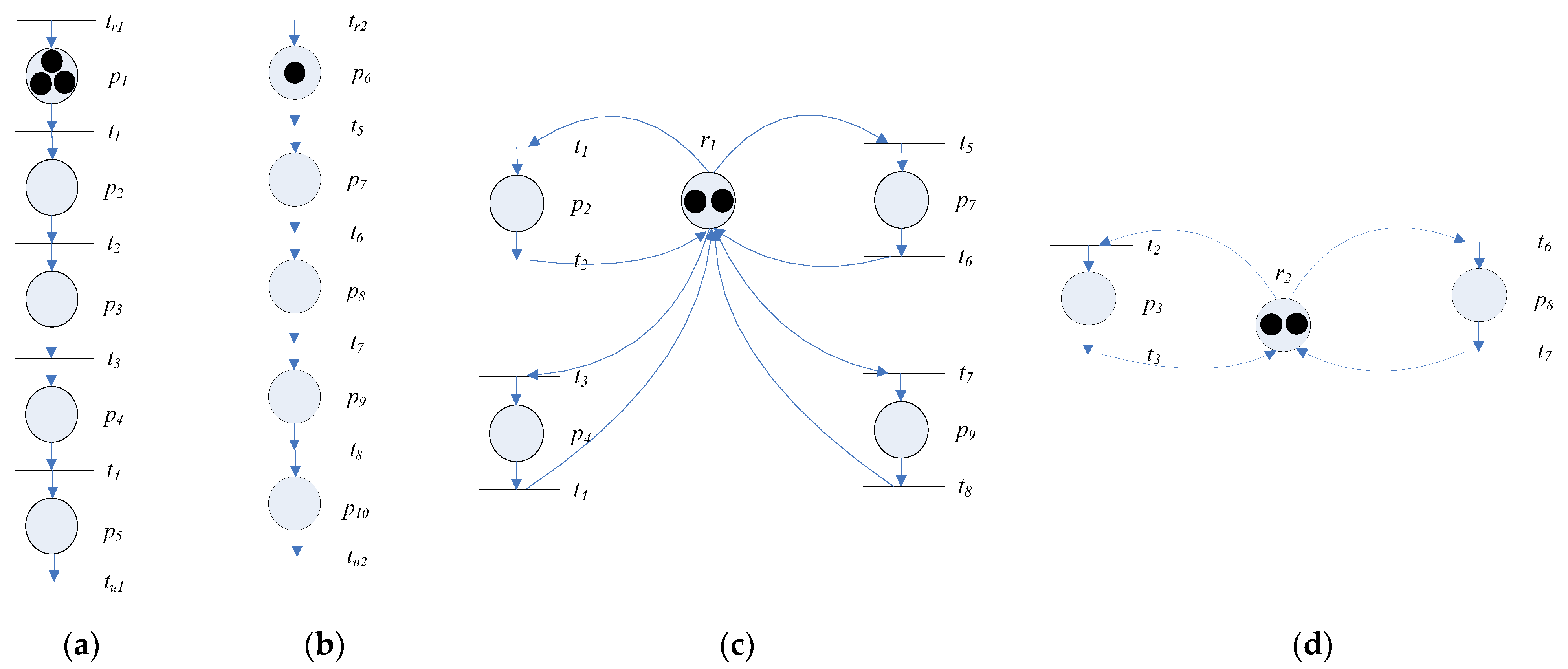
Two examples of the task subnets $G{J}_1$ and $G{J}_2$ can be found in Figure 1a,b.

Definition 2.

[Resource subnet]: A type-$r$ resource subnet,$r\in \mathit{R}$, is a discrete timed Petri net $G{R}_r=(P_r,T_r,F_r,m_{r0},{\mu }_r)$consisting of a number of activities represented by a circuit [17] of transitions and places, where $P_r$ is the set of all places in the circuits;$T_r$ is the set of transitions in the circuits;$F_r$ is the flow relation; $m_{r0}$ is the initial marking; ${\mu }_r:T_r\to Z$ specifies the firing time of each transition in $T_r$. The idle state of $G{R}_r$ is denoted by $r$.

Two examples of resource subnets $G{R}_1$ and $G{R}_2$ can be found in Figure 1c,d. $G{R}_1$ consisted of four circuits, $r_1{t}_1{p}_2{t}_2$, $r_1{t}_3{p}_4{t}_4$, $r_1{t}_5{p}_7{t}_6$ and $r_1{t}_7{p}_9{t}_8$. $G{R}_2$ consisted of two circuits, $r_2{t}_2{p}_3{t}_3$ and $r_2{t}_6{p}_8{t}_7$.

To take into account the interactions between each task subnet, $G{J}_j$ and $j\in \mathit{J}$, and each resource subnet, $G{R}_r$ and $r\in \mathit{R}$, we adopted the composition operator $“\Vert ”$, defined in [16]. The composition operator $“\Vert ”$ was applied to a set of discrete timed Petri nets to represent the synchronization of resources and workflows. The definition of the composition operator $“\Vert ”$ is as follows:

Definition 3.

[Composition operator] [19]: Given two discrete timed PNs, $G_1=(P_1,T_1,F_1,m_{10},{\mu }_1)$ and $G_2=(P_2,T_2,F_2,m_{20},{\mu }_2)$, the operator $“\Vert ”$ is used to combine $G_1$ and $G_2$ and is defined as follows:

$$\begin{gathered} G_1\Vert G_2=(P,T,F,m,\mu ), \mathrm{where} P=P_1\cup P_2, T=T_1\cup T_2 \\ \begin{array}{c}F(p,t)=\{\begin{array}{l}{F}_1(p,t)\hspace{0.17em}if\hspace{0.17em}p\in P_1\hspace{0.17em}and\hspace{0.17em}t\in T_1\\ F_2(p,t)\hspace{0.17em}if\hspace{0.17em}\in P_2\hspace{0.17em}and\hspace{0.17em}t\in T_2\end{array}, F(t,p)=\{\begin{array}{l}{F}_1(t,p)\hspace{0.17em}if\hspace{0.17em}p\in P_1\hspace{0.17em}and\hspace{0.17em}t\in T_1\\ F_2(t,p)\hspace{0.17em}if\hspace{0.17em}\in P_2\hspace{0.17em}and\hspace{0.17em}t\in T_2\end{array},\\ m_0(p)=\{\begin{array}{l}{m}_{10}(p)\hspace{0.17em}if\hspace{0.17em}p\in P_1\\ m_{20}(p)\hspace{0.17em}if\hspace{0.17em}p\in P_2\end{array}\mathrm{and}\mu (t)=\{\begin{array}{l}\max ({\mu }_1(t),{\mu }_2(t))\hspace{0.17em}if\hspace{0.17em}t\in T_1\cap \hspace{0.17em}{T}_2\\ {\mu }_1(t),\hspace{0.17em}if\hspace{0.17em}t\in T_1\backslash T_2\\ {\mu }_2(t),\hspace{0.17em}if\hspace{0.17em}t\in T_2\backslash T_1\hspace{0.17em}\end{array}\end{array} \end{gathered}$$

Definition 4.

[Nominal cyber world model of CPPS]: The nominal cyber world model of CPPS is a discrete timed Petri net$G=(P,T,F,m_0,\mu )=GJ\Vert GR$with$GJ=\underset{j\in \mathit{J}}{\Vert }G{J}_j$and$GR$ = $\underset{r\in \mathit{R}}{\Vert }G{R}_r$, obtained by merging all the task subnets and resource subnets in the system, where $m_0:P\to Z^{\left|P\right|}$. A state of $G$ is a vector $m\in Z^{\left|P\right|}$ referred to as a marking.

The model of CPPS obtained by $G=(P,T,F,m_0,\mu )=G{J}_1\Vert G{J}_2\Vert G{R}_1\Vert G{R}_2$ is depicted in Figure 2; $G{J}_1$, $G{J}_2$, $G{R}_1$ and $G{R}_2$ are defined in Figure 1.

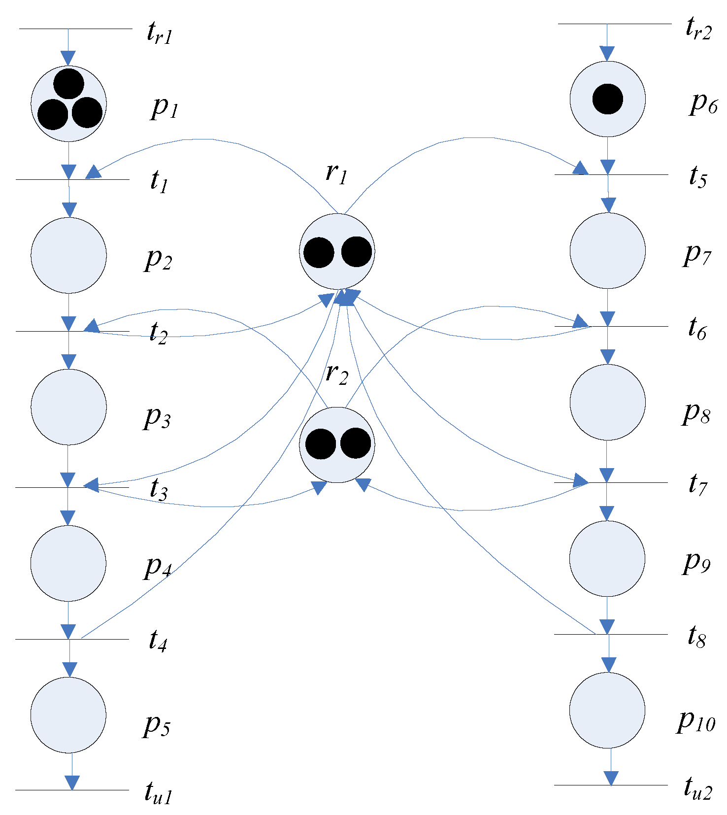
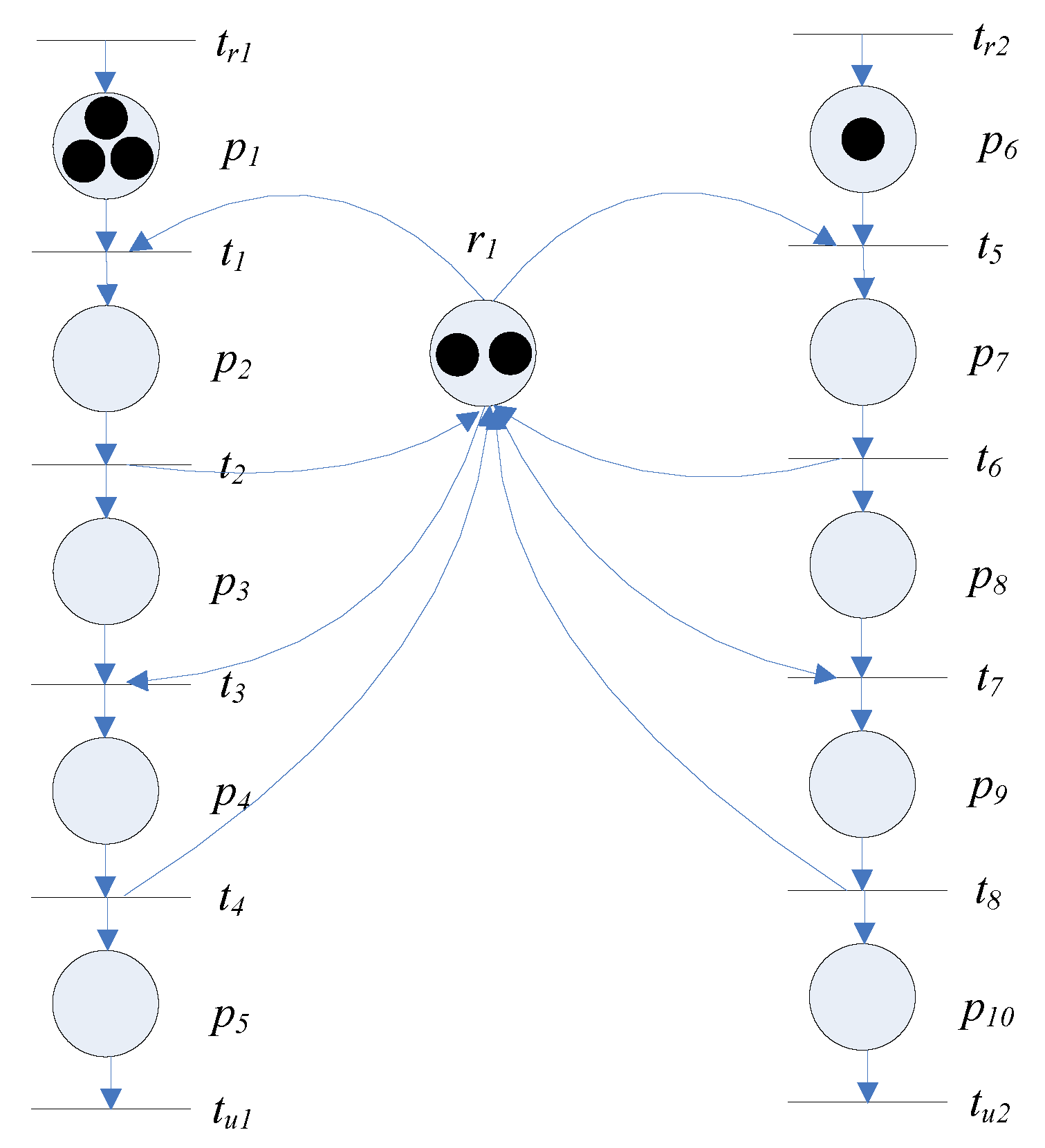
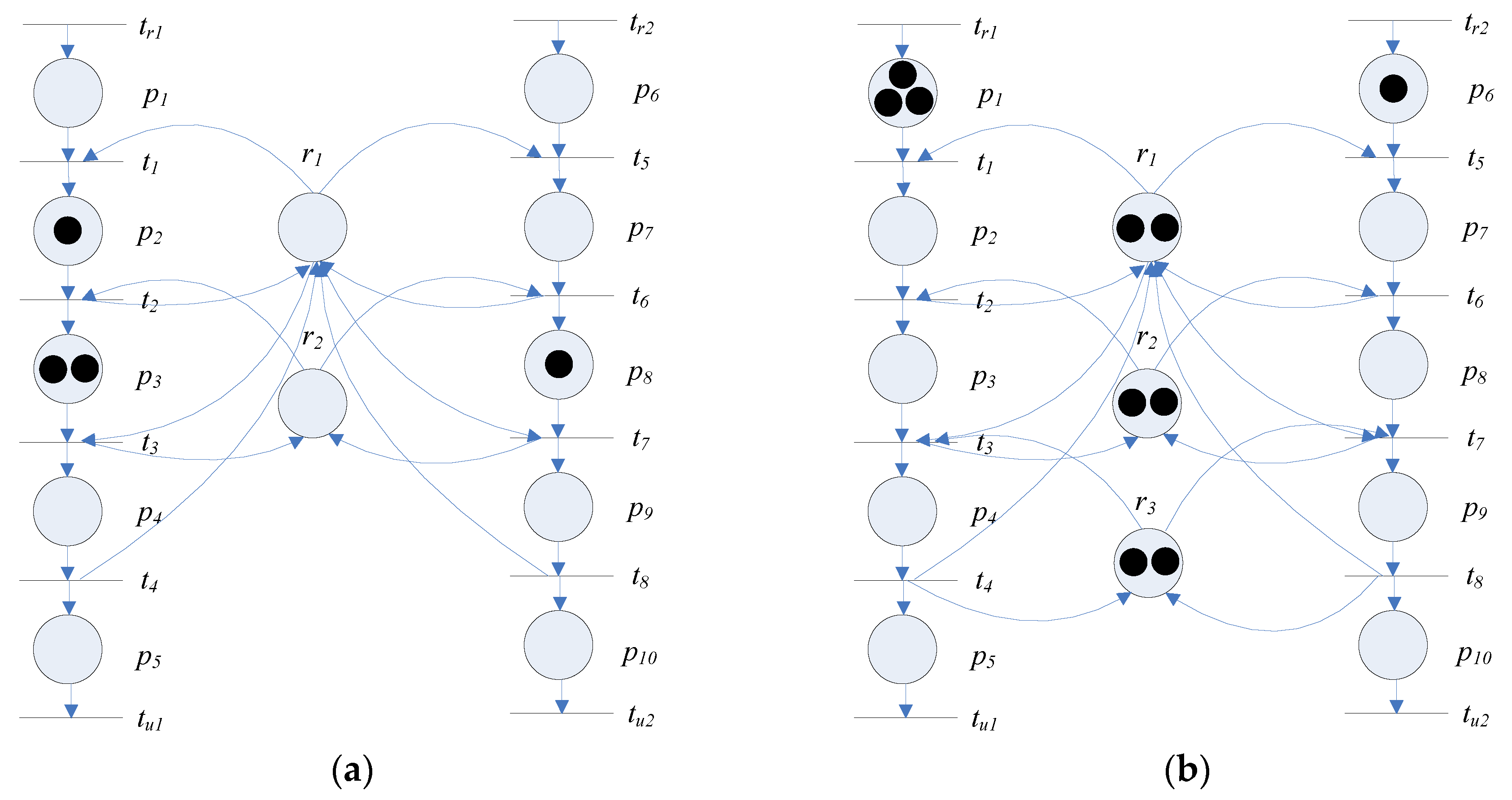
We illustrate the differences between the CPPS models used in this study and the one proposed in [18] by an example. Figure 3 shows an example of the class of models proposed in [18] extended with start and end transitions. For each transition in the model of Figure 3, there was at most one resource required for firing the transition and there was no “hold-and-wait” situation. However, a “hold-and-wait” situation might be required for firing a transition in the manufacturing systems. The CPPS models proposed in this study allowed modelling the “hold-and-wait” situation for firing a transition. For example, resources $r_2$ and $r_2$ were required to fire transitions $t_2$, $t_3$, $t_6$ and $t_7$ in Figure 2. Without a proper control policy, multiple resource requirements for firing a transition might lead to an undesirable state. Figure 4a shows the situation after executing the firing sequence $t_5{t}_6{t}_1{t}_2{t}_1{t}_2{t}_1$ to reach an undesirable state in which no transition could be fired any longer. Therefore, a proper control method must be used to prevent the system from visiting undesirable states.

The nominal cyber world model of CPPS $G=(P,T,F,m_0,\mu )$ proposed in this study allowed modeling operations requiring multiple resources. That is, firing a transition that required the allocation of multiple resources can be captured and represented in the proposed nominal cyber world model of CPPS $G=(P,T,F,m_0,\mu )$. The method proposed in this study could be applied to the nominal cyber world model of CPPS $G=(P,T,F,m_0,\mu )$ in which any transition in $T$ might require the allocation of multiple resources. Figure 4b shows an example of a nominal cyber world model of CPPS $G=(P,T,F,m_0,\mu )$ in which firing transitions $t_3$ and $t_7$ required the allocation of multiple resources, including one type-1 and one type-3 resource.

3.2. Robustness Problem and Resilience Problem

The nominal cyber world model of CPPS $G=(P,T,F,m_0,\mu )$ might evolve from the initial state $m_0$ through firing transitions and bring $G$ to a new state in different ways. However, firing transitions arbitrarily will not bring $G$ to a target state and may bring $G$ to an undesirable state, which cripples the CPPS. To direct the CPPS to the target state, a proper control policy must be applied. A control policy is specified by a sequence of control actions to guide the behaviors of $G$ to reach a target state while preventing the system from visiting undesirable states by controlling the firing of transitions under each state reached from the initial state. More formally, a control action is defined as follows:

Definition 5.

[Control action]: Given a CPPS model$G=(P,T,F,m_0,\mu )$, a transition is called a controlled transition if the number of times for firing the transition can be controlled by an external controller. The set of controlled transitions in $G=(P,T,F,m_0,\mu )$is denoted as$T_c$, where$T_c\subseteq T$. A control action $c$of$G=(P,T,F,m_0,\mu )$specifies the number of times each transition in$T_c$must be concurrently fired and is represented by a vector in $Z^{\left|T_c\right|}$.

Definition 6.

[Control policy]: Given a CPPS model $G=(P,T,F,m_0,\mu )$, a control policy $u$is defined as a sequence of control actions {$c_n$} of$G=(P,T,F,m_0,\mu )$. That is,$u$:$R(m_0)\to Z^{\left|T_c\right|}$. The CPPS model$G=(P,T,F,m_0,\mu )$operating under a control policy$u$is denoted by$G_c=(P,T,F,m_0,\mu ,u)$. We refer to $G_c=(P,T,F,m_0,\mu ,u)$as$G_c=(m_0,u)$for brevity.

To ensure that $G_c=(P,T,F,m_0,\mu ,u)$ does not visit any undesirable states, the liveness concept was introduced for a control policy, as follows:

Definition 7.

[Liveness]:$G_c=(m_0,u)$is live if, for each marking reached from$m_0$under$u$, each transition can still ultimately be fired by progressing through some further firing sequence.

The objective of CPPS is to meet the order demand by a deadline $\mathrm{\Phi }$ without visiting any undesirable states. Suppose the order demand for type-$j$ tasks was $D_j$ and $j\in \mathit{J}$. This requirement could be stated by specifying a final marking $m_f$ for $G_c=(P,T,F,m_0,\mu ,u)$ to represent that the requested quantities of different types of tasks were completed and stayed in the corresponding final state places of task subnets, where $m_f(p)=\{\begin{array}{l}{m}_0(p)\hspace{0.17em}if\hspace{0.17em}p\in P_o\\ D_j\hspace{0.17em}if\hspace{0.17em}p\in P_F\\ 0\hspace{0.17em}if\hspace{0.17em}p\in P\backslash (P_o\cup P_F)\end{array}$. $P_o$ is the set of idle state places of all resource subnets and $P_F=\{p_{jn}|j\in \mathit{J}\}$ is the set of final state places of all types of task subnets. So the problem to meet the order requirements was to determine a control policy $u$ for $G_c=(P,T,F,m_0,\mu ,u)$ such that final marking $m_f$ could be reached from $m_0$ by the deadline $\mathrm{\Phi }$ without visiting any undesirable states. A control policy $u$, under which $G_c=(m_0,u)$ was live, ensured that no undesirable state was visited.

In the previous study [19], the connection between the existence of a live control policy and an optimization problem called nominal optimization problem (NOP) formulated based on the joint spatial-temporal network (JSTN) was established, where Procedure 1 in Appendix B was used to construct the joint spatial-temporal network $JSTN(V,A)$ of $G_c=(P,T,F,m_0,\mu ,u)$. The nominal optimization problem is defined in Expressions (1) through (6) as follows:

Nominal optimization problem (NOP) based on the joint spatial-temporal network

$$\underset{f}{\min }\sum _{a(v,w)\in A}\lambda (a(v,w))f(a(v,w))$$

(1)

$$\sum _{j\in \mathit{J}}\sum _{a(v,w)\in A_{jr\tau }}f(a(v,w))\le C_{r\tau }\forall r\in \mathit{R}\hspace{0.17em}\forall \tau \in \{1,2,\dots ,\mathrm{\Pi }\}$$

(2)

$$\sum _{w\in V(v)}f(a(v,w))=0\hspace{0.17em}\forall v\in V\backslash \{s\}\backslash \{e_j\forall j\in \mathit{J}\}$$

(3)

$$\sum _{w\in V_j(s)}f(a(s,w))=D_j\hspace{0.17em}\hspace{0.17em}\forall j\in \mathit{J}$$

(4)

$$\sum _{w\in V_j(e_j)}f(a(w,e_j))=D_j\hspace{0.17em}\hspace{0.17em}\forall j\in \mathit{J}\hspace{0.17em}$$

(5)

$$f(a(v,w))\in \mathrm{Z}\hspace{0.17em}\forall a(v,w)\in A,\mathrm{where}\mathrm{Z}\mathrm{is}\mathrm{the}\mathrm{set}\mathrm{of}\mathrm{nonnegative}\mathrm{integers}$$

(6)

The problem of determining the existence of a control policy to keep $G_c=(m_0,u)$ live while reaching final state $m_f$ was checked according to the following theorem [16]:

Theorem 1

([19]).There exists a solution to the nominal optimization problem if and only if there exists a control policy under which$G_c=(m_0,u)$is live and can reach$m_f$under$u$.

If multiple control policies exist, there exists multiple solutions. Surely, in case of multiple control policies existing, there was at least one solution. If there were multiple solutions, there existed multiple control policies. Theorem 1 also holds for the case of multiple control policies or a multiple solutions situation.

In CPPS, the goal of fulfilling order requirements requires two sub-goals to be attained: to produce the products to meet the product demand and to meet the order due date. The occurrence of resource failures has negative impacts on CPPS. If the impacts are not great enough, and the product demand as well as the due date can still be meet after recovering from resource failures, the CPPS is said to be robust with respect to resource failures. If the impacts of resource failures are so great that the due date can no longer be met even if the product demand can be met, the CPPS is said to be resilient with respect to resource failures. Note that in our definition, if CPPS is robust with respect to given resource failures, the goal can still be achieved. If CPPS is not robust with respect to resource failures, but the CPPS is resilient with respect to the resource failures, the product demand can be produced, but the due date cannot be met. In short, we use the terms “robust” and “resilient” to distinguish whether the original goal can be completely or partially achieved. If both the sub-goal of producing the products to meet the product demand and the sub-goal of meeting the order due date can be achieved in the presence of the failures, the CPPS is robust with respect to given resource failures. If only the sub-goal to produce the products to meet the product demand can be achieved, the CPPS is resilient with respect to the resource failures.

In this study, we focused on the resilience and robustness properties of CPPS with respect to uncertainties due to resource failures. Resilience property of CPPS refers to the ability to achieve the objective to reach the goal state $m_f$ in the presence of uncertainties without visiting undesirable states. Robustness property of CPPS is concerned with the capability to achieve the objective to reach the goal state $m_f$ by the deadline in the presence of uncertainties without visiting undesirable states. To develop a solution method, a model of uncertainties must be introduced for the model $G$ of CPPS. In CPPS, uncertainties due to resource failures are reflected in the unavailability of resources. Resource failures in CPPS typically lead to changes in the number of available resources. In terms of the model $G$ of CPPS, changes in the number of available resources can be represented by perturbation in the marking of the model $G$. Although the perturbation in the marking of the model $G$ can describe the number of resources that are unavailable due to failures, it does not describe how long the failures last or the duration of the failures. For this reason, we introduced the failure time interval vector to describe the duration of resource failures in CPPS. Based on the discussions above, we introduced the following model of uncertainties.

Definition  8.

[Model of uncertainties]: Given a marking$m$of the model$G$of CPPS, a model of uncertainties is represented by a perturbation vector$\delta$= [${\delta }_{p_1}$,${\delta }_{p_2}$,…,${\delta }_{p_{\left|P\right|}}$] of$m$with${\delta }_p$denoting the perturbation due to failures at place$\forall p\in P$and a failure time interval vector$\omega$defined by the element${\omega }_{pl}$=$[{\alpha }_{pl}\hspace{0.17em}{\beta }_{pl}]$, the interval of periods for a failure at the place$p$, where$p\in P$and$l\in \{1,2,\dots ,{\delta }_p\}$. The model ofuncertainties is represented by$\Delta (m)$= ($m$,$\delta$,$\omega$). Note that${\delta }_p\le m(p)\forall p\in P$.

With the model of uncertainties defined above, we defined the resilience problem and the robustness problem in CPPS as follows.

The resilience problem in CPPS can be stated as the problem of determining whether there exists a control policy to bring $G$ to the marking $m_f$ without visiting any undesirable states under $\Delta (m)$ = ($m,\delta$,$\omega$), where $m_f$ and the deadline $\mathrm{\Phi }$ are the final marking and the deadline corresponding to the given order requirements, respectively.

The robustness problem in CPPS can be stated as the problem of determining whether there exists a control policy to bring $G$ to the marking $m_f$ by the deadline $\mathrm{\Phi }$ without visiting any undesirable states under $\Delta (m)$ = ($m$,$\delta$,$\omega$), where $m_f$ and the deadline $\mathrm{\Phi }$ are the final marking and the deadline corresponding to the given order requirements, respectively.

Motivated by the two problems stated above, we defined the resilience and robustness properties of CPPS as follows:

Definition 9.

[Resilience with respect to uncertainties]: A CPPS is resilient with respect to$\Delta (m)$if there exists a control policy$u$under which$G_c=(m_0,u)$can reach$m_f$in the presence of$\Delta (m)$.

Definition 10.

[Robustness with respect to uncertainties]: A CPPS is robust with respect to$\Delta (m)$if there exists a control policy$u$under which$G_c=(m_0,u)$can reach$m_f$by the deadline$\mathrm{\Phi }$in the presence of$\Delta (m)$.

The resilience problem and robustness problem in CPPS stated above are analyzed in the next section.

4. Robustness Analysis Method for a Class of CPPS

In this section, the analysis of the resilience and robustness problems in CPPS was completed. We first presented the loss of capacity due to $\Delta (m)$ and then formulated a problem to find the solution to accommodate the changes in resource capacity due to $\Delta (m)$.

The occurrence of $\Delta (m)$ = ($m,\delta$,$\omega$) changed the capacity of resources in CPPS. We represented the capacity of resources under $\Delta (m)$ as follows:

Definition 11.

[Capacity of a resource under$\Delta (m)$]: Given a marking$m$of the model$G$of CPPS, the capacity of type-$r$resources in period$\tau$under perturbation$\Delta (m)$= ($m$,$\delta$,$\omega$) is represented by$C_{r\tau }^{\Delta (m)}$.

As the capacity of resources was changed due to the failures of resources under $\Delta (m)$ = ($m$,$\delta$,$\omega$), the problem of determining the existence of a control policy to maintain the liveness of $G_c$ should take into account the changes in resource capacity due to $\Delta (m)$.

To compute the change of capacity under $\Delta (m)$, we needed the following definitions.

Definition 12.

[Relation between a place and different types of resources]: The relation between a place$p\in P$and the different types of resources is represented by${\mathrm{\Gamma }}_{pr}=\{\begin{array}{l}1\hspace{1em}if\hspace{1em}p\in P\cap (P_r\backslash \{r\})\hspace{1em}\\ 0\hspace{1em}otherwise\end{array}$.

Definition 13

[Influence of failure at a place on capacity of resources in a period]: We used${\mathrm{\Omega }}_{pl\tau }$to denote whether the $l$-th failure at place$p$influenced the capacity of the corresponding resources in period$\tau$, where${\mathrm{\Omega }}_{pl\tau }=\{\begin{array}{l}1\hspace{1em}if\hspace{1em}\tau \in [{\alpha }_{pl}\hspace{0.17em}{\beta }_{pl}]\hspace{1em}\\ 0\hspace{1em}otherwise\end{array}$.

Lemma 1.

Given a marking$m$of the model$G$of CPPS and uncertainties model$\Delta (m)$= ($m$,$\delta$,$\omega$), the reduction of type-$r$resource capacity in period$\tau$due to$\Delta (m)$is${\displaystyle \sum _{p\in P}}{\mathrm{\Gamma }}_{pr}({\displaystyle \sum _{l=1}^{{\delta }_p}{\mathrm{\Omega }}_{pl\tau })}$.

Proof.

A failure at place $p$ may influence the type-$r$ resources only if. The $l$-th failure at place $p$ may influence the capacity of some types of resources in period $\tau$ only if ${\mathrm{\Omega }}_{pl\tau }=1$. Therefore, the $l$-th failure at place $p$ may reduce the capacity of type-$r$ resources in period $\tau$ by one only if ${\mathrm{\Gamma }}_{pr}{\mathrm{\Omega }}_{pl\tau }=1$.

Therefore, the reduction of the number of type-$r$ resources in period $\tau$ due to all failures at place $p$ under $\Delta (m)$ is ${\mathrm{\Gamma }}_{pr}({\displaystyle \sum _{l=1}^{{\delta }_p}{\mathrm{\Omega }}_{pl\tau })}$.

By taking into account the failures at all places, the reduction of the number of type-$r$ resources in period $\tau$ due to all failures at place $p$ under $\Delta (m)$ is ${\displaystyle \sum _{p\in P}}{\mathrm{\Gamma }}_{pr}({\displaystyle \sum _{l=1}^{{\delta }_p}{\mathrm{\Omega }}_{pl\tau })}$.

This completes the proof. □

Let $C_{r\tau }^{\Delta (m)}$ denote the capacity of type-$r$ resources in period $\tau$ due to all failures $\Delta (m)$. As Lemma 1 holds for each type of resources, $C_{r\tau }^{\Delta (m)}$ = $C_{r\tau }-{\displaystyle \sum _{p\in P}}{\mathrm{\Gamma }}_{pr}({\displaystyle \sum _{l=1}^{{\delta }_p}{\mathrm{\Omega }}_{pl\tau })}$$\forall r\in \mathit{R}$. The residual capacity under $\Delta (m)$ is ${\tilde{C}}_{rt}=C_{r\tau }^{\Delta (m)}-{\displaystyle \sum _{j\in \mathit{J}}}{\displaystyle \sum _{a=(v,w)\in A_{jrt}}}{f}_u(v,w)$, which is equal to Expression (7):

$${\tilde{C}}_{rt}=C_{r\tau }-{\displaystyle \sum _{p\in P}}{\mathrm{\Gamma }}_{pr}({\displaystyle \sum _{l=1}^{{\delta }_p}{\mathrm{\Omega }}_{pl\tau })}-\sum _{j\in \mathit{J}}\sum _{a=(v,w)\in A_{jrt}}{f}_u(v,w)\hspace{0.17em}r\in \mathit{R}\hspace{0.17em}\forall t\in \{1,2,\dots ,\mathrm{\Pi }\}$$

(7)

Definition 14.

[Residual Capacity]: The residual capacity under$\Delta (m)$is${\tilde{C}}_{rt}=C_{r\tau }-{\displaystyle \sum _{p\in P}}{\mathrm{\Gamma }}_{pr}({\displaystyle \sum _{l=1}^{{\delta }_p}{\mathrm{\Omega }}_{pl\tau })}-{\displaystyle \sum _{j\in \mathit{J}}}{\displaystyle \sum _{a=(v,w)\in A_{jrt}}}{f}_u(v,w)\hspace{0.17em}r\in \mathit{R}\hspace{0.17em}\forall t\in \{1,2,\dots ,\mathrm{\Pi }\}$.

In this study, a new method was developed to analyze the resilience and robustness properties of CPPS. We formulated an alternative solution optimization problem (ASOP) to find an alternative solution based on the nominal solution and tested the resilience and robustness properties of the perturbed system. Let $f$ denote the nominal solution of NOP. A nominal solution $f$ can be divided into two or more components called sub-solutions in this study. We divided the nominal solution $f$ into the sub-solution $f_u$ not influenced by $\Delta (m)$ and the sub-solution $f_{\Delta }$ influenced by $\Delta (m)$ with $f=f_u+f_{\Delta }$.

The flow $f_{\Delta }$ influenced by the resource failures associated with perturbation $\Delta (m)$ = ($m$,$\delta$,$\omega$) can be divided into two parts. That is, the flow ${}^{~}f{}_{\Delta }$ at upstream of the failed places (including the places in which the failures occurred) and the flow $f_{\Delta }^{~}$ at downstream of the failed places. For the flow of ${}^{~}f{}_{\Delta }$, all the relevant operations have been executed. All the used capacities of resources involved with ${}^{~}f{}_{\Delta }$ cannot be changed. For the flow at the downstream of the failed place, $f_{\Delta }^{~}$, capacity of the resources not failed can still be used for performing operations. Based on the discussion above, we can calculate the residual capacity for $JSTN(V,A)$ by applying Procedure 2 from

Table A3. Procedure 2 to calculate residual capacity.

Procedure 2: Calculation of Residual Capacity ${\tilde{C}}_{rt}$$\forall r\in \mathit{R}$, $t\in \{1,2,\dots ,\mathrm{\Pi }\}$,$f_u$,$f_{\Delta }$ and $\Delta D_j$$\forall j\in \mathit{J}$
Input: $JSTN(V,A)$,$f$,$\theta$,$\delta$,$\Delta (m)$ = ($m$,$\delta$,$\omega$),$C_{rt}$,$\forall r\in \mathit{R}$,$t\in \{1,2,\dots ,\mathrm{\Pi }\}$
Output: ${\tilde{C}}_{rt}\forall r\in \mathit{R}$,$t\in \{1,2,\dots ,\mathrm{\Pi }\}$,$f_u$,$f_{\Delta }$ and $\Delta D_j$$j\in \mathit{J}$
Step 1: Find the flows $f_u$ in the nominal solution $f$ not influenced by resource failures             $\delta$             Find the flows $f_{\Delta }$, ${}^{~}f{}_{\Delta }$ and $f_{\Delta }^{~}$ according to the nominal solution $f$             influenced by resource failures $\Delta (m)$             Find $\Delta D_j$, the quantity of type-$j$ products in $f_{\Delta }$ influenced by resource             failures $\Delta (m)$ for each $j\in \mathit{J}$:             For $j\in \mathit{J}$                   If $j$ is equal to 1                      $k\leftarrow 0$                   Else                         $k\leftarrow {\displaystyle \sum _{j=1}^{j-1}}(N_{j^{\prime }}+1)(\mathrm{\Pi }+1)$                   End If                   $\Delta D_j\leftarrow {}_{}{}^{~}f{}_{\Delta }(s_j,k+(n-1)(\mathrm{\Pi }+1)+1)$             End For Step 2: ${\tilde{C}}_{rt}\leftarrow C_{rt}$for each $r\in \mathit{R}$ for each period $t\in \{1,2,\dots ,\mathrm{\Pi }\}$             Update the residual resource capacity ${\tilde{C}}_{rt}$ for each $r\in \mathit{R}$ for each period$t$:             Removing the resource capacities originally allocated to $f_u$ from ${\tilde{C}}_{rt}$ for $r\in \mathit{R}$,             $j\in \mathit{J}$             Removing the resource capacities due to resource failures $\delta$ in $\Delta (m)$ from ${\tilde{C}}_{rt}$:             ${\tilde{C}}_{rt}=C_{rt}-{\displaystyle \sum _{j\in \mathit{J}}}{\displaystyle \sum _{a=(v,w)\in A_{jrt}}}{f}_u(v,w)-C_{rt}^{\delta }\forall r\in \mathit{R}\hspace{0.17em}\forall t\in \{1,2,\dots ,\mathrm{\Pi }\}$, where $C_{rt}^{\delta }$ is the             capacity loss due to type-$r$ resource failures $\delta$ under $\Delta (m)$.

of Appendix B, where we also calculated the quantity $\Delta D_j$ of type-$j$ products influenced by $\Delta (m)$ for each $j\in \mathit{J}$. For a given nominal solution $f$, we calculate the residual capacity ${\tilde{C}}_{rt}$ of type-$r$ resources for each period $t$ by deducting the capacity used by $f_u$ and ${}^{~}f{}_{\Delta }$ and the capacity loss in the failed places due to perturbation $\Delta (m)$. In finding an alternative solution for the influenced flows, an objective function should be defined, and three types of constraints must be satisfied: (a) capacity constraints, (b) flow balance constraints and (c) flow constraints due to influenced flow ${}^{~}f{}_{\Delta }$. The objective function defined in Expression (8) was used to minimize the overdue penalty. The capacity constraints are described by Expression (9) enforce that allocated operations must be no greater than the residual capacity ${\tilde{C}}_{rt}=C_{r\tau }-{\displaystyle \sum _{p\in P}}{\mathrm{\Gamma }}_{pr}({\displaystyle \sum _{l=1}^{{\delta }_p}{\mathrm{\Omega }}_{pl\tau })}-{\displaystyle \sum _{j\in \mathit{J}}}{\displaystyle \sum _{a=(v,w)\in A_{jrt}}}{f}_u(v,w)$ for $r\in \mathit{R}$ and $t\in \{1,2,\dots ,\mathrm{\Pi }\}$ under $\Delta (m)$.

The flow balance constraints for the influenced flow are described in Expressions (10)–(12). The flow constraints due to influenced flow ${}^{~}f{}_{\Delta }$ are described in Expression (13), which indicated that the flow value of each arc in the path of ${}^{~}f{}_{\Delta }$ in the alternative solution must be the same as the flow value in the corresponding arc of ${}^{~}f{}_{\Delta }$. The constraint in Expression (14) states that the decision variables must be nonnegative integers.

We formulated an alternative solution optimization problem (ASOP) to find an alternative solution to accommodate the changes in resource capacity due to $\Delta (m)$.

Alternative solution optimization problem (ASOP)

$$\underset{f}{\min }\sum _{a(v,w)\in A}\lambda (a(v,w))f(a(v,w))$$

(8)

$$\sum _{j\in \mathit{J}}\sum _{a(v,w)\in A_{jr\tau }}f(a(v,w))\le {\tilde{C}}_{rt}\forall r\in \mathit{R}\hspace{0.17em}\forall \tau \in \prod =\{1,2,\dots ,\mathrm{\Pi }\}$$

(9)

$$\sum _{w\in V(v)}f(v,w)=0\hspace{0.17em}\forall v\in V\backslash \{s\}\backslash \{e_j\forall j\in \mathit{J}\}$$

(10)

$$\sum _{w\in V_j(s)}f(s,w)=\Delta D_j\hspace{0.17em}\hspace{0.17em}\forall j\in \mathit{J}$$

(11)

$$\sum _{w\in V_j(e_j)}f(w,e_j)=\Delta D_j\hspace{0.17em}\hspace{0.17em}\forall j\in \mathit{J}\hspace{0.17em}$$

(12)

$${}^{~}f{}_{\Delta }(v,w)(f(v,w)-{}^{~}f{}_{\Delta }(v,w))=0\forall (v,w)\in A$$

(13)

$$f(a(v,w))\in \mathrm{Z}\hspace{0.17em}\forall a(v,w)\in A,\mathrm{where}\mathrm{Z}\mathrm{is}\mathrm{the}\mathrm{set}\mathrm{of}\mathrm{nonnegative}\mathrm{integers}.$$

(14)

Assumption 1:

In this study, we assumed that the function$g(\tau )$used by Function 1 in Appendix B satisfied $g(\tau )$= 0 for$\tau \le \mathrm{\Phi }$. Under this setting, there was no penalty if the requested tasks were completed by the deadline$\mathrm{\Phi }$. We also assumed that the function$h(\tau )$used by Function 1 in Appendix B satisfied$h(\tau )>0$for$\tau >\mathrm{\Phi }$. Under this setting, there was penalty if the requested tasks were completed by the deadline$\mathrm{\Phi }$.

Under the setting of Assumption 1, Theorem 2 provides the conditions to check the resilience and robustness properties of CPPS.

Theorem 2.

Suppose Assumption 1 holds. Let$f$denote the nominal solution of NOP and$f$is divided into the sub-solution$f_u$not influenced by$\Delta (m)$and the sub-solution$f_{\Delta }$influenced by$\Delta (m)$with$f=f_u+f_{\Delta }$. If there exists a solution$f_{\Delta }^{\prime }$for the ASOP, there exists a control policy$u$under which$G_c(m_0,u)$can reach$m_f$in the presence of$\Delta (m)$. In this case,$G_c(m_0,u)$is resilient with respect to$\Delta (m)$. If the objective function value of the solution$f$is zero and the objective function value of the solution$f_{\Delta }^{\prime }$for the ASOP is zero, there exists a control policy$u$under which$G_c(m_0,u)$can reach$m_f$by the deadline$\mathrm{\Phi }$in the presence of$\Delta (m)$. In this case,$G_c(m_0,u)$is robust with respect to$\Delta (m)$.

Proof. 

Please refer to Appendix A. □

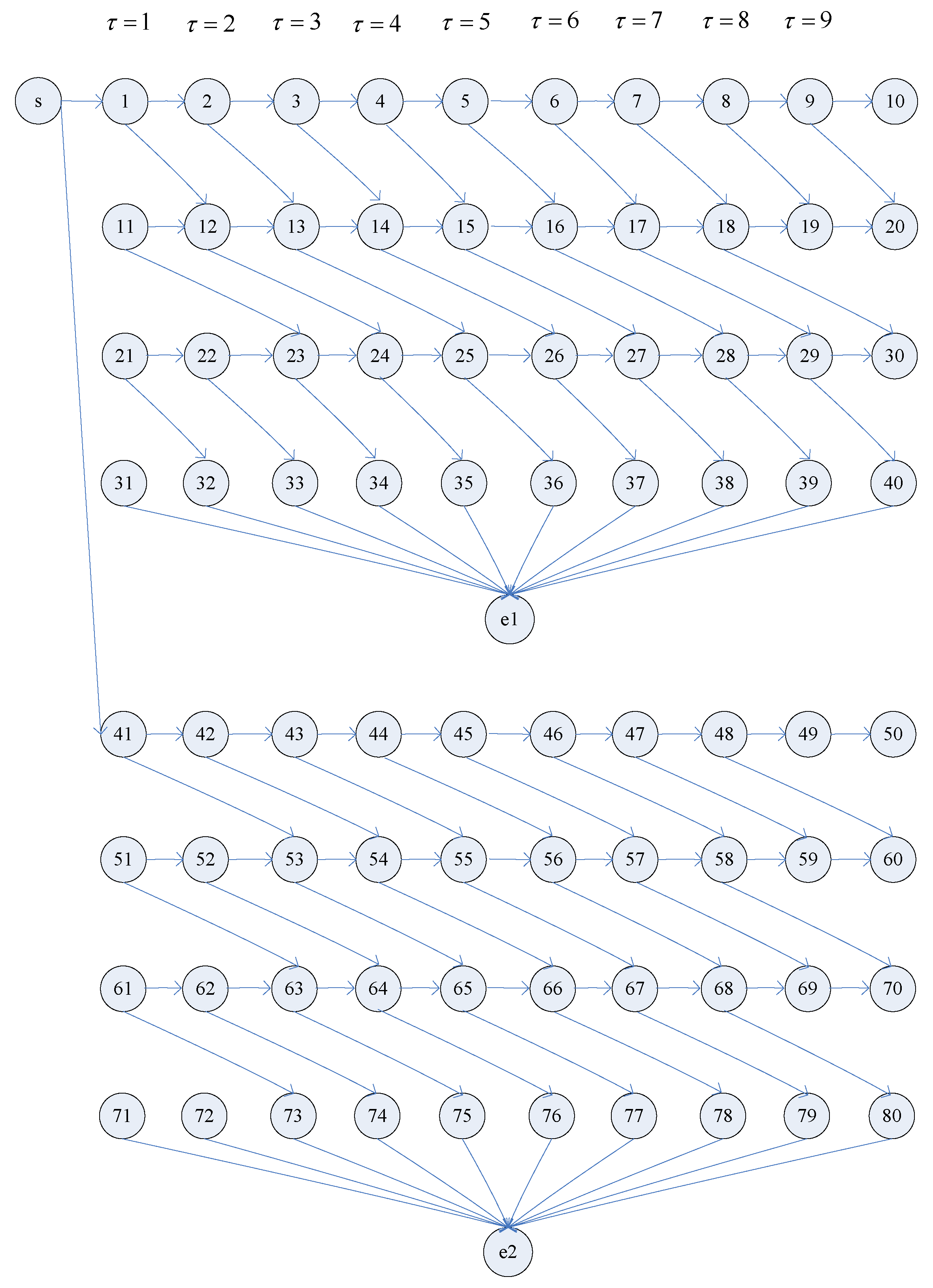
Note that the constraints in Expressions (9)–(12) and (14) of the ASOP resembled the constraints in Expressions (2)–(6) in NOP. Constraints in Expressions (10)–(12) of the ASOP could be represented by the joint spatial-temporal network $JSTN(V,A)$ of $G_c$. Therefore, a solution for the ASOP could be represented by the flows in the joint spatial-temporal network $JSTN(V,A)$, and the flows must satisfy the capacity constraint in Expression (9) and flow constraint in Expression (13). Figure 5 is an example of joint spatial-temporal network. Due to the network structure of constraints in Expressions (10)–(12), the ASOP is a class of linear network flow problem with additional constraints in Expressions (9) and (13). So ASOP is a minimal cost flow problem with additional constraints. Therefore, we developed a solution algorithm for handling uncertainty due to $\Delta (m)$ by constructing a joint spatial-temporal network $JSTN(V,A)$ of $G_c$, calculating residual capacity ${\tilde{C}}_{rt}$$\forall r\in \mathit{R}$, $t\in \{1,2,\dots ,\mathrm{\Pi }\}$, $f_u$, $f_{\Delta }$ and $\Delta D^{j}j\in \mathit{J}$ and finding the solution $f_{\Delta }^{\prime }$ for the ASOP defined by $JSTN(V,A)$ with residual capacity ${\tilde{C}}_{rt}$ and $\Delta D_j$$j\in \mathit{J}$.

Based on the above discussion and Theorem 2, we proposed Algorithm 1 to facilitate assessment of the impacts of resource failures by checking the resilience and robustness properties of CPPS.

Algorithm 1: Construction of an Alternative Solution for$\Delta (m)$

Input: The nominal solution $f$,$\theta$,$\delta$,$\Delta (m)$ = ($m$,$\delta$,$\omega$)

Output: Resilience_Indicator, Robust_Indicator, $f^{\prime }$,$f_{\Delta }^{\prime }$

Step 0: Set Resilience_Indicator = false

Set Robust_Indicator = false

Step 1: Construct $JSTN(V,A)$ by applying Procedure 1.

Step 2: Apply Procedure 2 to calculate residual capacity ${\tilde{C}}_{rt}$$\forall r\in \mathit{R}$,$t\in \{1,2,\dots ,\mathrm{\Pi }\}$,$f_u$, $f_{\Delta }$ and $\Delta D_j$$\forall j\in \mathit{J}$, where $f_u$ denotes the flows not influenced by $\Delta (m)$ whereas $f_{\Delta }$ denotes the flows influenced by $\Delta (m)$, $\Delta D_j$ and $j\in \mathit{J}$ are the quantities of different types of products influenced by $\Delta (m)$.

Step 3: Set the capacity constraints of the ASOP defined by $JSTN(V,A)$

according to the residual capacity ${\tilde{C}}_{rt}$

Find the solution $f_{\Delta }^{\prime }$ for the ASOP as defined by $JSTN(V,A)$ with residual

capacity constraint ${\tilde{C}}_{rt}$ and $\Delta D_j$$j\in J$

If there exists a solution $f_{\Delta }^{\prime }$ for the ASOP

Update $f^{\prime }=f_u+f_{\Delta }^{\prime }$

Update residual capacity ${\tilde{C}}_{rt}$ by deducting the capacity assigned to $f^{\prime }$

from ${\tilde{C}}_{rt}$: ${\tilde{C}}_{rt}\leftarrow$${\tilde{C}}_{rt}-{\displaystyle \sum _{(v,w)\in A_{jrt}}}{f}_{\Delta }^{\prime }(v,w)$

Set Resilience_Indicator = true

If the objective function value of the solution $f_{\Delta }^{\prime }$ of the ASOP is zero,

Set Robust_Indicator = true

Else

Set Robust_Indicator = false

End If

End If

The steps of Algorithm 1 are briefly described as follows. Step 1 of Algorithm 1 constructs the joint spatial-temporal network $JSTN(V,A)$ of $G_c$. The algorithm to construct the joint spatial-temporal network $JSTN(V,A)$ of $G_c$ is shown in Function 1 and Procedure 1 in

Table A1. Function 1 to construct the spatial-temporal network (STN) for type-$j$ task subnet.

Function 1: Construction of Type-$j$ Spatial-Temporal Network [Source: Algorithm 1 in [19]]
Input: $G{J}_j$,$\mathrm{\Pi }$,$\mathrm{\Phi }$,$g(t)$,$h(t)$,$\Delta (m)$ = (m,$\delta$,$\omega$) and $f$
Output: $ST{N}_j(V_j,A_j)$, where $V_j$ is the set of nodes and $A_j$ is the set of arcs.
Step 0: Create the start node $s_j$             Create the end node $e_j$             $V_j\leftarrow \{s_j,e_j\}$             If $j$ is equal to 1             $k\leftarrow 0$             Else             $k\leftarrow {\displaystyle \sum _{j^{\prime }=1}^{j-1}}(N_{j^{\prime }}+1)(\mathrm{\Pi }+1)$             End If Step 1: For $n=1$ to $N_j+1$                    For each $\tau =1$ to $\mathrm{\Pi }+1$                          Create a node with number $k+(n-1)(\mathrm{\Pi }+1)+\tau$                          $V_j=V_j\cup \{k+(n-1)(\mathrm{\Pi }+1)+\tau \}$             End For          End For Step 2: Create arc $a(s_j,k+(n-1)(\mathrm{\Pi }+1)+\tau ))$ from node $s_j$ to node $k+(n-1)(\mathrm{\Pi }+1)+\tau$            $A_j\leftarrow A_j\cup \{a(s_j,k+(n-1)(\mathrm{\Pi }+1)+\tau ))\}$            Set arc cost $\lambda (a(s_j,k+(n-1)(\mathrm{\Pi }+1)+\tau )))\leftarrow 0$ Step 3: For $n=1$ to $N_j$                    For each $\tau =1$ to $\mathrm{\Pi }$                          Create an arc $a(k+(n-1)(\mathrm{\Pi }+1)+\tau ,k+(n-1)(\mathrm{\Pi }+1)+\tau +1))$                    $A_j\leftarrow A_j\cup \{a\}$                    Set arc cost $\lambda (a(k+(n-1)(\mathrm{\Pi }+1)+\tau ,k+(n-1)(\mathrm{\Pi }+1)+\tau +1))$ to 0                 End For              End For Step 4: For $n=1$ to $N_j$                    For each $\tau =1$ to $\mathrm{\Pi }$                      If $\tau +\mu (t_n)\le \mathrm{\Pi }+1$                                   Create arc                                   $a(k+(n-1)(\mathrm{\Pi }+1)+\tau ,k+n(\mathrm{\Pi }+1)+\tau +\mu (t_n))$                                   $A_j\leftarrow A_j\cup \{a(k+(n-1)(\mathrm{\Pi }+1)+\tau ,k+n(\mathrm{\Pi }+1)+\tau +\mu (t_n))\}$                                   Set arc cost $\lambda (a(k+(n-1)(\mathrm{\Pi }+1)+\tau ,k+n(\mathrm{\Pi }+1)+\tau +\mu (t_n)))\leftarrow 0$                                        If ${}^{•}t{}_n=\{r\}$                                                 $A_{jr\tau }\leftarrow A_{jr\tau }\cup \{a(k+(n-1)(\mathrm{\Pi }+1)+\tau ,k+n(\mathrm{\Pi }+1)+\tau +\mu (t_n))\}$                      End If                  End For              End For Step 5: For each $\tau =1$ to$\mathrm{\Pi }+1$                      Create arc $a(k+N_j(\mathrm{\Pi }+1)+\tau ,e_j)$ from node $k+N_j(\mathrm{\Pi }+1)+\tau$ to node $e_j$                  $A_j\leftarrow A_j\cup \{a(k+N_j(\mathrm{\Pi }+1)+\tau ,e_j)\}$                  If$\tau >\Phi$                    Set arc cost $\lambda (ak+N_j(\mathrm{\Pi }+1)+\tau ,e_j))\leftarrow h(\tau )$                 Else                   Set arc cost $\lambda (a(k+N_j(\mathrm{\Pi }+1)+\tau ,e_j))\leftarrow g(\tau )$                 End If                   End For              Return $ST{N}_j(V_j,A_j)$,

and

Table A2. Procedure 1 to construct the joint spatial-temporal network (JSTN).

Procedure 1: Construction of Joint Spatial-Temporal Network [Source: Algorithm 2 in [16]]
Input: Task subnets: $G{J}_j$,$j\in \mathit{J}$,
Output: Joint Spatial-Temporal Network: $JSTN(V,A)$, where $V$ denotes the set of             Nodes and $A$ denotes the set of arcs Construct $JSTN(V,A)$
Construct $JSTN(V,A)$                For each $j\in \mathit{J}$                      Construct $ST{N}_j(V_j,A_j)$ by applying Function 1, where $V_j$ is the set of nodes, $s_j$ is start node in $V_j$ and $A_j$ is the set of arcs.                      Update $JSTN(V,A)$ with                      $V\leftarrow V\cup V_j$                      $A\leftarrow A\cup A_j$                End For                         Merge the set of all start nodes in {$s_j$,$j\in \mathit{J}$} into one start node $s$.                Return $JSTN(V,A)$

of Appendix B, respectively. Function 1 is iteratively invoked by Procedure 1 to construct a spatial-temporal network $ST{N}_j(V_j,A_j,ca{p}_j)$ for a type-$j$ task subnet for each $j\in \mathit{J}$. To construct $JSTN(V,A)$ of $G_c$, Procedure 1 first adds all the nodes in $V_j$ to $V$ and adds all the arcs in $A_j$ to $A$ for each $j\in \mathit{J}$. It then merges all start nodes $s_j$ and $j\in \mathit{J}$ into one start node $s$. The joint spatial-temporal network $JSTN(V,A)$ constructed is used to deal with resource failures due to uncertainty due to $\Delta (m)$.

In Step 2 of Algorithm 1, we applied Procedure 2 from Appendix B to calculate the residual capacity ${\tilde{C}}_{rt}$$\forall r\in \mathit{R}$, $t\in \{1,2,\dots ,\mathrm{\Pi }\}$, $f_u$, $f_{\Delta }$ and $\Delta D_j$$\forall j\in \mathit{J}$, where $f_u$ denotes the flows not influenced by $\Delta (m)$ whereas $f_{\Delta }$ denotes the flows influenced by $\Delta (m)$ and $\Delta D_{j}j\in \mathit{J}$, is the quantity of different types of products influenced by $\Delta (m)$.

In Step 3 of Algorithm 1, we set the capacity constraints of the ASOP defined by $JSTN(V,A)$ according to the residual capacity ${\tilde{C}}_{rt}$ to find the solution $f_{\Delta }^{\prime }$ for the ASOP as defined by $JSTN(V,A)$ with residual capacity constraint ${\tilde{C}}_{rt}$ and $\Delta D_j$$\forall j\in \mathit{J}$.

We analyzed a lower bound on the complexity of Algorithm 1 in Property 1 as follows.

Property 1.

A lower bound on the complexity of Algorithm 1 is$O(\Delta D{(N\mathrm{\Pi }+J)}^2)$, where$\Delta D={\displaystyle \sum _{j\in \mathit{J}}{D}_j}$and$N={\displaystyle \sum _{j\in \mathit{J}}}{N}_j$.

Proof. 

We analyzed the complexity of Algorithm 1 as follows. The complexity of Step 1 to construct $JSTN(V,A)$ is $O(N\mathrm{\Pi })$ where $N={\displaystyle \sum _{j\in \mathit{J}}}{N}_j$.

We analyzed the complexity of Step 2 in Algorithm 1 as follows. We first replicated the $JSTN(V,A)$ and set the capacity of each arc. Let $JSTN(V^{\prime },A^{\prime })$ denote the replicated JSTN. We also duplicated $f$ and denoted the duplicated solution on $JSTN(V^{\prime },A^{\prime })$ as $\tilde{f}$. We set $\tilde{\delta }$ as $\delta$. It was straightforward to find the flow $f_{\Delta }$ influenced by the resource failures by searching along the upstream and downstream of the arcs directly associated with the resource failures by finding an influenced path $\gamma$. Let $e_p(v,w)$ be an arc influenced by the resource failures at place $p$ with ${\tilde{\delta }}_p>0$ where $e_p(v,w)\in A^{\prime }$. We first searched along the upstream arcs associated with the failures at $e_p(v,w)\in A^{\prime }$ to find a path ${\gamma }_1$. We search the incoming arcs connected to $v$ for an incoming arc $e_1(v_1,w_1)\in A^{\prime }$ with nonzero flow at the upstream of $v$ and included $e_1(v_1,w_1)$ in the path ${\gamma }_1$. We then searched the incoming arcs connected to $v_1$ for an incoming arc $e_2(v_2,w_2)\in A^{\prime }$ with a nonzero flow upstream of $v_1$ and included $e_2(v_2,w_2)$ in the path ${\gamma }_1$. We repeated the above processes until it reached the source node $s$.

Next, we searched along the downstream arcs associated with the failures at $e_p(v,w)\in A^{\prime }$ to find a path ${\gamma }_2$. We searched the outgoing arcs originating from $w$ for an outgoing arc $e_1^{\prime }(v_1^{\prime },w_1^{\prime })\in A^{\prime }$ with nonzero flow downstream of $w$ and includee $e_1^{\prime }(v_1^{\prime },w_1^{\prime })$ in the path ${\gamma }_2$. We then searched the outgoing arcs originating from $w_1^{\prime }$ for an outgoing arc $e_2^{\prime }(v_2^{\prime },w_2^{\prime })\in A^{\prime }$ with a nonzero flow downstream of $w_1^{\prime }$ and included $e_2^{\prime }(v_2^{\prime },w_2^{\prime })$ in the path ${\gamma }_2$. We repeated the above processes until it reaches some end node $e_j$.

The influenced path $\gamma$ was constructed by including all the arc in ${\gamma }_1$; the arc $e_p(v,w)$ and all the arcs in ${\gamma }_2$ were a path influenced by the resource failures at place $p$ with ${\delta }_p>0$. We set $f_{\Delta }(e)\leftarrow f_{\Delta }(e)+1\hspace{0.17em}\forall e\in \gamma$. The flow in each arc of $\tilde{f}$ decreased by one, and the value ${\tilde{\delta }}_p$ was also decreased by one. That is, $\tilde{f}(e)\leftarrow \tilde{f}(e)-1\hspace{0.17em}\forall e\in \gamma$ and ${\tilde{\delta }}_p\leftarrow {\tilde{\delta }}_p-1$.

If ${\tilde{\delta }}_p>0$, the above processes were repeated to update $f_{\Delta }$.

The above processes were repeatedly applied for each place $p$ with ${\tilde{\delta }}_p>0$ to find $f_{\Delta }$.

Note that there are at most two arcs at the upstream of each node in $\mathit{JSTN}(V,A)$. As the influenced path could be no longer than the number of all arcs in the above processes, the complexity of searching for an influenced path was $O(N\mathrm{\Pi })$. The number of influenced paths to be searched was bounded by ${\displaystyle \sum _{p\in P}{\delta }_p}$, which was equal to $\Delta D={\displaystyle \sum _{j\in \mathit{J}}{D}_j}$. Therefore, the complexity of Step 2 was $O(\Delta DN\mathrm{\Pi })$.

We analyzed Step 3 of Algorithm 1. The complexity of Step 3 was to solve the ASOP. Note that the ASOP was defined based on the $JSTN(V,A)$ with residual capacity, flow balance and additional flow constraints. The flow balance constraints and the objective function in the ASOP are the same as the classical minimum cost flow problem. The differences between the ASOP and the classical minimum cost flow problem was due to the residual capacity and additional flow constraints. For this reason, we used the classical minimum cost flow problem as a reference to provide a lower bound of the complexity to solve the ASOP. As the number of nodes in the $JSTN(V,A)$ was $N(\mathrm{\Pi }+1)+J+1$, the complexity to construct $JSTN(V,A)$ was $O(N\mathrm{\Pi }+J)$. The complexity to solve the classical minimum cost flow problem was $O(\Delta D{(N\mathrm{\Pi }+J)}^2)$. Therefore, a lower bound of the complexity to solve the ASOP in Step 3 of Algorithm 2 was $O(\Delta D{(N\mathrm{\Pi }+J)}^2)$.

Based on the discussion above, the overall complexity was $O(\Delta D{(N\mathrm{\Pi }+J)}^2)$. □

The above analysis indicated that the lower bound of the complexity of Algorithm 1 was polynomial with respect to the problem size parameters. In the results presented in the next section, we showed that the computation time of our algorithm grew polynomially with the problem size parameters. This was consistent with the polynomial lower bound in Property 1.

5. Results

The theory and method proposed in the previous sections was verified to demonstrate the capability to deal with failures of resources in cyber-physical systems. The purpose of this section is twofold: (1) verification of the proposed method and (2) study of computational feasibility of the proposed method with respect to problem size. The former is illustrated by a small example in Section 5.1. For the latter, we first show that the existing reachability and coverability graph approach suffered from the state explosion problem even for a small example in Section 5.2. Then we present the results obtained by conducting a series of experiments to study the computational efficiency of the proposed method in Section 5.3. The series of experiments were classified into six categories by changing the problem size parameters and the number of resource failures.

5.1. An Example

In this subsection, we used a small example to illustrate the proposed method. To make it clear for readers to understand the difference between the issue addressed in this study and that of the previous work [19], we used the same small example in this section. We first summarized the example and the results obtained in [19] for a nominal situation. We then presented the results obtained by applying the method proposed in this study to handle resource failures for the same example.

Example 1: Suppose two types of products are to be produced in a CPPS to meet the order requirements of three type-1 and one type-2 product. The deadline of the order is $\mathrm{\Phi }$ = 8. For this example, $J$ = 2, $\mathit{J}$ = {1,2}, $D_1$ = 3 and $D_2$ = 1. Each type of product is processed through a process with several operations. Each process is modeled by a task subnet. As there are two processes, there are two task subnets in the CPPS. Figure 1a,b show the two task subnets, $G{J}_1$ and $G{J}_2$, in CPPS. The operations in each process are performed by some types of resources. There are two different types of resources in the CPPS to perform the operations. Each type of resources is modeled by a resource subnet. Figure 1c,d show the two resource subnets, $G{R}_1$ and $G{R}_2$, in CPPS. For this example, $R$ = 2 and $\mathit{R}$ = {1,2}.

Table 2. Transition firing time.

Task Type	Transitions	Firing Time
1	$t_1$,$t_2$,$t_3$,$t_4$	$\mu (t_1)$ = 1, $\mu (t_2)$ = 2, $\mu (t_3)$ = 1, $\mu (t_4)$ = 0
2	$t_5$,$t_6$,$t_7$,$t_8$	$\mu (t_5)$ = 2, $\mu (t_6)$ = 2, $\mu (t_7)$ = 2, $\mu (t_8)$ = 0

shows the transition firing time. Suppose the time horizon is divided into $\mathrm{\Pi }=9$ periods. There are two type-1 and two type-2 resources. Therefore, $C_{r\tau }$ = 2$\forall r\in \mathit{R}$$\forall \tau \in \{1,2,\dots ,\mathrm{\Pi }\}=\{1,2,\dots ,9\}$. The initial marking of the CPPS model is shown in Figure 2.

For this example, $A_{jr\tau }$ is listed in

Table 3. The set $A_{jrt}$ for each $j$, $r$, $t$.

Set	Elements in the Set	Set	Elements in the Set
$A_{111}$	{(1,12),(21,32)}	$A_{211}$	{(41,53),(61,73)}
$A_{112}$	{(2,13),(22,33)}	$A_{212}$	{(41,53),(61,73),(42,54),(62,74)}
$A_{113}$	{(3,14),(23,34)}	$A_{213}$	{(42,54),(62,74),(43,55),(63,75) }
$A_{114}$	{(4,15),(24,35)}	$A_{214}$	{(43,55),(63,75),(44,56),(64,76)}
$A_{115}$	{(5,16),(25,36)}	$A_{215}$	{(44,56),(64,76),(45,57),(65,77)}
$A_{116}$	{(6,17),(26,37)}	$A_{216}$	{(45,57),(65,77),(46,58),(66,78)}
$A_{117}$	{(7,18),(27,38)}	$A_{217}$	{(46,58),(66,78),(47,59),(67,79)}
$A_{118}$	{(8,19)(28,39)}	$A_{218}$	{(47,59),(67,79),(48,60),(68,80)}
$A_{119}$	{(9,20),(29,40)}	$A_{221}$	{(51,63)}
$A_{121}$	{(11,23)}	$A_{222}$	{(51,63), (52,64)}
$A_{122}$	{(11,23),(12,24)}	$A_{223}$	{(52,64),(53,65)}
$A_{123}$	{(12,24),(13,25)}	$A_{224}$	{(53,65),(54,66)}
$A_{124}$	{(13,25),(14,26)}	$A_{225}$	{(54,66),(55,67)}
$A_{125}$	{(14,26),(15,27)}	$A_{226}$	{(55,67),(56,68)}
$A_{126}$	{(15,27),(16,28)}	$A_{227}$	{(56,68),(57,69))}
$A_{127}$	{(16,28),(17,29)}	$A_{228}$	{(57,69), (58,70)}
$A_{128}$	{(17,29)}

.

The coefficients $\lambda (a(v,w))\forall a(v,w)$ in the objective function (1) are set as follows:

As $\mathrm{\Phi }=8$, $g(\tau )=0\hspace{0.17em}\forall \tau \le 8$. Therefore, $g(\tau )=0\hspace{0.17em}\forall \tau \in \{1,2,\dots ,\mathrm{\Phi }\}=\{1,2,\dots ,8\}$ = 0.

Therefore, $\lambda (a(n,e_1))=0$ for $n\in \{31,32,33,\dots ,38,39\}$.

Therefore, $\lambda (a(n,e_2))=0$ for $n\in \{71,72,73,\dots ,78,79\}$.

As $\mathrm{\Phi }=8$,$h(\tau )=\tau -\mathrm{\Phi }\hspace{0.17em}\forall \tau >8$.

Hence $h(\tau )=\tau -\mathrm{\Phi }\hspace{0.17em}\forall \tau \in \{\mathrm{\Phi }+1,\mathrm{\Phi }+2,\dots ,\mathrm{\Pi }\}=\{9\}$ $\widetilde{C_{rt}}$ $\forall r\in \mathit{R}$$\mathrm{t}\in \{1,2,\dots ,\mathrm{\Pi }\}$

Therefore, $\lambda (a(40,e_1))=h(9)=1$ and $\lambda (a(80,e_2))=h(9)=1$.

$\lambda (a(v,w))$ = 0 for all the other arc $a(v,w)\in A-\{a(40,e_1),a(80,e_2)\}$.

Based on the above data, the NOP for this small example is formulated.

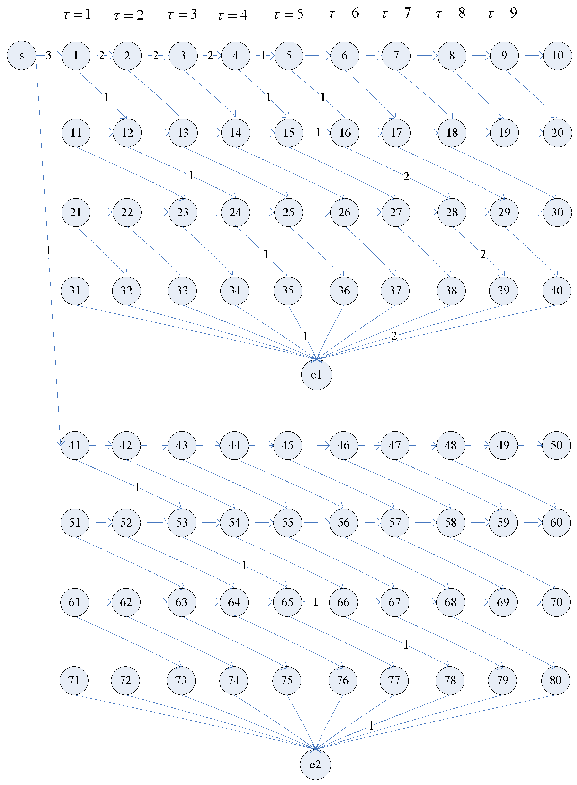
By solving the NOP using the CPLEX problem solver [47], the solution in

Table 4. The solution obtained by solving NOP.

Decision Variable	Value	Decision Variable	Value
$f(s,1)$	3	$f(24,35)$	1
$f(1,2)$	2	$f(28,39)$	2
$f(2,3)$	2	$f(35,e1)$	1
$f(3,4)$	2	$f(39,e1)$	2
$f(4,5)$	1	$f(41,53)$	1
$f(1,12)$	1	$f(53,65)$	1
$f(4,15)$	1	$f(65,66)$	1
$f(5,16)$	1	$f(66,78)$	1
$f(12,24)$	1	$f(78,e2)$	1
$f(16,28)$	2

can be found. Figure 6 represents the solution in the joint spatial temporal network. The value of the objective function of this solution is 0. As the value of objective function is 0, the deadline can be met.

Table 5. The sequence of control actions.

$\mathit{\tau }$	$\mathbf{Control} \mathbf{Action} {\mathit{c}}_{\mathit{\tau }}$	Transitions to Be Fired
1	1 0 0 1 0 0	$t_1$,$t_5$
2	0 1 0 0 0 0	$t_2$
3	0 0 0 0 1 0	$t_6$
4	1 0 1 0 0 0	$t_1$,$t_3$
5	1 0 0 0 0 0	$t_1$
6	0 2 0 0 0 1	$t_2$,$t_2$,$t_3$,$t_7$
7	0 0 0 0 0 0
8	0 0 2 0 0 0	$t_3$,$t_3$
9	0 0 0 0 0 0

shows the sequence of control actions corresponding to the solution in Figure 6. Note that transition $t_1$ is fired three times as the demand for the type-1 product is $D_1$ = 3. Similarly, $t_2$ and $t_3$ are also fired three times as the demand for the type-1 product is $D_1$ = 3. As the demand for the type-2 product is $D_2$ = 1, transitions $t_5$, $t_6$ and $t_7$ are fired one time. The results are consistent with our expectations.

Suppose a type-1 resource failure takes place at place $p_2$ in the first period and is expected to be recovered at the end of the second period. The type-1 resource failure taking place at place $p_2$ can be represented by the perturbation vector $\delta$ = [${\delta }_{r_1}$,${\delta }_{r_2}$,${\delta }_{p_1}$,${\delta }_{p_2}$,…,${\delta }_{p_{10}}$] = [0 1 0 0 0 0 0 0 0 0 0 0] with ${\delta }_{p_2}=1$. The discrete time failure interval for the above-mentioned failure is ${\omega }_{p_{2}1}=[{\alpha }_{p_{2}1}\hspace{0.17em}{\beta }_{p_{2}1}]=[1\hspace{0.17em}2]$ as the failure is expected to last for two periods. The above type-1 resource failure reduces the capacity of type-1 resources. To compute $C_{r\tau }^{\Delta (m)}$, we need the data of ${\mathrm{\Gamma }}_{pr}$ in

Table 6. Data of ${\mathrm{\Gamma }}_{pr}$.

$\mathbf{Place} (\mathit{p})$	$\mathbf{Resource} \mathbf{Type} (\mathit{r})$	${\mathit{\Gamma }}_{\mathit{p}\mathit{r}}$
$p_1$	1	0
$p_2$	1	1
$p_3$	1	0
$p_4$	1	1
$p_5$	1	0
$p_6$	1	0
$p_7$	1	1
$p_8$	1	0
$p_9$	1	1
$p_{10}$	1	0
$r_1$	1	1
$r_2$	1	0
$p_1$	2	0
$p_2$	2	0
$p_3$	2	1
$p_4$	2	0
$p_5$	2	0
$p_6$	2	0
$p_7$	2	0
$p_8$	2	1
$p_9$	2	0
$p_{10}$	2	0
$r_1$	2	0
$r_2$	2	1

.

As the resource failure takes place at place $p_2$ and ${\delta }_{p_2}=1$,

${\mathrm{\Omega }}_{p_{2}1\tau }=1\hspace{0.17em}\forall \tau \in [{\alpha }_{p_{2}1}\hspace{0.17em}{\beta }_{p_{2}1}]=[1\hspace{0.17em}2]$ and ${\mathrm{\Omega }}_{p1\tau }=0$ for $p\ne p_2$. That is, ${\mathrm{\Omega }}_{p_{2}11}={\mathrm{\Omega }}_{p_{2}12}=1$ and ${\mathrm{\Omega }}_{p1\tau }=0$ for $p\ne p_2$. Based on the values of ${\mathrm{\Gamma }}_{pr}$ in Table 6 and the values of $\mathrm{\Omega }$, (7) is applied to compute $C_{r\tau }^{\Delta (m)}$.

Table 7. The capacity of each type of resources in each period after type-1 resource failure.

$\mathbf{Resource} \mathbf{Type} (\mathit{r})$	$\mathbf{Period} (\mathit{t})$	${\mathit{C}}_{\mathit{r}\mathit{\tau }}^{\mathbf{\Delta }(\mathit{m})}$
1	1	0
1	2	0
1	3	2
1	4	1
1	5	1
1	6	1
1	7	1
1	8	0
1	9	2
2	1	2
2	2	2
2	3	1
2	4	1
2	5	2
2	6	0
2	7	0
2	8	2
2	9	2

shows the capacity of each type of resources in each period after type-1 resource failure. Note that $C_{r\tau }^{\Delta (m)}$ is reduced by one for type-1 resources in the first and second periods.

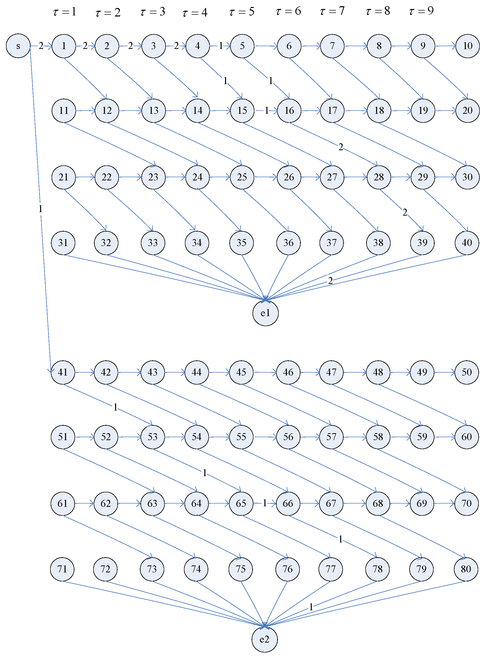
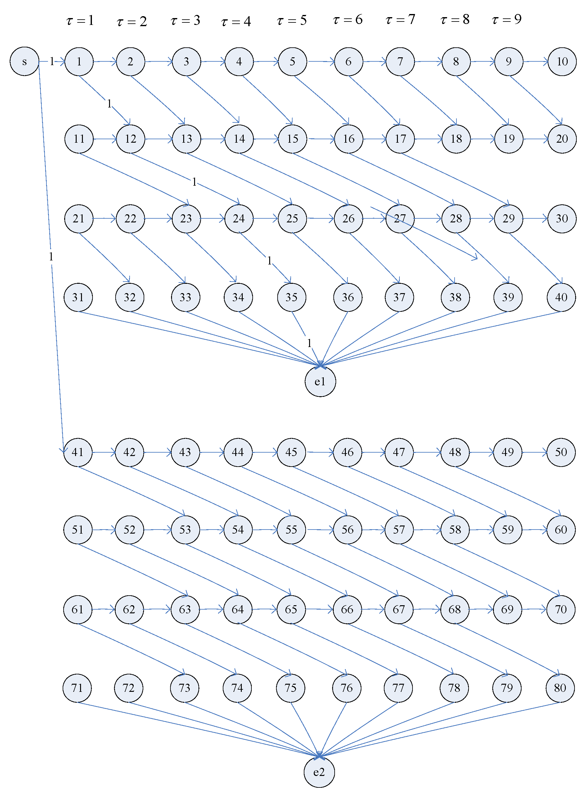
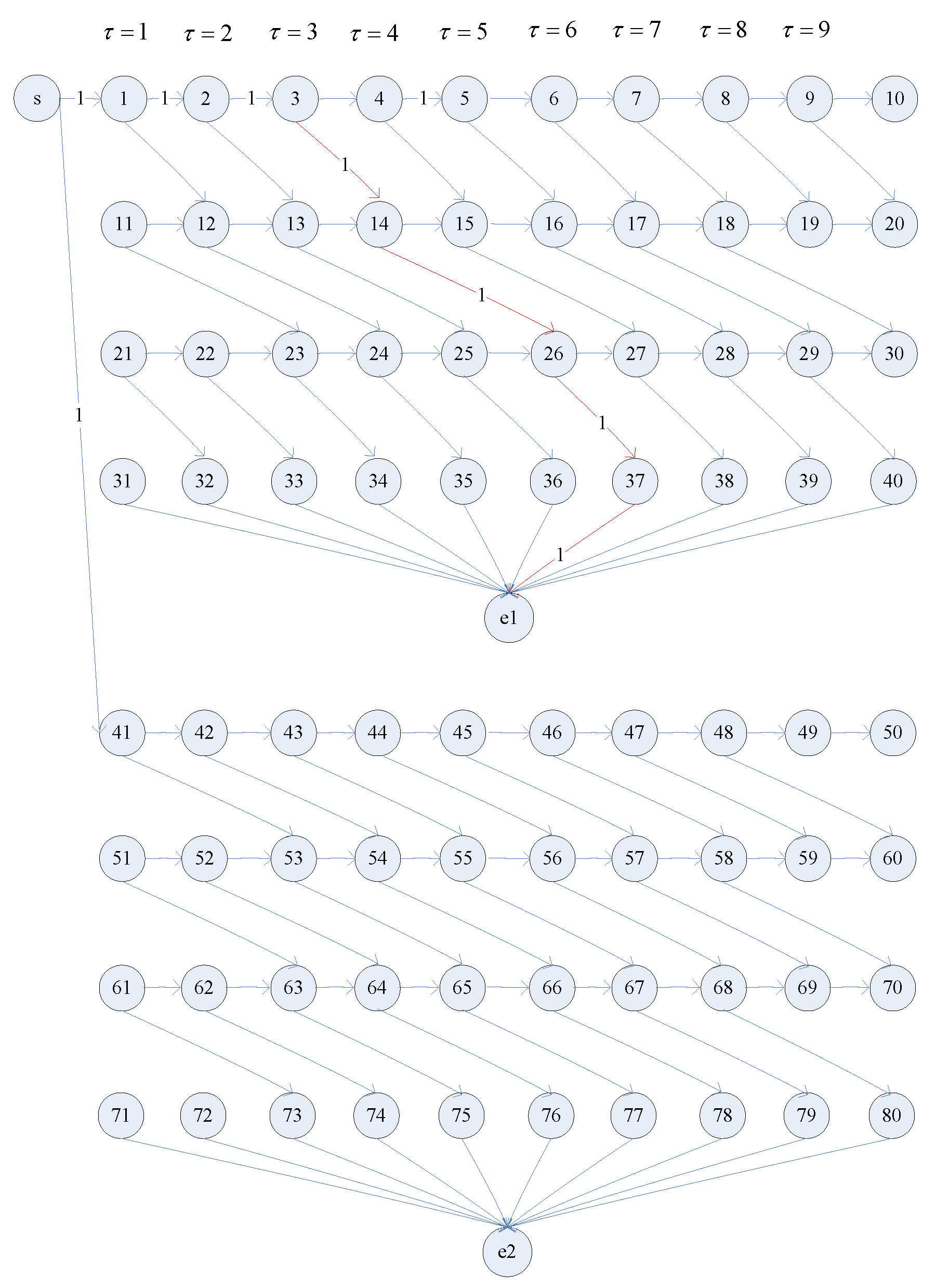
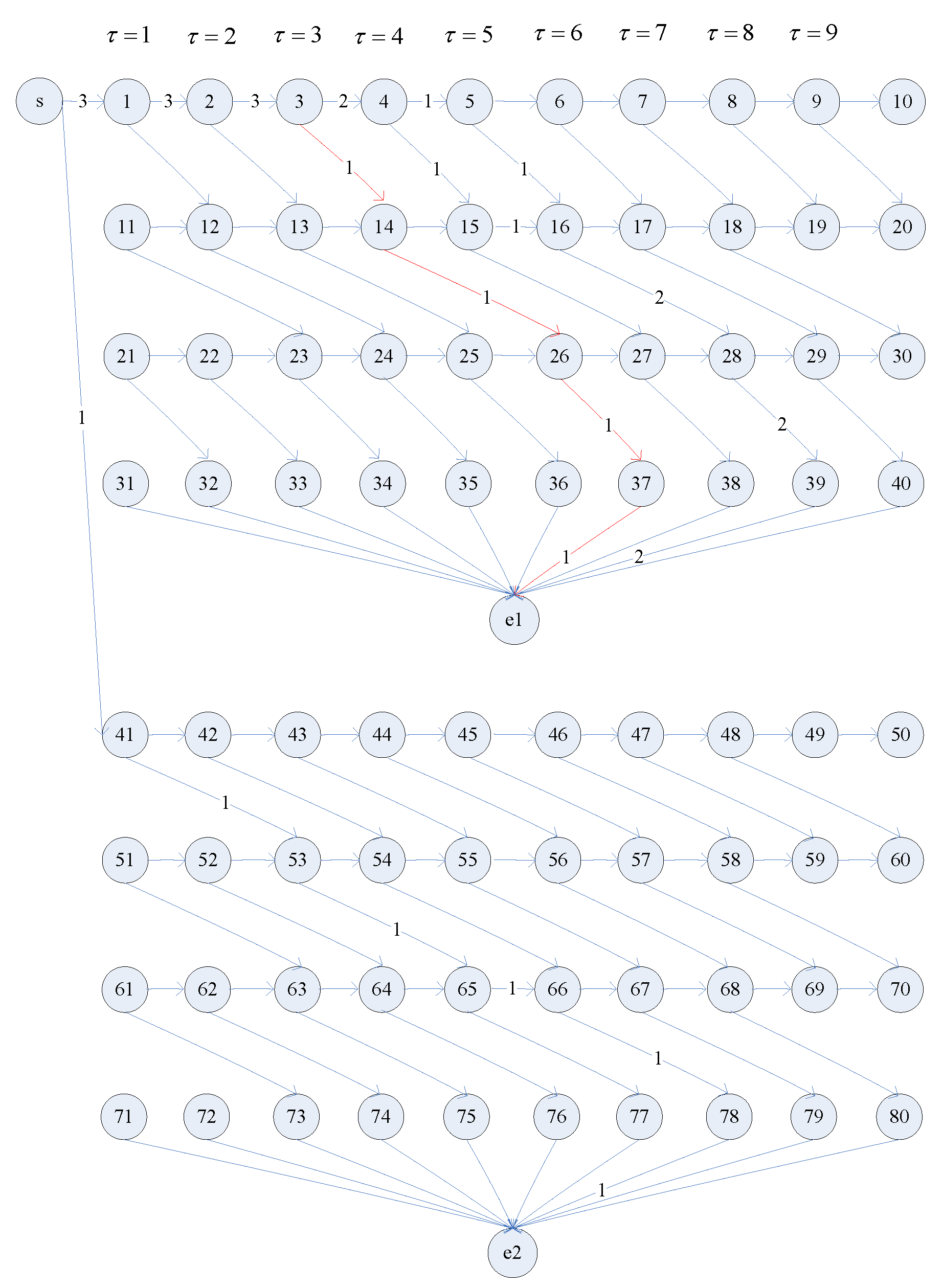
Before solving the ASOP, Algorithm 1 first constructs $JSTN(V,A)$ by applying Procedure 1 in Step1. Next, to deal with $\Delta (m)$ = ($m$,$\delta$,$\omega$), Algorithm 1 divides $f$ into $f_u$ and $f_{\Delta }$ with $f=f_u+f_{\Delta }$ in Step 2 where $f_u$ denotes the flows not influenced by $\Delta (m)$ where as $f_{\Delta }$ denotes the flows influenced by $\Delta (m)$. Instead of listing $f_u$ and $f_{\Delta }$ in tables, to make it clear to illustrate $f_u$ and $f_{\Delta }$, we show $f_u$ and $f_{\Delta }$ in Figure 7 and Figure 8, respectively. Algorithm 1 then applies Procedure 2 to calculate residual capacity ${\tilde{C}}_{rt}$ for $r\in \mathit{R}$ $\forall t\in \{1,2,\dots ,\mathrm{\Pi }\}=\{1,2,\dots ,9\}$ and calculate the quantity of different types of products influenced by $\Delta (m)$. The capacity constraints of the ASOP are defined according to the residual capacity ${\tilde{C}}_{rt}$. In Step 3, Algorithm 1 attempts to find the solution $f_{\Delta }^{\prime }$ for the ASOP defined by $JSTN(V,A)$ with residual capacity constraint ${\tilde{C}}_{rt}$. Figure 9 shows the $f_{\Delta }^{\prime }$ found by solving ASOP. Figure 10 shows the alternative solution $f^{\prime }=f_u+f_{\Delta }^{\prime }$ found by Algorithm 1. Note that the alternative solution $f^{\prime }=f_u+f_{\Delta }^{\prime }$ can still meet the deadline as the objective function value of the solution $f_{\Delta }^{\prime }$ of ASOP is zero.

Table 8. The solution obtained by solving ASOP.

Decision Variable	Value
$f(s,1)$	3
$f(1,2)$	2
$f(2,3)$	1
$f(3,4)$	1
$f(1,12)$	1
$f(2,13)$	1
$f(4,15)$	1
$f(5,16)$	1
$f(12,24)$	1
$f(16,28)$	2
$f(24,35)$	1
$f(28,39)$	2
$f(35,e1)$	1
$f(39,e2)$	2
$f(41,53)$	1
$f(53,65)$	1
$f(65,66)$	1
$f(66,78)$	1
$f(78,e2)$	1

and

Table 9. The sequence of control actions.

$\mathbf{Period} (\mathit{\tau })$	$\mathbf{Control} \mathbf{Action} {\mathit{c}}_{\mathit{\tau }}$	Transitions to Be Fired
1	1 0 0 0 0 0	$t_5$
2	1 1 0 0 0 0
3	0 1 0 0 0 0	$t_1$,$t_6$
4	1 0 0 1 0 0	$t_1$,$t_2$
5	0 1 0 0 0 0	$t_1$
6	0 0 2 0 1 0	$t_2$,,$t_3$,$t_7$
7	0 0 1 0 0 0
8	0 0 0 0 0 1	$t_3$,$t_3$
9	0 0 0 0 0 0

show the solution found and the sequence of control actions. As there exists a solution to ASOP, $G_c=(m_0,u)$ is resilient with respect to $\Delta (m)$. As The objective function value is 0, $G_c=(m_0,u)$ is robust with respect to $\Delta (m)$. That is, the deadline can still be met due to the resource failure.

The sequence of control actions constructed based on the solution in Figure 10 is listed in Table 9.

5.2. Computational Efficiency

To illustrate computational feasibility of the method proposed in this study, we first compared the computation time of our proposed approach with that obtained by applying the existing reachability/coverability graph approach for small examples by changing the number of tokens in some places in Figure 2. We showed that the existing reachability/coverability graph approach suffers from state explosion problem even for small examples. In the next section, we showed that our proposed approach could be applied to large problems.

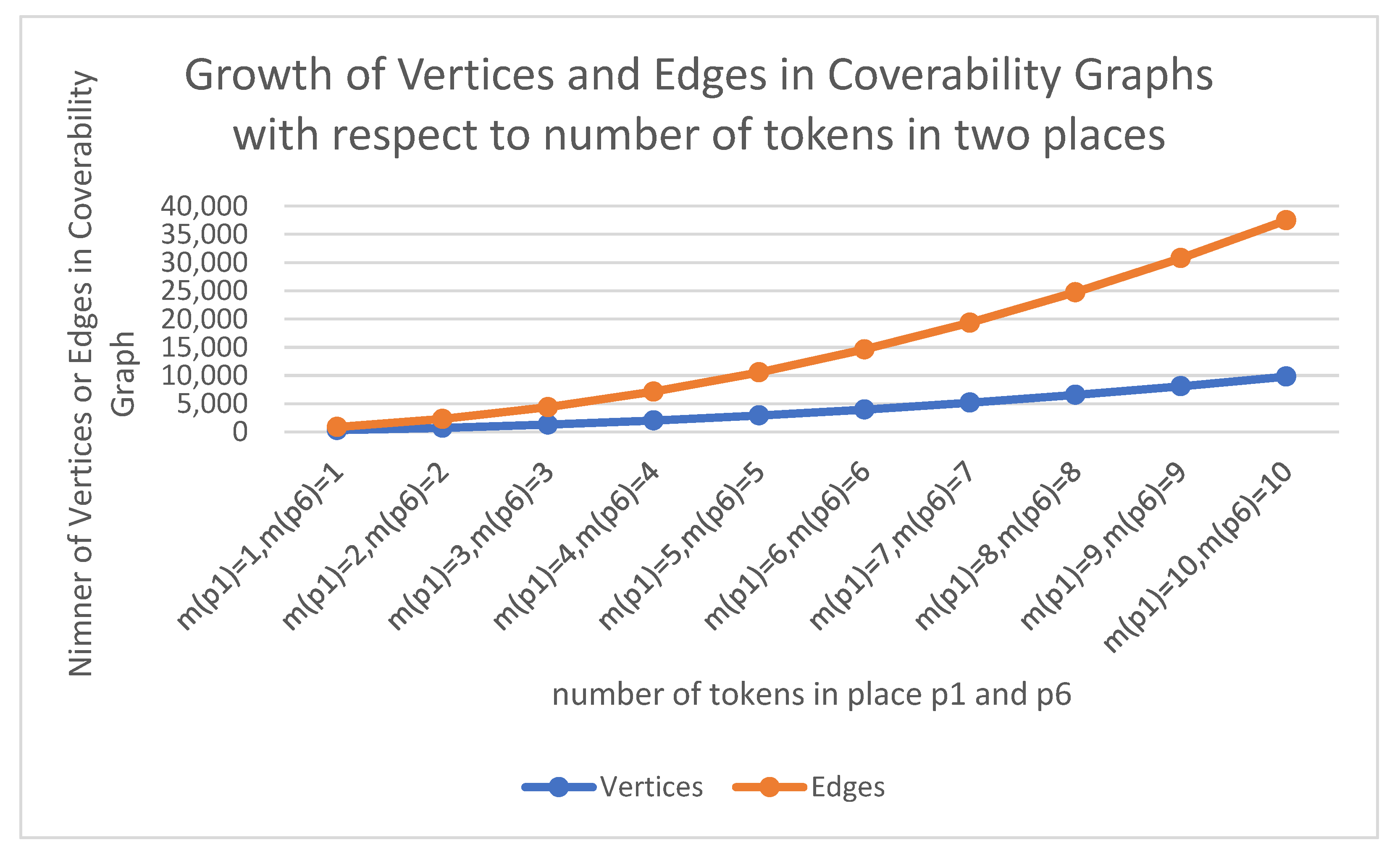
For the example of Figure 2, we increase the number of tokens in place $p_1$ and the number of tokens in place $p_6$ under the initial marking $m_0$ from one to ten, respectively. The numbers of tokens in other places under the initial marking $m_0$ are the same as Figure 2 with the exception of places $p_1$ and $p_6$. The growth of the number of vertices and edges in the coverability graphs is shown in Figure 11. It is clear that the number of vertices and the number of edges in the coverability graphs exponentially grow in Figure 11. The phenomena of state explosion problems can be observed in Figure 11. The state explosion problems mentioned above lead to the exponential growth of computation time for constructing coverability graphs.

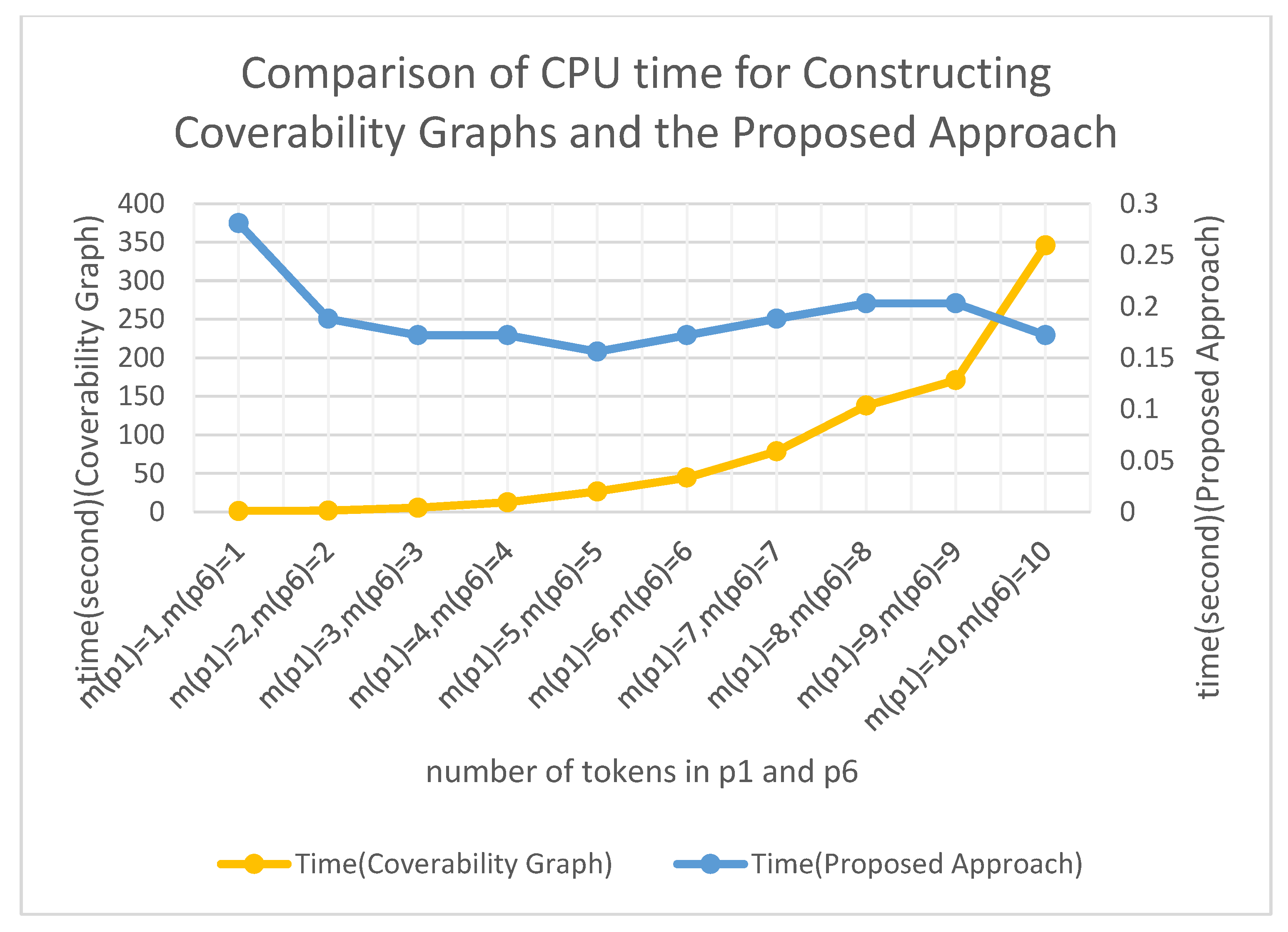
The computation time for constructing coverability graphs and that of the proposed approach is shown in Figure 12. The computation time for constructing coverability graphs is typically over several hundred seconds for most cases, as shown in Figure 12. It takes less than one second for our proposed approach to produce solutions. It is clear that the computation time for constructing coverability graphs exponentially grew in Figure 12 whereas the computation time for the proposed approach did not significantly grow. Obviously, the existing coverability based approach can only be applied to small nets with small numbers of tokens.

The above results indicated that the existing methods based on the construction of coverability graphs were computationally infeasible even for small nets. The above results also showed that our approach was computationally feasible for the small examples above. We illustrate the computational feasibility of the proposed approach in the next section.

5.3. Computationally Feasibility Study

In this section, we present the results of several series of experiments to assess computational feasibility of the proposed method. The experiments were divided into six categories by considering single failure and multiple failures and three problem size parameters. For each category, we generated test cases by increasing the value of one parameter while all the other parameters were fixed. There were three parameters, including the number of operations in a process, time horizon and the number of task types. In addition, the number of failures occurring in cyber-physical production systems was also a parameter for assessment of the computational feasibility of our approach. We classify the experiments into six categories.

The test case data can be downloaded from the following link: https://drive.google.com/drive/folders/1T8LNzxx4BdFalVLA5ZVuvliu6A4Gfp71?usp=sharing (accessed on 1 October 2021).

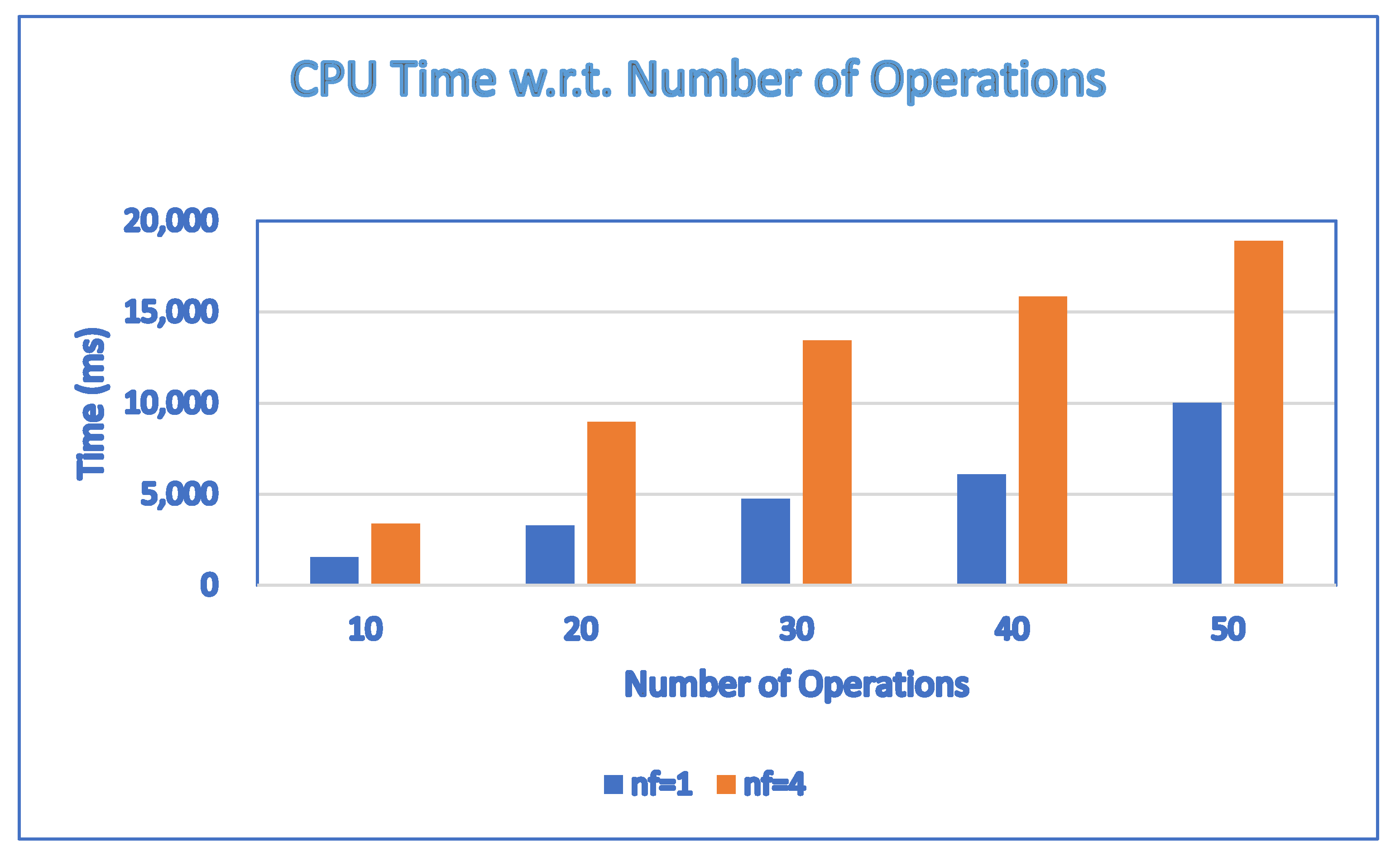
The first category of experiments was to study the computational time for the single failure situation, $nf=1$, where $nf$ denotes the number of failures, by increasing the parameter $K=\underset{j\in \mathit{J}}{\max }\left|T_j\right|$. In this category of experiments, it was assumed that a single failure took place at a single place $p^{\prime }$, with ${\delta }_{p^{\prime }}=1\hspace{0.17em}$ and ${\delta }_p=0\hspace{0.17em}\forall p\in P\backslash \{p^{\prime }\}$. The discrete time failure interval for the above-mentioned failure was ${\omega }_{p^{\prime }1}=[{\alpha }_{p^{\prime }1}\hspace{0.17em}{\beta }_{p^{\prime }1}]$. We conducted a series of experiments by increasing the parameter $K=\underset{j\in \mathit{J}}{\max }\left|T_j\right|$ from 10 to 50 with the other parameters remaining unchanged ($J$ = 4 and $\mathrm{\Pi }$ = 300). In this series of experiments, we set $K$ to be 10, 20, 30, 40 and 50. The results are shown in Figure 11. The results indicated that the CPU time polynomially grew with $K$ for the single failure situation. The results were consistent with the polynomial lower bound $O(\Delta D{(N\mathrm{\Pi }+J)}^2)$ on the complexity to solve the ASOP.

The second category of experiments was to study the computational time for the multiple failures situation, $nf=4$, where $nf$ denotes the number of failures, by increasing the parameter $K=\underset{j\in \mathit{J}}{\max }\left|T_j\right|$. In this category of experiments, it was assumed that four failures took place at four different places: $p_1^{\prime }$,$p_2^{\prime }$,$p_3^{\prime }$ and $p_4^{\prime }$, with ${\delta }_{p^{\prime }}=1\hspace{0.17em}\forall p^{\prime }\in \{p_1^{\prime },p_2^{\prime },p_3^{\prime },p_4^{\prime }\}$ and ${\delta }_{p^{\prime }}=0\forall p^{\prime }\in P\backslash \{p_1^{\prime },p_2^{\prime },p_3^{\prime },p_4^{\prime }\}$. The discrete time failure interval for the above-mentioned failures was ${\omega }_{p^{\prime }1}=[{\alpha }_{p^{\prime }1}\hspace{0.17em}{\beta }_{p^{\prime }1}]$$\forall p^{\prime }\in \{p_1^{\prime },p_2^{\prime },p_3^{\prime },p_4^{\prime }\}$. We conducted a series of experiments by increasing the parameter $K=\underset{j\in \mathit{J}}{\max }\left|T_j\right|$ from 10 to 50 with other parameters remaining unchanged ($J$ = 4 and $\mathrm{\Pi }$ = 300). In this series of experiments, we set  to be 10, 20, 30, 40 and 50. The results are shown in Figure 13. The results were consistent with the polynomial lower bound $O(\Delta D{(N\mathrm{\Pi }+J)}^2)$ on the complexity to solve the ASOP.

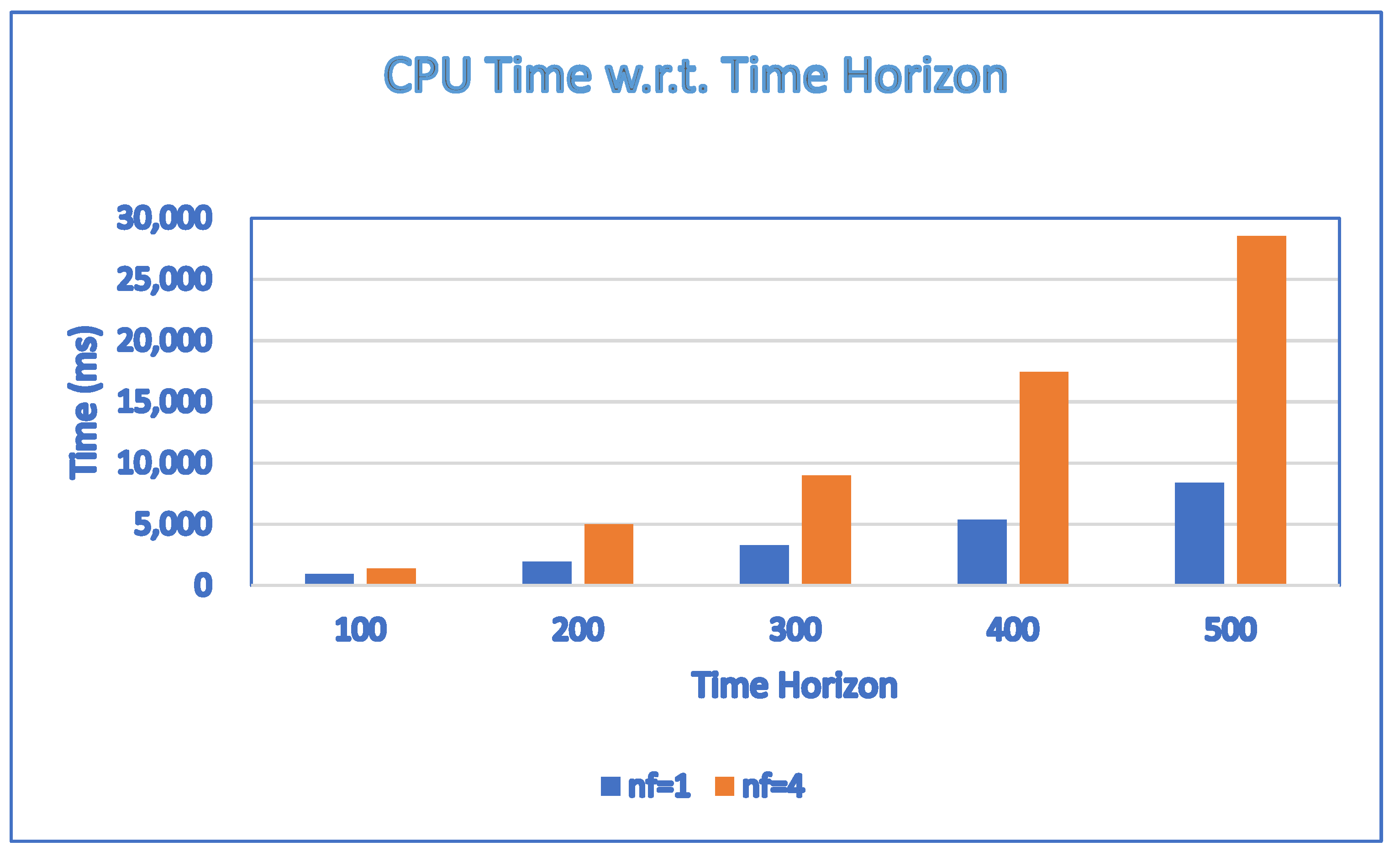
The third category of experiments was to study the computational time for the single failure situation, $nf=1$, where $nf$ denotes the number of failures, by increasing the parameter $\mathrm{\Pi }$. In this category of experiments, it was assumed that a single failure took place at a single place $p^{\prime }$, with ${\delta }_{p^{\prime }}=1\hspace{0.17em}$ and ${\delta }_p=0\hspace{0.17em}\forall p\in P\backslash \{p^{\prime }\}$. The discrete time failure interval for the above-mentioned failure was ${\omega }_{p^{\prime }1}=[{\alpha }_{p^{\prime }1}\hspace{0.17em}{\beta }_{p^{\prime }1}]$. We conducted a series of experiments by changing the parameter $\mathrm{\Pi }$ from 100 to 500 with other parameters remaining unchanged ($J$ = 4 and ${\Pi }$ = 20). In this series of experiments, we set $\mathrm{\Pi }$ to be 100, 200, 300, 400 and 500. The results are shown in Figure 14. The results indicated that the CPU time polynomially grew with $\mathrm{\Pi }$. The results were consistent with the polynomial lower bound $O(\Delta D{(N\mathrm{\Pi }+J)}^2)$ on the complexity to solve ASOP.

The fourth category of experiments was to study the computational time for the multiple failures situation, $nf=4$, where $nf$ denotes the number of failures, by increasing the parameter $\mathrm{\Pi }$. In this category of experiments, it was assumed that four failures took place at four different places $p_1^{\prime }$, $p_2^{\prime }$, $p_3^{\prime }$ and $p_4^{\prime }$, with ${\delta }_{p^{\prime }}=1\hspace{0.17em}\forall p^{\prime }\in \{p_1^{\prime },p_2^{\prime },p_3^{\prime },p_4^{\prime }\}$ and ${\delta }_{p^{\prime }}=0\forall p^{\prime }\in P\backslash \{p_1^{\prime },p_2^{\prime },p_3^{\prime },p_4^{\prime }\}$. The discrete time failure interval for the above-mentioned failures was ${\omega }_{p^{\prime }1}=[{\alpha }_{p^{\prime }1}\hspace{0.17em}{\beta }_{p^{\prime }1}]$$\forall p^{\prime }\in \{p_1^{\prime },p_2^{\prime },p_3^{\prime },p_4^{\prime }\}$. We conducted a series of experiments by changing the parameter $\mathrm{\Pi }$ from 100 to 500 with other parameters remaining unchanged ($J$ = 4 and K = 20). In this series of experiments, we set $\mathrm{\Pi }$ to be 100, 200, 300, 400 and 500. The results are shown in Figure 12. The results indicated that the CPU time polynomially grew with $\mathrm{\Pi }$. The results were consistent with the polynomial lower bound $O(\Delta D{(N\mathrm{\Pi }+J)}^2)$ on the complexity to solve the ASOP.

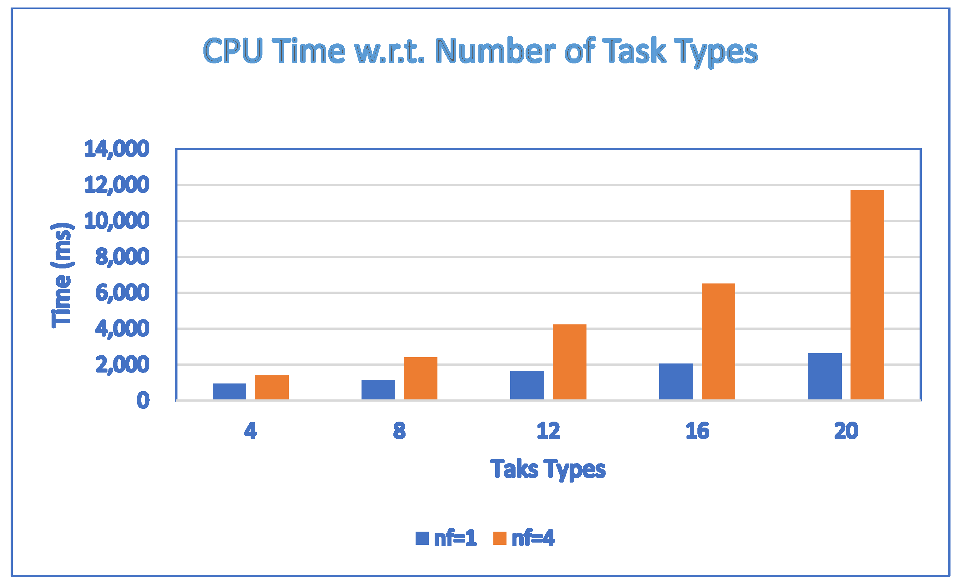
The fifth category of experiments was to study the computational time for the single failure situation, $nf=1$, where $nf$ denotes the number of failures, by increasing the parameter $J$. In this category of experiments, it was assumed that a single failure took place at a single place $p^{\prime }$, with ${\delta }_{p^{\prime }}=1\hspace{0.17em}$ and ${\delta }_p=0\hspace{0.17em}\forall p\in P\backslash \{p^{\prime }\}$. The discrete time failure interval for the above-mentioned failure was ${\omega }_{p^{\prime }1}=[{\alpha }_{p^{\prime }1}\hspace{0.17em}{\beta }_{p^{\prime }1}]$. We conducted a series of experiments by changing the parameter ($J$ from 4 to 20 while keeping other parameters unchanged ($\mathrm{\Pi }$ = 100 and K = 20). In this series of experiments, we set  to be 4, 8, 12, 16 and 20. The results are shown in Figure 15. The results showed that the CPU time polynomially grew with $J$. This was consistent with the polynomial lower bound $O(\Delta D{(N\mathrm{\Pi }+J)}^2)$ on the complexity to solve the ASOP.

The sixth category of experiments was to study the computational time for the multiple failures situation, $nf=4$, where $nf$ denotes the number of failures, by increasing the parameter $J$. In this category of experiments, it was assumed that four failures took place at four different places $p_1^{\prime }$, $p_2^{\prime }$, $p_3^{\prime }$ and $p_4^{\prime }$, with ${\delta }_{p^{\prime }}=1\forall p^{\prime }\in P\backslash \{p_1^{\prime },p_2^{\prime },p_3^{\prime },p_4^{\prime }\}$ and ${\delta }_{p^{\prime }}=0\forall p^{\prime }\in P\backslash \{p_1^{\prime },p_2^{\prime },p_3^{\prime },p_4^{\prime }\}$. The discrete time failure interval for the above-mentioned failures was ${\omega }_{p^{\prime }1}=[{\alpha }_{p^{\prime }1}\hspace{0.17em}{\beta }_{p^{\prime }1}]$$\forall p^{\prime }\in \{p_1^{\prime },p_2^{\prime },p_3^{\prime },p_4^{\prime }\}$. We conducted a series of experiments by changing the parameter $J$ from 4 to 20 while keeping other parameters unchanged ($\mathrm{\Pi }$ = 100 and K = 20). In this series of experiments, we set $J$ to be 4, 8, 12, 16 and 20. The results are shown in Figure 15. The results showed that the CPU time polynomially grew with $J$. This was consistent with the polynomial lower bound $O(\Delta D{(N\mathrm{\Pi }+J)}^2)$ on the complexity to solve the ASOP.

6. Discussion

In this study, we unveiled the development of a theory to assess the robustness and resilience properties of cyber-physical production systems in terms of the ability to meet order demand and timeliness to meet an order due date in the presence of failures of resources. A method was proposed to deal with failures of a class of cyber-physical production systems described by cyber-world models with discrete timed Petri nets. The proposed method was based on transforming discrete timed Petri nets into a joint spatial-temporal network (JSTN) and defining an alternative solution optimization problem (ASOP) based on the joint spatial-temporal network to attempt to search for an alternative solution. In Section 5.1, we illustrated the proposed approach by a small example with a single resource failure in the system to describe the key steps of the proposed solution algorithm. The results of the small example showed the proposed solution algorithm could find an alternative solution to meet product demand of the order. That is, the CPPS was resilient with respect to the single resource failure for the small example. As the due date of the order could be met in the presence of the single resource failure, the CPPS was robust with respect to the resource failure.

In addition to illustration of the proposed approach by a small example, it was important to study whether the approach was scalable with respect to the size of problems with different failures patterns. Scalability aimed to verify whether the proposed approach can efficiently solve a problem in terms of computation time. Existing approaches based on different variants of timed Petri nets can only be applied to small problems and are not scalable as the problem size grew. The results presented in Section 5.2 indicated that the number of vertices and edges of the coverability graphs used in existing approach exponentially grew, which led to the state explosion problem and exponential growth of computation time. The computation time for constructing coverability graphs was typically over several hundred seconds for most cases in Section 5.2 whereas it took less than one second for our proposed approach to produce solutions. The computation time for constructing coverability graphs exponentially grew whereas the computation time for our proposed approach did not significantly grow. The existing coverability based approach could only be applied to small nets with small numbers of tokens.

The proposed approach was different from the existing ones as it did not rely on the variants of approaches based on the concept of state classes as seen in the literature. To study the scalability of the proposed approach, we performed experiments to assess the computational efficiency of the proposed algorithms by applying the proposed algorithm. We considered two types of failure modes, single and multiple failures, in our experiments. As there were three problem size parameters, we considered three types of test cases for each failure mode. For each type of failure mode, we created test cases by increasing the value of one parameter while all the other parameters were fixed. As a result, the overall experiments were divided into six (=2 × 3) categories. The results for all these six categories were presented in Section 5.3. For all test cases, the solutions could be efficiently obtained in less than 30 s by using a laptop. This indicated that the method proposed in this study was computationally feasible for solving real problems.

The way to construct a Petri net model for a real system depends on the level of details to be modelled. A transition in a Petri net model is used to model an event that might take place in a real system. For example, in scheduling problems, one primarily cares about the assignment of resources to tasks to perform operations. In this case, the transitions in the Petri net model correspond to allocation and de-allocation events. If more details about the events between an allocation and a de-allocation event are needed, one may insert one or more transitions between the allocation event and the de-allocation event to obtain a Petri net model with more details. As the structure of the resulting detailed Petri net is still a sequential structure, our method can still be applied to the detailed Petri net.

7. Conclusions

Resilience is the capability to recover quickly from difficulties or changes to meet the goals as much as possible through the implementation of effective schemes or strategies and successfully adapt to challenging situations. It is an important property for enterprises to survive in a dynamically changing business environment. Robustness refers to the ability to tolerate perturbations. It is an important property for enterprises to achieve their original goals in the presence of uncertainties such as resource failures. Resilience and robustness are two important properties to determine whether cyber-physical production systems are able to meet order demand, order due date and find an alternative solution in case resource failures occur. In our previous work, the resilience and robustness properties of cyber-physical production systems were not explored. In this study, we studied the resilience and robustness properties of cyber-physical production systems.

In this study, we developed a method to evaluate the influence of resource failures on cyber-physical production systems based on the concept of robustness and resilience. We used a class of discrete timed Petri nets as the cyber-world models of cyber-physical production systems. We introduced an uncertainty model to capture resource failures in cyber-physical production systems described by discrete timed Petri nets. CPPS was resilient with respect to resource failures if there exists a control policy under which the discrete timed Petri net models of CPPS can reach the goal state after the deadline in the presence of resource failures. A CPPS is robust with respect to resource failures if there exists a control policy under which the discrete timed Petri net models of CPPS can reach the goal state by the deadline in the presence of resource failures. We characterized the robustness and resilience properties of cyber-physical production systems with respect to the failures of resources by analyzing the properties of the proposed models. The discrete timed Petri nets were transformed into a joint spatial-temporal network to formulate an alternative solution optimization problem (ASOP) to facilitate the determination of the validity of the robustness and resilience properties of cyber-physical production systems with respect to the failures of resources. We analyzed the complexity of the proposed method and conducted experiments to illustrate the computational feasibility of the proposed method.

The proposed approach is different from the existing ones as it does not rely on the variants of approaches based on the concept of state classes as seen in the literature. We illustrated the proposed method by a small example. To assess the computational feasibility of the proposed method, six categories of experiments were performed. For all test cases, the solutions could be efficiently obtained in less than 30 s by using a laptop. This confirmed the computational feasibility of the proposed approach. The results of the experiments showed that the JSTN model created by the fusion of asymmetrically decomposed STN models of tasks significantly improved the efficiency of the solution algorithm. In this study, we considered a subclass of discrete timed Petri nets to develop a theory and an algorithm to verify the resilience and robustness properties of cyber-physical production systems by exploiting the net structure. An interesting future research direction is to study the resilience and robustness properties of a more general class of discrete timed Petri nets for cyber-physical production systems. According to Wikipedia and the literature, “robustness” refers to the ability to tolerate perturbations that might affect the system’s functional body. The robustness property studied in this study is similar to the one stated on Wikipedia and in the literature. In this study, we only analyzed the robustness and resilience properties of CPPS with respect to the failures of resources. Studies of other robustness and resilience properties of CPPS with respect to other types of uncertainties unexplored in this study are interesting future research directions.

References

- National Institute of Standards and Technology. Workshop Report on Foundations for Innovation in Cyber-Physical Systems, January 2013. Available online: https://www.nist.gov/el/cyber-physical-systems (accessed on 2 October 2022).
- Al-Ali, R.; Bulej, L.; Kofroň, J.; Bureš, T. A guide to design uncertainty-aware self-adaptive components in Cyber–Physical Systems. Future Gener. Comput. Syst. 2022, 128, 466–489. [Google Scholar] [CrossRef]
- Nguyen, W.P.V.; Nair, A.S.; Nof, S.Y. Advancing Cyber-Physical Systems Resilience: The Effects of Evolving Disruptions. Procedia Manuf. 2019, 39, 334–340. [Google Scholar] [CrossRef]
- Du, D.; Huang, P.; Jiang, K.; Mallet, F. pCSSL: A stochastic extension to MARTE/CCSL for modeling uncertainty in Cyber Physical Systems. Sci. Comput. Program. 2018, 166, 71–88. [Google Scholar] [CrossRef]
- Zhu, B.; Wang, Y.; Zhang, H.; Xie, X. Distributed finite-time fault estimation and fault-tolerant control for cyber-physical systems with matched uncertainties. Appl. Math. Comput. 2021, 403, 126195. [Google Scholar] [CrossRef]
- Hosseinzadeh, M.; Sinopoli, B. Active Attack Detection and Control in Constrained Cyber-Physical Systems Under Prevented Actuation Attack. In Proceedings of the 2021 American Control Conference (ACC), New Orleans, LA, USA, 25–28 May 2021; pp. 3242–3247. [Google Scholar]
- Griffioen, P.; Romagnoli, R.; Krogh, B.H.; Sinopoli, B. Resilient Control in the Presence of Man-in-the-Middle Attacks. In Proceedings of the 2021 American Control Conference (ACC), New Orleans, LA, USA, 25–28 May 2021; pp. 4553–4560. [Google Scholar]
- Zhang, M.; Yue, T.; Ali, S.; Selic, B.; Okariz, O.; Norgre, R.; Intxausti, K. Specifying uncertainty in use case models. J. Syst. Softw. 2018, 144, 573–603. [Google Scholar] [CrossRef]
- Bureš, T.; Hnětynka, P.; Plášil, F.; Škoda, D.; Kofroň, J.; Ali, R.A.; Gerostathopoulos, I. Targeting uncertainty in smart CPS by confidence-based logic. J. Syst. Softw. 2021, 181, 111065. [Google Scholar] [CrossRef]
- Cámara, J.; Garlan, D.; Kang, W.G.; Peng, W.; Schmerl, B. Uncertainty in Self-Adaptive Systems Categories Management and Perspectives, CMU-ISR-17-110, School of Computer Science, Carnegie Mellon University, July 2017. Available online: https://reports-archive.adm.cs.cmu.edu/anon/isr2017/CMU-ISR-17-110.pdf (accessed on 2 October 2022).
- Shin, S.Y.; Chaouch, K.; Nejati, S.; Sabetzadeh, M.; Briand, L.C.; Zimmer, F. Uncertainty-aware specification and analysis for hardware-in-the-loop testing of cyber-physical systems. J. Syst. Softw. 2021, 171, 110813. [Google Scholar] [CrossRef]
- Hu, F.; Lu, Y.L.; Vasilakos, A.V.; Hao, Q.; Ma, R.; Patil, Y.; Zhang, T.; Lu, J.; Li, X.; Xiong, N.N. Robust Cyber-Physical Systems: Concept, models, and implementation. Future Gener. Comput. Syst. 2016, 56, 449–475. [Google Scholar] [CrossRef] [Green Version]
- Bennaceur, A.; Ghezzi, C.; Tei, K.; Kehrer, T.; Weyns, D.; Calinescu, R.; Dustdar, S.; Hu, Z.; Honiden, S.; Ishikawa, F.; et al. Modelling and Analysing Resilient Cyber-Physical Systems. In Proceedings of the 2019 IEEE/ACM 14th International Symposium on Software Engineering for Adaptive and Self-Managing Systems (SEAMS), Montreal, QC, Canada, 25–26 May 2019; pp. 70–76. [Google Scholar] [CrossRef] [Green Version]
- Hsieh, F.S. A Dynamic Context-Aware Workflow Management Scheme for Cyber-Physical Systems Based on Multi-Agent System Architecture. Appl. Sci. 2021, 11, 2030. [Google Scholar] [CrossRef]
- Hsieh, F.S. Robust Supervisory Control for Cyber-Physical Systems based on Discrete Timed Petri nets. In Proceedings of the 2022 IEEE 12th Annual Computing and Communication Workshop and Conference (CCWC), Virtual, 26–29 January 2022; pp. 1–6. [Google Scholar]
- Hsieh, F.S. Robustness Analysis for a Class of Cyber-Physical Systems modeled with Discrete Timed Petri Nets. In Proceedings of the 2022 IEEE 13th Annual Information Technology, Electronics, and Mobile Communication Conference (IEMCON 2022), Online, 12–15 October 2022; pp. 1–6. [Google Scholar]
- Murata, T. Petri nets: Properties, analysis and applications. Proc. IEEE 1989, 77, 541–580. [Google Scholar] [CrossRef]
- Hsieh, F.-S. Temporal Analysis of Influence of Resource Failures on Cyber-Physical Systems Based on Discrete Timed Petri Nets. Appl. Sci. 2021, 11, 6469. [Google Scholar] [CrossRef]
- Hsieh, F.-S. A Theoretical Foundation for Context-Aware Cyber-Physical Production Systems. Appl. Sci. 2022, 12, 5129. [Google Scholar] [CrossRef]
- Sampigethaya, K.; Poovendran, R. Cyber-physical integration in future aviation information systems. In Proceedings of the 2012 IEEE/AIAA 31st Digital Avionics Systems Conference (DASC), Williamsburg, VA, USA, 14–18 October 2012; pp. 7–12. [Google Scholar]
- Banerjee, A.; Venkatasubramanian, K.K.; Mukherjee, T.; Gupta, S.K.S. Ensuring Safety, Security, and Sustainability of Mission-Critical Cyber–Physical Systems. Proc. IEEE 2012, 100, 283–299. [Google Scholar] [CrossRef]
- Taneja, J.; Katz, R.; Culler, D. Defining CPS Challenges in a Sustainable Electricity Grid. In Proceedings of the 2012 IEEE/ACM Third International Conference on Cyber-Physical Systems, Beijing, China, 17–19 April 2012; pp. 119–128. [Google Scholar]
- Lee, I.; Sokolsky, O.; Chen, S.; Hatcliff, J.; Jee, E.; Kim, B.G.; King, A.; Mullen-Fortino, M.; Park, S.; Roederer, A.; et al. Challenges and Research Directions in Medical Cyber–Physical Systems. Proc. IEEE 2012, 100, 75–90. [Google Scholar]
- Monostori, L. Cyber-physical Production Systems: Roots, Expectations and R&D Challenges. Procedia CIRP 2014, 17, 9–13. [Google Scholar]
- Li, X.; Qiao, C.; Wagh, A.; Sudhaakar, R.; Addepalli, S.; Wu, C.; Sadek, A. A Holistic Approach to Service Delivery in Driver-in-the-Loop Vehicular CPS. IEEE J. Sel. Areas Commun. 2013, 31, 513–522. [Google Scholar]
- Schirner, G.; Erdogmus, D.; Chowdhury, K.; Padir, T. The Future of Human-in-the-Loop Cyber-Physical Systems. Computer 2013, 46, 36–45. [Google Scholar] [CrossRef]
- Nandhini, R.S.; Lakshmanan, R. A Review of the Integration of Cyber-Physical System and Internet of Things. Int. J. Adv. Comput. Sci. Appl. 2022, 13, 459–465. [Google Scholar] [CrossRef]
- Derler, P.; Lee, E.A.; Vincentelli, A.S. Modeling Cyber–Physical Systems. Proc. IEEE 2012, 100, 13–28. [Google Scholar] [CrossRef]
- Aguida, M.A.; Ouchani, S.; Benmalek, M. A Review on Cyber-Physical Systems: Models and Architectures. In Proceedings of the 2020 IEEE 29th International Conference on Enabling Technologies: Infrastructure for Collaborative Enterprises (WETICE), Bayonne, France, 10–13 September 2020; pp. 275–278. [Google Scholar]
- Lozano, C.V.; Vijayan, K.K. Literature review on Cyber Physical Systems Design. Procedia Manuf. 2020, 45, 295–300. [Google Scholar] [CrossRef]
- Sharma, D.M.; Shandilya, S.K.; Sharma, A.K. A Comprehensive Review on Cyber Physical System and Its Applications in Robotic Process Automation. In Innovations in Bio-Inspired Computing and Applications. IBICA 2020. Advances in Intelligent Systems and Computing; Abraham, A., Sasaki, H., Rios, R., Gandhi, N., Singh, U., Ma, K., Eds.; Springer: Cham, Switzerland, 2021; Volume 1372, pp. 311–312. [Google Scholar]
- Liu, Y.; Peng, Y.; Wang, B.; Yao, S.; Liu, Z. Review on cyber-physical systems. IEEE/CAA J. Autom. Sin. 2017, 4, 27–40. [Google Scholar] [CrossRef]
- Koutsoukos, X.; Karsai, G.; Laszka, A.; Neema, H.; Potteiger, B.; Volgyesi, P.; Vorobeychik, Y.; Sztipanovits, J. SURE: A Modeling and Simulation Integration Platform for Evaluation of Secure and Resilient Cyber–Physical Systems. Proc. IEEE 2018, 106, 93–112. [Google Scholar] [CrossRef]
- Galaske, N.; Anderl, R. Disruption Management for Resilient Processes in Cyber-physical Production Systems. Procedia CIRP 2016, 50, 442–447. [Google Scholar] [CrossRef] [Green Version]
- Tomiyama, T.; Moyen, F. Resilient architecture for cyber-physical production systems. CIRP Ann. 2018, 67, 161–164. [Google Scholar] [CrossRef]
- Krishnamurthy, P.; Khorrami, F. Resilient redundancy-based control of cyber-physical systems through adaptive randomized switching. Syst. Control Lett. 2021, 158, 105066. [Google Scholar] [CrossRef]
- Alho, P.; Mattila, J. Service-oriented approach to fault tolerance in CPSs. J. Syst. Softw. 2015, 105, 1–17. [Google Scholar] [CrossRef]
- Jensen, K. Coloured Petri nets. Lect. Notes Comput. Sci. 1987, 254, 248–299. [Google Scholar]
- Popova-Zeugmann, L. Time Petri Nets. In Time and Petri Nets; Springer: Berlin/Heidelberg, Germany, 2013; pp. 31–137. [Google Scholar]
- Holliday, M.A.; Vernon, M.K. A Generalized Timed Petri Net Model for Performance Analysis. IEEE Trans. Softw. Eng. 1987, 12, 1297–1310. [Google Scholar] [CrossRef] [Green Version]
- Giglio, D. Definitions and applications of deterministic-timed Petri nets (DTPN). In Proceedings of the 2006 IEEE International Conference on Systems, Man and Cybernetics, Taipei, Taiwan, 8–11 October 2006; pp. 3060–3067. [Google Scholar]
- Wang, J. Stochastic Timed Petri Nets and Stochastic Petri Nets. In Timed Petri Nets. The Kluwer International Series on Discrete Event Dynamic Systems; Springer: Boston, MA, USA, 1998; Volume 9, pp. 125–153. [Google Scholar]
- Lefebvre, D.; Daoui, C. Control Design for Bounded Partially Controlled TPNs Using Timed Extended Reachability Graphs and MDP. IEEE Trans. Syst. Man Cybern. Syst. 2020, 50, 2273–2283. [Google Scholar] [CrossRef]
- Berthomieu, B.; Menasche, M. An Enumerative Approach for Analyzing Time Petri Nets. In Proceedings of the IFIP Congress, Paris, France, 19–23 September 1983; pp. 41–46. [Google Scholar]
- Klai, K.; Aber, N.; Petrucci, L. A New Approach to Abstract Reachability State Space of Time Petri Nets. In Proceedings of the 2013 20th International Symposium on Temporal Representation and Reasoning, Washington, DC, USA, 26–28 September 2013; pp. 117–124. [Google Scholar]
- Lefebvre, D. Approximated Timed Reachability Graphs for the robust control of discrete event systems. Discret. Event Dyn. Syst. 2019, 29, 31–56. [Google Scholar] [CrossRef]
- CPLEX Optimizer. Available online: https://www.ibm.com/analytics/cplex-optimizer (accessed on 28 February 2022).
Figure 1.
Examples of and ={1,2} and and ={1,2}: (a) ; (b) ; (c) ; (d) .
Figure 2.
Overall model obtained by merging Figure 1a–d (Reprinted with permission from Ref. [19]. Copyright 2022, Fu-Shiung Hsieh).
Figure 3.
An example of the class of models proposed in [18] extended with source and sink transitions (Reprinted with permission from Ref. [19]. Copyright 2022, Fu-Shiung Hsieh).
Figure 4.
(a) An undesirable state in which no transition could be fired any longer; (b) a nominal cyber world model of CPPS in which firing transitions and required allocation of multiple resources (one type-1 and one type-3 resource).
Figure 5.
An example of JSTN.
Figure 6.
A solution of NOP represented in JSTN.
Figure 7.
A sub-solution of NOP represented in JSTN.
Figure 8.
Figure 9.
Figure 10.
A solution of ASOP represented in JSTN.
Figure 11.
Growth of the number of vertices and edges in the coverability graphs.
Figure 12.
Comparison of the computation time.
Figure 13.
CPU time with respect to the number of operations.
Figure 14.
CPU time with respect to time horizon.
Figure 15.
CPU time with respect to number of task types.