
Remaining Useful Life Prediction Method for High Temperature Blades of Gas Turbines Based on 3D Reconstruction and Machine Learning Techniques

Abstract
:1. Introduction
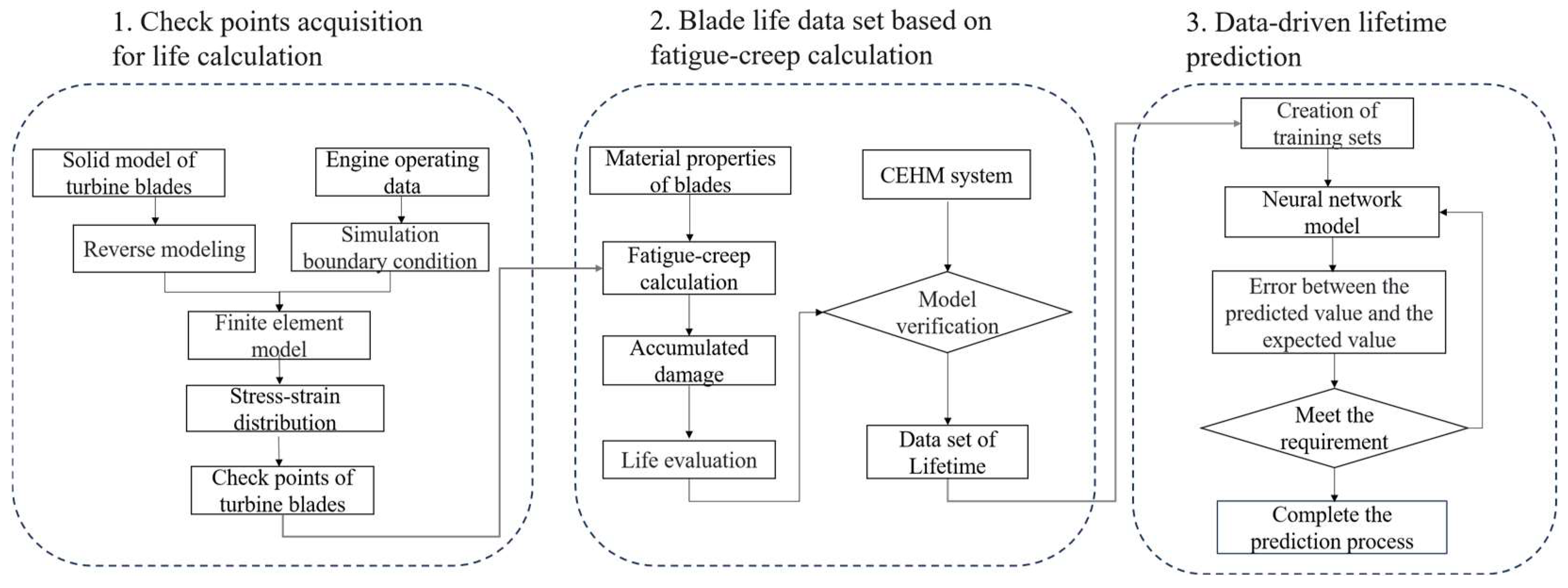
2. Methodology
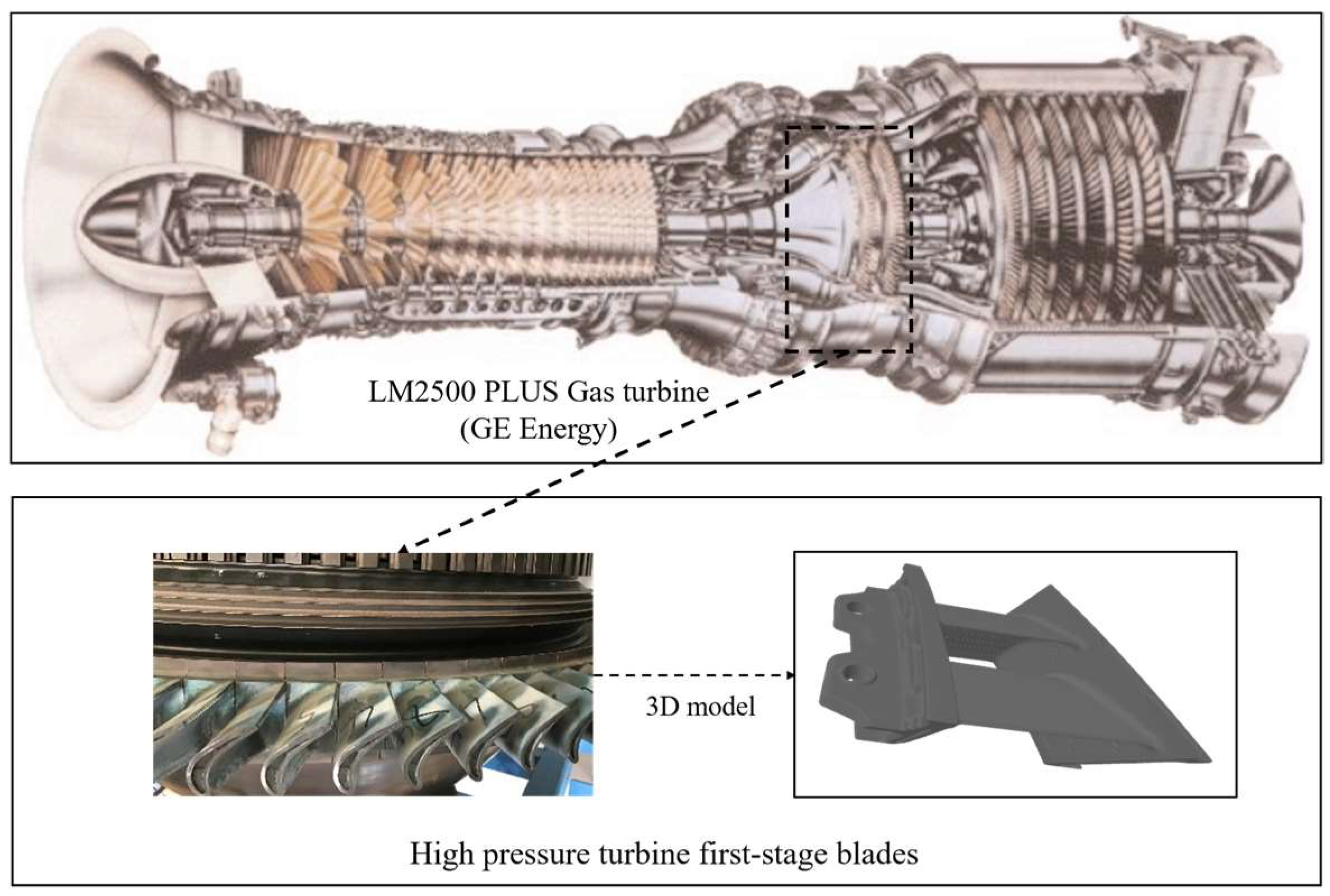
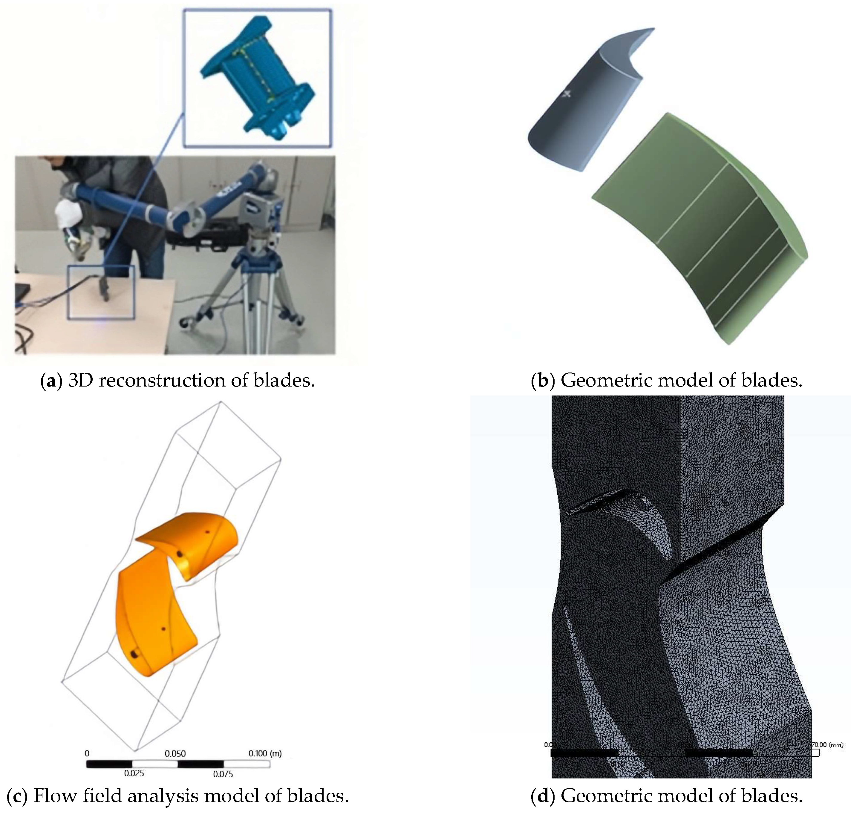
2.1. Reconstructed Geometric Model of the Turbine Blade Based on 3D Scanning Data
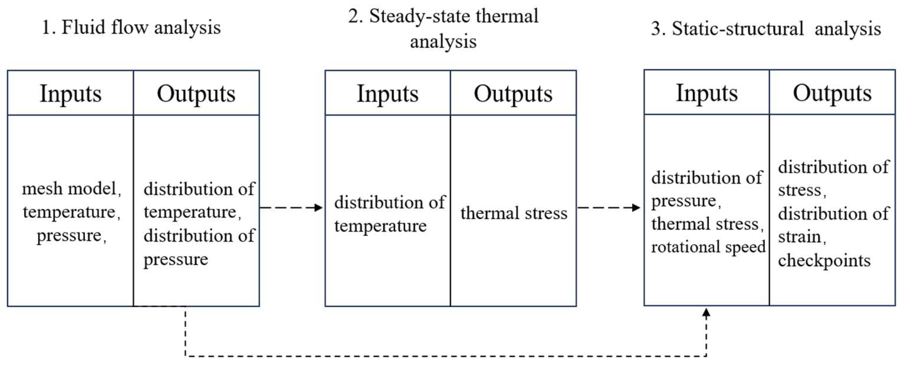
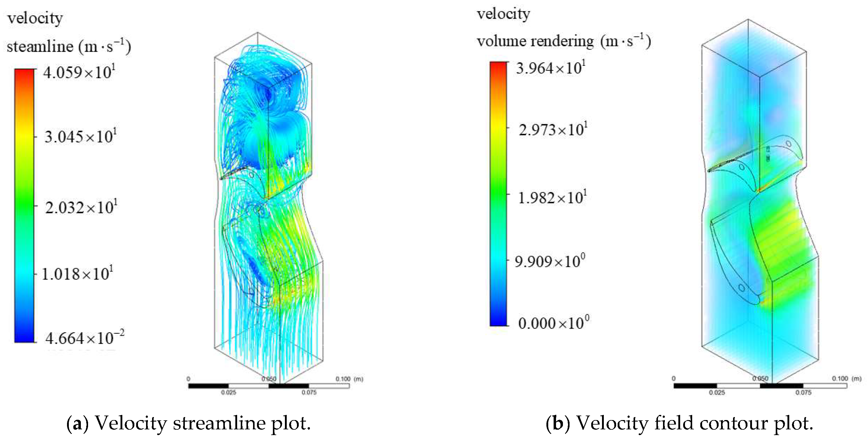
2.2. Three-Dimensional Numerical Simulation
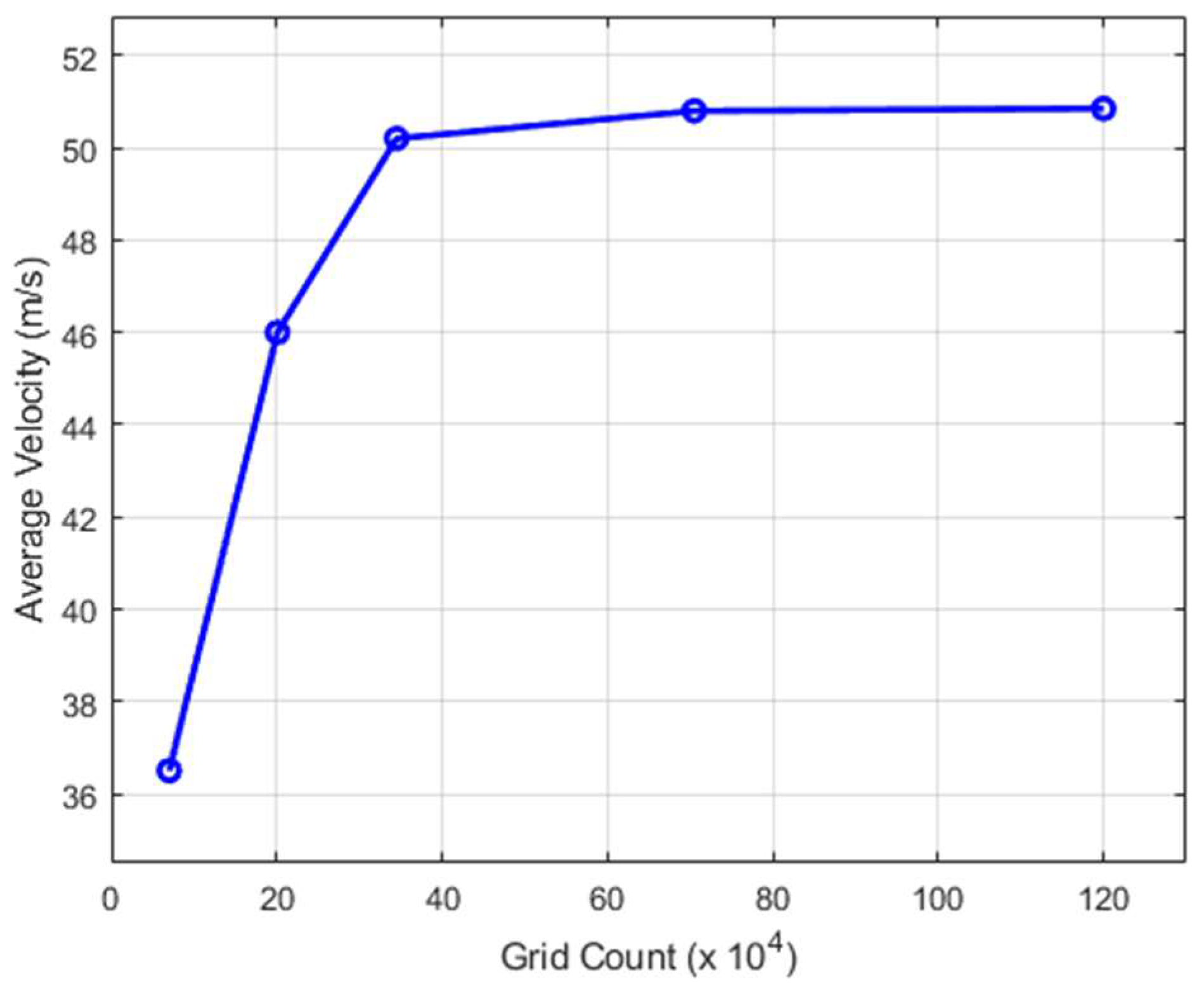
2.2.1. Numerical Methods in Simulation
2.2.2. Governing Equations and Boundary Conditions
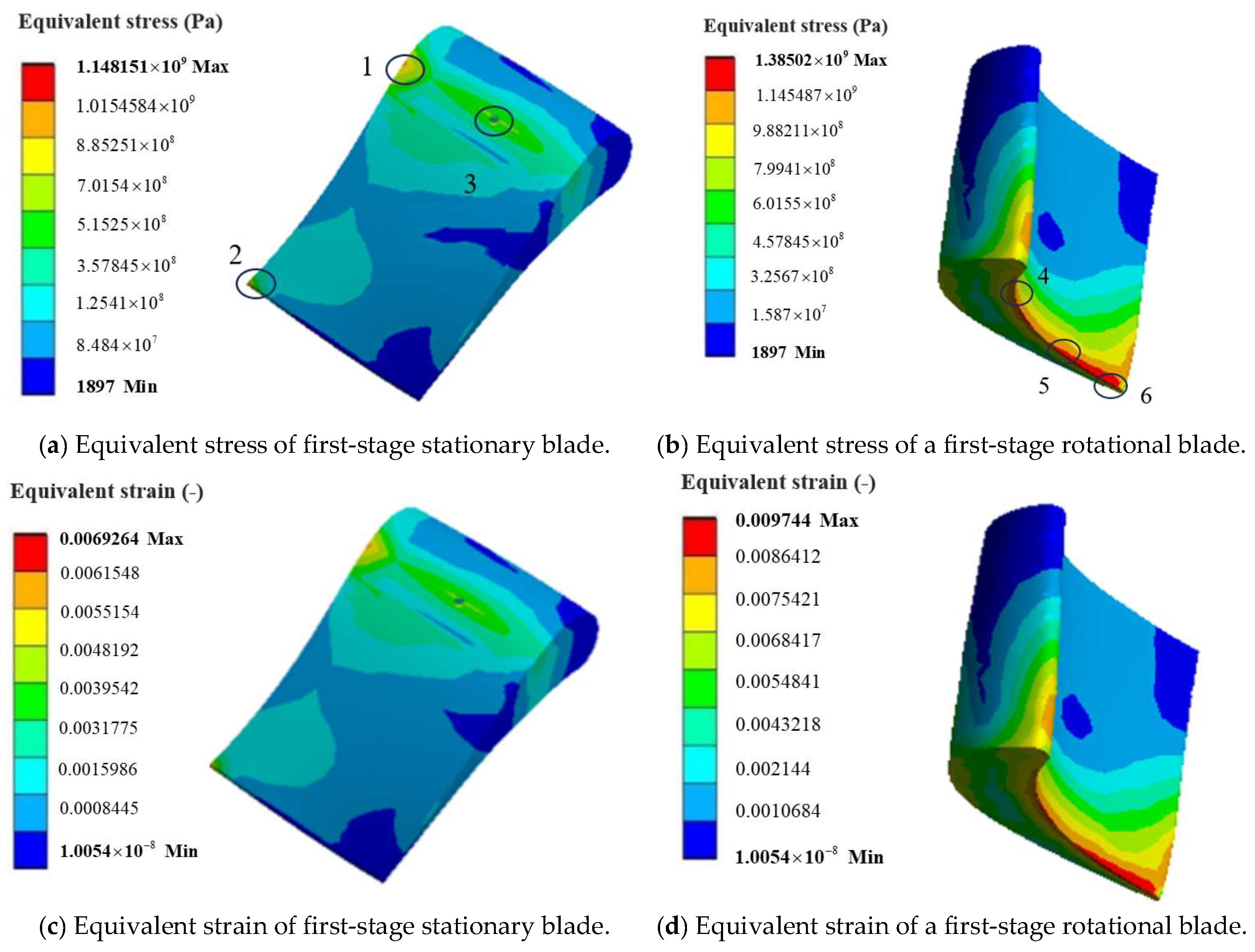
2.2.3. Selection of Checkpoints
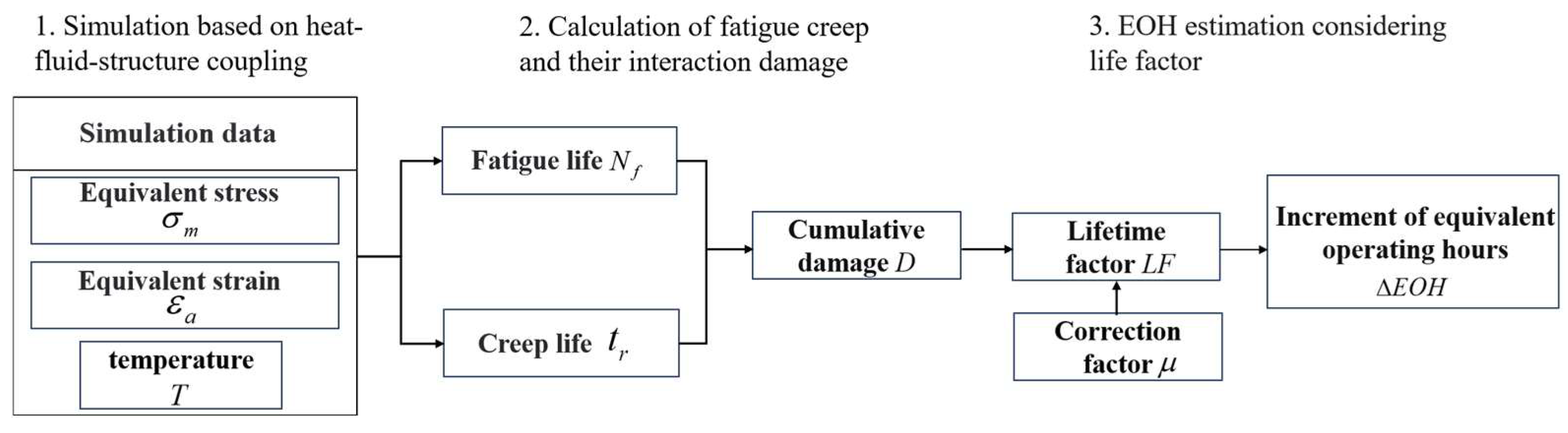
2.3. Data Set of Fatigue-Creep Lifetime
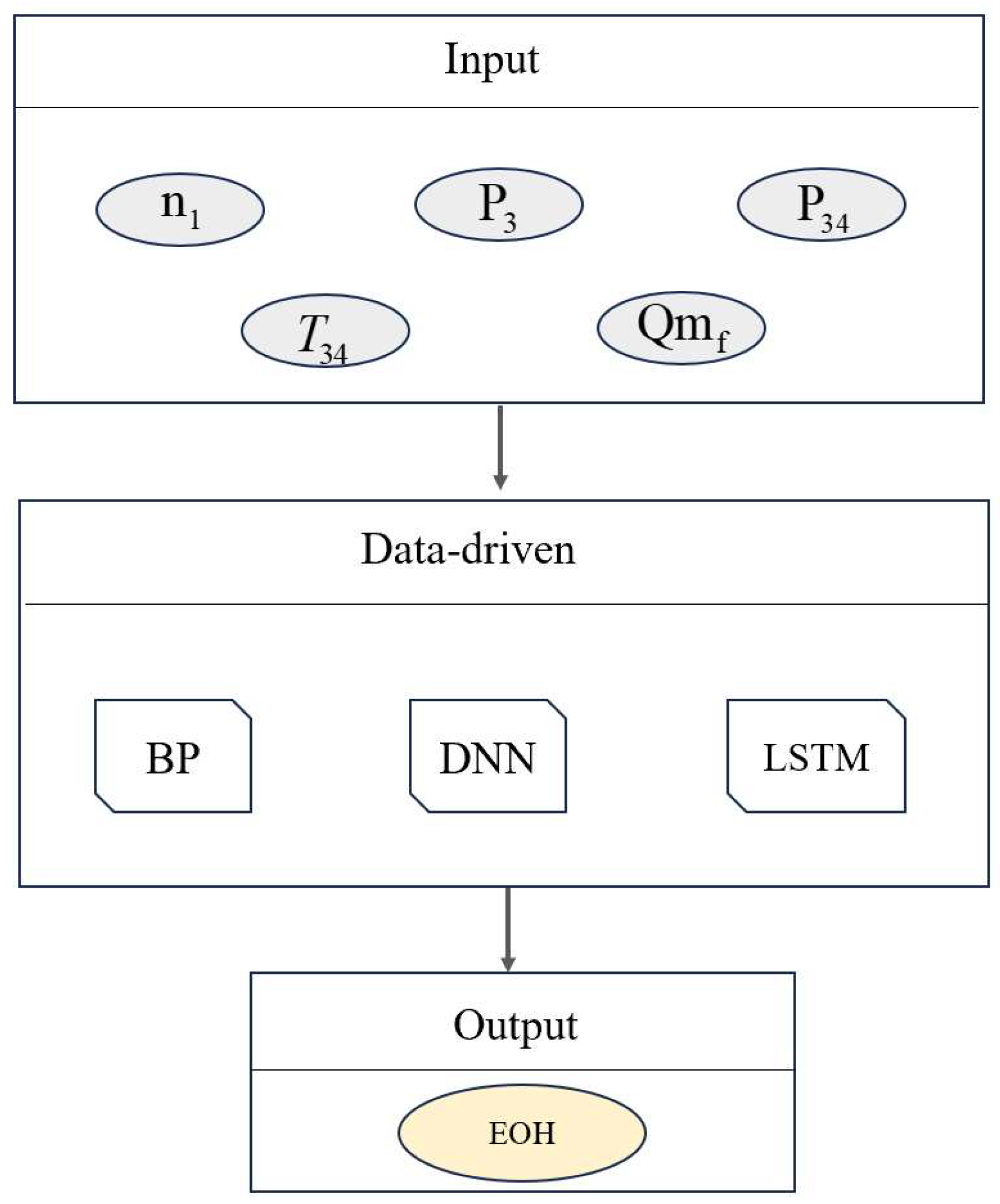
2.4. Surrogate Model Based on the Lifetime Dataset
3. Results and Discussion
3.1. Validation of Lifetime Data Sets
3.1.1. Checkpoint Acquisition for Lifetime Calculation
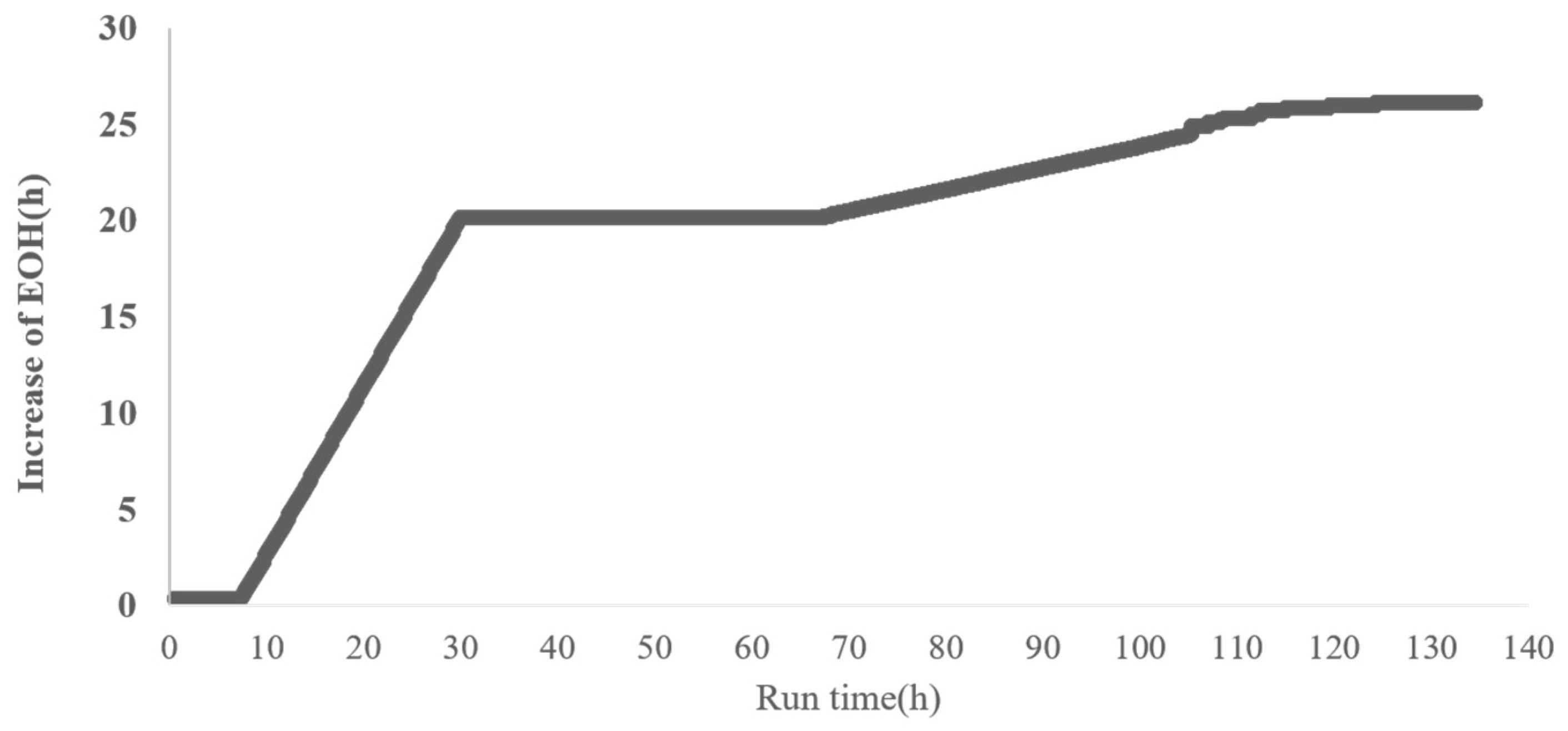
3.1.2. Calculation and Verification of Lifetime
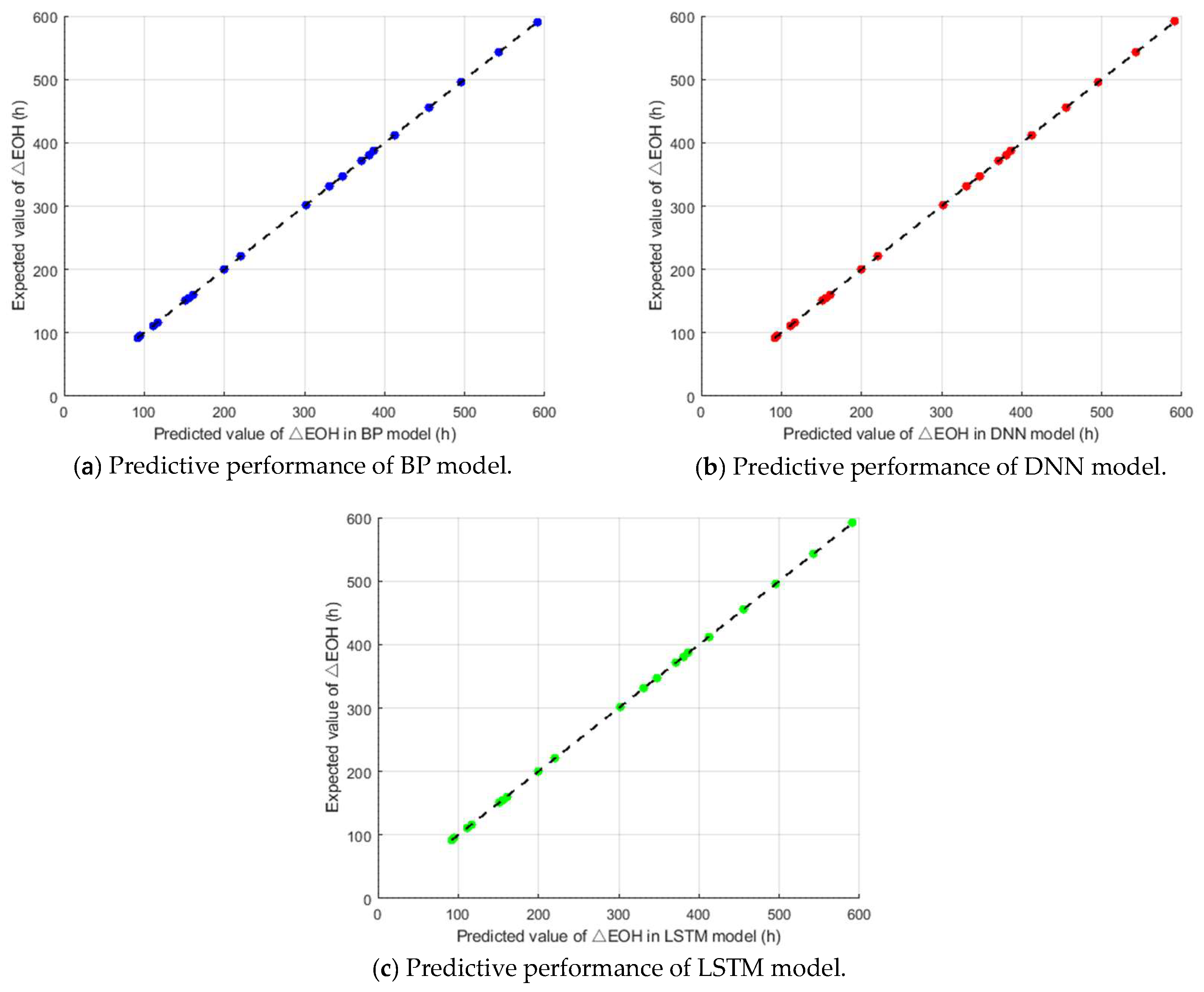
3.2. Prediction Effect of Different Surrogate Models
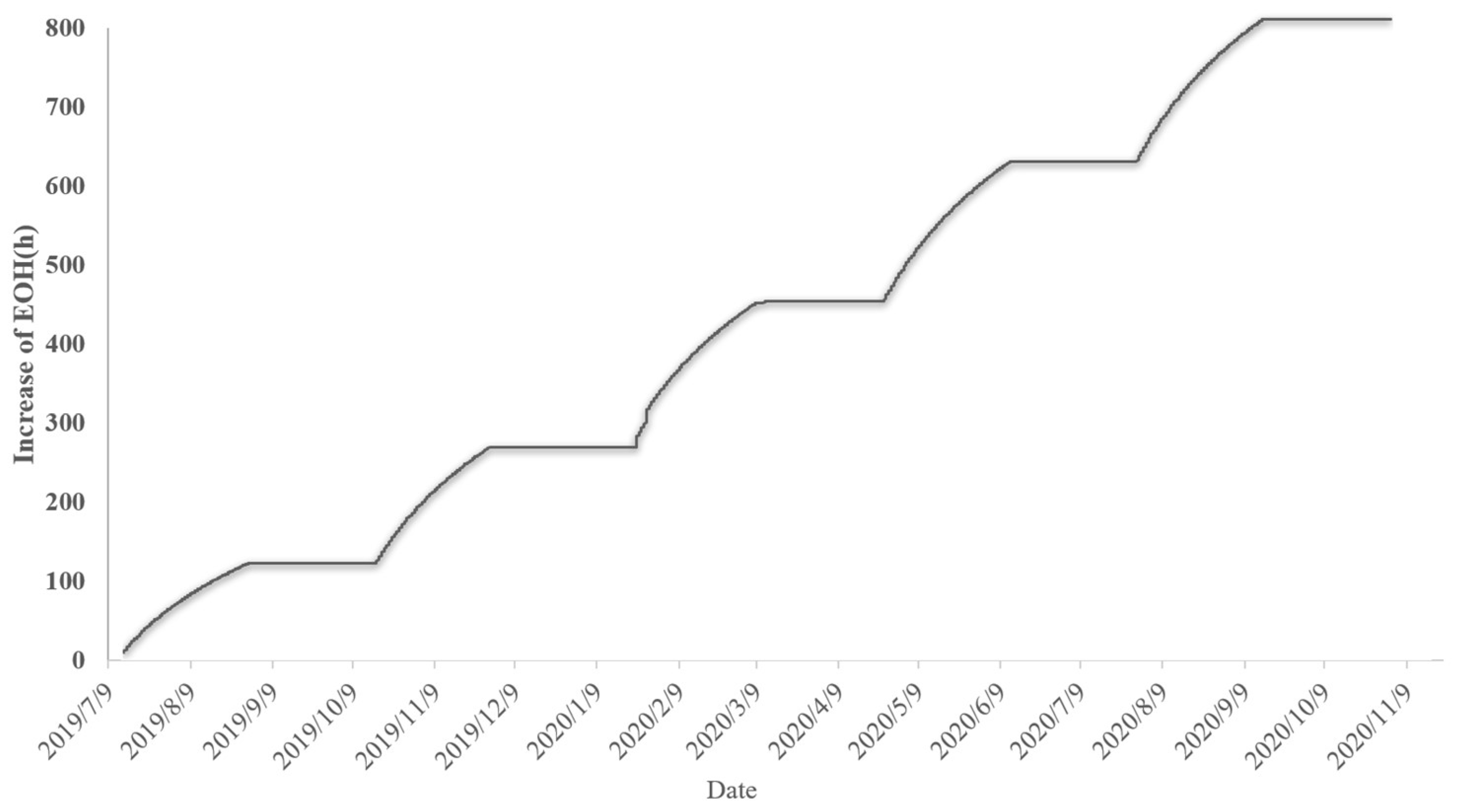
3.3. Application of the Life Prediction Method
4. Conclusions
Author Contributions
Funding
Data Availability Statement
Conflicts of Interest
References
- Rajabinezhad, M.; Bahrami, A.; Mousavinia, M.; Seyedi, S.J.; Taheri, P. Corrosion-fatigue failure of gas-turbine blades in an oil and gas production plant. Materials 2020, 13, 900. [Google Scholar] [CrossRef] [PubMed]
- Saturday, E.G.; Li, Y.; Ogiriki, E.; Newby, M. Creep-life usage analysis and tracking for industrial gas turbines. J. Propuls. Power 2017, 33, 1305–1314. [Google Scholar] [CrossRef]
- Zhou, D.; Wei, T.; Zhang, H.; Ma, S.; Weng, S. A damage evaluation model of turbine blade for gas turbine. J. Eng. Gas Turbines Power 2017, 139, 092602. [Google Scholar] [CrossRef]
- Mazur, Z.; Ortega-Quiroz, G.D.; García-Illescas, R. Evaluation of Creep Damage in a Gas Turbine First Stage Blade. In Proceedings of the International Conference on Nuclear Engineering, Anaheim, CA, USA, 30 July–3 August 2012. [Google Scholar]
- Reyhani, M.R.; Alizadeh, M.; Fathi, A.; Khaledi, H. Turbine blade temperature calculation and life estimation-a sensitivity analysis. Propuls. Power Res. 2013, 2, 148–161. [Google Scholar] [CrossRef]
- Vo, D.-T.; Mai, T.-D.; Kim, B.; Jung, J.-S.; Ryu, J. Numerical investigation of crack initiation in high-pressure gas turbine blade subjected to thermal-fluid-mechanical low-cycle fatigue. Int. J. Heat Mass Transf. 2023, 202, 123748. [Google Scholar] [CrossRef]
- Li, Z.; Wen, Z.; Pei, H.; Yue, X.; Wang, P.; Ai, C.; Yue, Z. Creep life prediction for a nickel-based single crystal turbine blade. Mech. Adv. Mater. Struct. 2022, 29, 6039–6052. [Google Scholar] [CrossRef]
- Lu, Z.; Liu, C.; Yue, Z.; Xu, Y. Probabilistic safe analysis of the working life of a powder metallurgical turbine disc. Mater. Sci. Eng. A 2005, 395, 153–159. [Google Scholar] [CrossRef]
- Zhu, S.; Liu, Q.; Lei, Q.; Wang, Q. Probabilistic fatigue life prediction and reliability assessment of a high pressure turbine disc considering load variations. Int. J. Damage Mech. 2018, 27, 1569–1588. [Google Scholar] [CrossRef]
- Goel, N.; Kumar, A.; Narasimhan, V.; Nayak, A.; Srivastava, A. Health risk assessment and prognosis of gas turbine blades by simulation and statistical methods. In Proceedings of the 2008 Canadian Conference on Electrical and Computer Engineering, Niagara Falls, ON, Canada, 4–7 May 2008. [Google Scholar]
- Voigt, M.; Mücke, R.; Vogeler, K.; Oevermann, M. Probabilistic lifetime analysis for turbine blades based on a combined direct monte carlo and response surface approach. In Proceedings of the ASME 2004 Turbo Expo Conference, Vienna, Austria, 14–17 June 2004. [Google Scholar]
- Song, L.-K.; Bai, G.-C.; Fei, C.-W. Dynamic surrogate modeling approach for probabilistic creep-fatigue life evaluation of turbine disks. Aerosp. Sci. Technol. 2019, 95, 105439. [Google Scholar] [CrossRef]
- Giesecke, D.; Wehking, M.; Friedrichs, J.; Binner, M. A Method for Forecasting the Condition of Several HPT Parts by Using Bayesian Belief Networks. In Proceedings of the ASME 2015 Turbo Expo Conference, Montreal, QC, Canada, 15–19 June 2015. [Google Scholar]
- Sanaye, S.; Hosseini, S. Prediction of blade life cycle for an industrial gas turbine at off-design conditions by applying thermodynamics, turbo-machinery and artificial neural network models. Energy Rep. 2020, 6, 1268–1285. [Google Scholar] [CrossRef]
- Xiong, J.; Zhou, J.; Ma, Y.; Zhang, F.; Lin, C. Adaptive deep learning-based remaining useful life prediction framework for systems with multiple failure patterns. Reliab. Eng. Syst. Saf. 2023, 235, 109244. [Google Scholar] [CrossRef]
- Huang, Y.; Tang, Y.; VanZwieten, J.; Jiang, G.; Ding, T. Remaining useful life estimation of hydrokinetic turbine blades using power signal. In Proceedings of the 2019 IEEE Power & Energy Society General Meeting (PESGM), Atlanta, GA, USA, 4–8 August 2019. [Google Scholar]
- Yin, Z.; Xiong, Y. Geometric algorithms for direct integration of reverse engineering and rapidly reconfigurable mold manufacturing. Int. J. Adv. Manuf. Technol. 2011, 56, 721–727. [Google Scholar] [CrossRef]
- Păunoiu, V.; Teodor, V. Geometric reconfiguration of the multipoint forming dies using reverse engineering. Ann. Dunarea de Jos Univ. Galati Fascicle V Technol. Mach. Build. 2009, 27, 415–418. [Google Scholar]
- Quadir, S.E.; Chen, J.; Forte, D.; Asadizanjani, N.; Shahbazmohamadi, S.; Wang, L.; Chandy, J.; Tehranipoor, M. A survey on chip to system reverse engineering. ACM J. Emerg. Technol. Comput. Syst. (JETC) 2016, 13, 1–34. [Google Scholar] [CrossRef]
- Tian, Y.; Wang, X.; Li, J.; Yang, J.; Liu, Y. Rapid Manufacturing of Turbine Blades Based on Reverse Engineering and 3D Printing Technology. In Proceedings of the Chinese Intelligent Systems Conference 2022; Lecture Notes in Electrical Engineering; Springer: Singapore, 2022; Volume 950. [Google Scholar]
- Brandão, P.; Infante, V.; Deus, A. Thermo-mechanical modeling of a high pressure turbine blade of an airplane gas turbine engine. Procedia Struct. Integr. 2016, 1, 189–196. [Google Scholar] [CrossRef]
- Diraco, G.; Siciliano, P.; Leone, A. Remaining Useful Life Prediction from 3D Scan Data with Genetically Optimized Convolutional Neural Networks. Sensors 2021, 21, 6772. [Google Scholar] [CrossRef] [PubMed]
- Badeer, G.H. GE Aeroderivative Gas Turbines-Design and Operating Features; GE Power Systems: Evendale, OH, USA, 2000. [Google Scholar]
- Xu, D.; Wang, Y.; Liu, X.; Chen, B.; Bu, Y. A novel method and modelling technique for determining the initial geometric imperfection of steel members using 3D scanning. Structures 2023, 49, 855–874. [Google Scholar] [CrossRef]
- Zhou, D.; Wei, T.; Huang, D.; Li, Y.; Zhang, H. A gas path fault diagnostic model of gas turbines based on changes of blade profiles. Eng. Fail. Anal. 2020, 109, 104377. [Google Scholar] [CrossRef]
- He, W.; Deng, Q.; He, J.; Gao, T.; Feng, Z. Effects of Jetting Orifice Geometry Parameters and Channel Reynolds Number on Bended Channel Cooling for a Novel Internal Cooling Structure. In Proceedings of the ASME Turbo Expo 2019, Phoenix, AZ, USA, 17–21 June 2019. [Google Scholar]
- Yuan, F.; Zhu, X.C.; Du, C. Experimental measurement and numerical simulation of 3D flow field in rotating film-cooled turbine. Chin. Soc. Electr. Eng. 2008, 28, 82–87. [Google Scholar]
- Masoomi, M.; Mosavi, A. The one-way FSI method based on RANS-FEM for the open water test of a marine propeller at the different loading conditions. J. Mar. Sci. Eng. 2021, 9, 351. [Google Scholar] [CrossRef]
- Manson, S.; Halford, G. Practical implementation of the double linear damage rule and damage curve approach for treating cumulative fatigue damage. Int. J. Fract. 1981, 17, 169–192. [Google Scholar] [CrossRef]
- Coffin, L., Jr. A study of the effects of cyclic thermal stresses on a ductile metal. Trans. Am. Soc. Mech. Eng. 1954, 76, 931–949. [Google Scholar] [CrossRef]
- Socie, D.F.; Morrow, J.; Chen, W.-C. A procedure for estimating the total fatigue life of notched and cracked members. Eng. Fract. Mech. 1979, 11, 851–859. [Google Scholar] [CrossRef]
- Parhizkar, T.; Mosleh, A.; Roshandel, R. Aging based optimal scheduling framework for power plants using equivalent operating hour approach. Appl. Energy 2017, 205, 1345–1363. [Google Scholar] [CrossRef]
- Ziane, K.; Ilinca, A.; Karganroudi, S.S.; Dimitrova, M. Neural Network Optimization Algorithms to Predict Wind Turbine Blade Fatigue Life under Variable Hygrothermal Conditions. Eng 2021, 2, 278–295. [Google Scholar] [CrossRef]
- Wang, J.; Peng, W.; Bao, Y.; Yang, Y.; Chen, C. VHCF evaluation with BP neural network for centrifugal impeller material affected by internal inclusion and GBF region. Eng. Fail. Anal. 2022, 136, 106193. [Google Scholar]
- Muneer, A.; Taib, S.M.; Naseer, S.; Ali, R.F.; Aziz, I.A. Data-Driven Deep Learning-Based Attention Mechanism for Remaining Useful Life Prediction: Case Study Application to Turbofan Engine Analysis. Electronics 2021, 10, 2453. [Google Scholar] [CrossRef]
- Parra, W.J.V. Probabilistic Approach for Fatigue Life Estimation of Wind Turbine Blades Using Deep Neural Network. Ph.D. Dissertation, Normandie Université, Rouen, France, 2020. [Google Scholar]
- Wang, Y.; Zhao, Y.; Wang, Q.; Gu, W.; Deng, W. Remaining Useful Life Prediction for Aero-Engine based on LSTM-HMM1. In Proceedings of the 2021 5th International Conference on Electronic Information Technology and Computer Engineering, Xiamen, China, 22–24 October 2021. [Google Scholar]
- Liu, J.; Lei, F.; Pan, C.; Hu, D.; Zuo, H. Prediction of remaining useful life of multi-stage aero-engine based on clustering and LSTM fusion. Reliab. Eng. Syst. Saf. 2021, 214, 107807. [Google Scholar] [CrossRef]
- Curry, T.; Behbahani, A. Propulsion directorate/control and engine health management (CEHM): Real-time turbofan engine simulation. In Proceedings of the 2004 IEEE Aerospace Conference Proceedings, Big Sky, MT, USA, 6–13 March 2004. [Google Scholar]


| No. | Reason for Check |
|---|---|
| 1 | Equivalent stress value is maximum |
| 2 | Equivalent strain value is maximum |
| 3 | Temperature is maximum |
| 4 | Special geometric features |
| No. | Equivalent Stress | Temperature | Equivalent Strain |
|---|---|---|---|
| Stationary blade | |||
| 1 | 1481.51 MPa | 1033.34 K | 0.006926 |
| 2 | 1300.34 MPa | 1198.93 K | 0.006033 |
| 3 | 800.83 MPa | 900.29 K | 0.005503 |
| Stationary blade | |||
| 4 | 1308.44 MPa | 1220.02 K | 0.009332 |
| 5 | 1376.43 MPa | 1393.42 K | 0.009482 |
| 6 | 1385.02 MPa | 1300.23 K | 0.009744 |
| No. | (rpm) | (kPa) | (kPa) | (kg/s) | (K) | EOH Increments (h) |
|---|---|---|---|---|---|---|
| 1 | 0.047599 | 0.002423 | 0.000000 | 0.123522 | 0.40163 | 0.000000 |
| 2 | 0.000000 | 0.000000 | 0.010254 | 0.714323 | 0.266652 | 0.125527 |
| 3 | 0.646053 | 0.211596 | 0.103201 | 0.761335 | 0.059797 | 0.221033 |
| 4 | 0.667572 | 0.215596 | 0.122717 | 0.855482 | 0.141488 | 0.264292 |
| 5 | 0.667456 | 0.21525 | 0.126121 | 0.118456 | 0.134114 | 0.329359 |
| 6 | 0.969942 | 0.982835 | 0.970026 | 0.488695 | 0.000000 | 0.469595 |
| 7 | 0.907062 | 0.936506 | 0.91264 | 0.114499 | 0.377102 | 0.487253 |
| 8 | 0.927423 | 0.900578 | 0.958006 | 0.000000 | 0.67072 | 0.642145 |
| 9 | 0.976506 | 0.905042 | 0.916885 | 0.106072 | 0.706214 | 0.707132 |
| 10 | 1.000000 | 1.000000 | 1.000000 | 1.000000 | 1.000000 | 0.880289 |
| 11 | 0.992645 | 0.990454 | 0.984139 | 0.739875 | 0.897642 | 0.932550 |
| 12 | 0.992288 | 0.988131 | 0.980131 | 0.701384 | 0.884362 | 1.000000 |
| No. | Relative Error | No. | Relative Error |
|---|---|---|---|
| 1 | 0.687% | 7 | 0.887% |
| 2 | 0.468% | 8 | 0.746% |
| 3 | 0.446% | 9 | 0.676% |
| 4 | 0.424% | 10 | 0.636% |
| 5 | 0.986% | 11 | 0.543% |
| 6 | 0.894% | 12 | 0.541% |
| Activation Function | Number of Hidden Layers | |
|---|---|---|
| BP | Tansig for the hidden layer, Purelin for the output layer | 9 |
| DNN | ReLU | 3 |
| LSTM | Sigmoid for the input gate and the forget gate, Tanh for the candidate memory cell | 2 |
| Maximum Relative Error | R2 | RMSE | MAE | |
|---|---|---|---|---|
| BP | 0.030% | 0.9601 | 0.1130 | 0.0819 |
| DNN | 0.019% | 0.9734 | 0.0863 | 0.0629 |
| LSTM | 0.014% | 0.9899 | 0.0511 | 0.0372 |
Disclaimer/Publisher’s Note: The statements, opinions and data contained in all publications are solely those of the individual author(s) and contributor(s) and not of MDPI and/or the editor(s). MDPI and/or the editor(s) disclaim responsibility for any injury to people or property resulting from any ideas, methods, instructions or products referred to in the content. |
© 2023 by the authors. Licensee MDPI, Basel, Switzerland. This article is an open access article distributed under the terms and conditions of the Creative Commons Attribution (CC BY) license (https://creativecommons.org/licenses/by/4.0/).
Share and Cite
Xiao, W.; Chen, Y.; Zhang, H.; Shen, D. Remaining Useful Life Prediction Method for High Temperature Blades of Gas Turbines Based on 3D Reconstruction and Machine Learning Techniques. Appl. Sci. 2023, 13, 11079. https://doi.org/10.3390/app131911079
Xiao W, Chen Y, Zhang H, Shen D. Remaining Useful Life Prediction Method for High Temperature Blades of Gas Turbines Based on 3D Reconstruction and Machine Learning Techniques. Applied Sciences. 2023; 13(19):11079. https://doi.org/10.3390/app131911079
Chicago/Turabian StyleXiao, Wang, Yifan Chen, Huisheng Zhang, and Denghai Shen. 2023. "Remaining Useful Life Prediction Method for High Temperature Blades of Gas Turbines Based on 3D Reconstruction and Machine Learning Techniques" Applied Sciences 13, no. 19: 11079. https://doi.org/10.3390/app131911079