

Design of a Low-Energy Earth-Moon Flight Trajectory Using a Planar Auxiliary Problem
Moscow Aviation Institute (MAI), 125080 Moscow, Russia
*
Author to whom correspondence should be addressed.
Appl. Sci. 2023, 13(3), 1967; https://doi.org/10.3390/app13031967
Submission received: 19 December 2022
/
Revised: 28 January 2023
/
Accepted: 30 January 2023
/
Published: 2 February 2023
(This article belongs to the Special Issue Advanced Schemes for Lunar Transfer, Descent and Landing)
Abstract
:The paper presents a sufficiently simple technique for designing a low-energy flight trajectory of a spacecraft (SC) from the Earth to the Moon with insertion into a low circular orbit of the latter. The proposed technique is based on the solution and subsequent analysis of a special model problem, which is a variant of the restricted circular four-body problem (RC4BP) Earth-Sun-SC-Moon; for which it is assumed that the planes of the orbits of all considered bodies coincides. The planar motion of the center of mass of the SC relative to the Earth is considered as perturbed (Sun, Moon). To describe it, equations in osculating elements are used, obtained by using the method of variation of constants based on the analytical solution of the planar circular restricted problem of two bodies (RC2BP)—Earth-SC, for which the rotation of the main axes of the coordinate system (the main plane) is synchronized with the motion of the Sun. The trajectory problem of designing a SC flight from a low circular near-Earth orbit to a low circular selenocentric one (“full” motion model—a restricted four-body problem (R4BP), an ephemeris model) is considered as an optimization one in the impulse formulation. The solution of the main problem is carried out in few (three) stages, on each the appropriate solution of the current variant of the auxiliary problem is determined, which is subsequently used as the basis of the initial approximation to the main one.
1. Introduction
Despite the already quite long and quite solid “history” of the implementation of spacecraft missions to the Moon (both automatic and manned), the ballistic design of SC flight trajectories from low Earth orbit to near-lunar orbits or to the vicinity of the libration points still remains highly non-trivial. This is a direct consequence of the complex and “implicit” essentially non-linear mechanics of motion of the SC center of mass within systems consisting of three or more gravitating bodies. In addition, the generally “weak” controllability of the SC has a significant impact on the design of transfer trajectories (from the standpoint of considering the latter as a controlled dynamical system (i.e., a control object)) since the set of its possible state is extremely small in most cases. Nevertheless, it is known, that a usage of dynamic effects in the framework of the considered complex model of SC motion helps to significantly improve the energy characteristics of the flight trajectory. We are talking here about the possible implementation of the so-called low-energy spacecraft flight trajectories [1,2,3,4,5,6,7,8,9,10] from a low Earth reference orbit to a given selenocentric one. It is quite natural to consider the problem of ballistic design of the trajectory of a low-energy Earth-Moon flight as an optimization problem. However, in itself the formalization of the latter is not so simple, even when using the simplest model of the motion of the SC center of mass. The difficulty here lies in the significant multi-extremality of the problem [1,2,5], due to, firstly, the complex interference and resonant nature of the effects of perturbations from the Moon and the Sun acting on SC trajectory; and secondly, to a very narrow region of admissible states of a SC that satisfy the final conditions in the vicinity of the Moon (entry into a circular orbit of a given radius, etc.). The latter has a particularly strong effect on the convergence of most numerical methods of conditional optimization using the space of local directions. For these reasons, the solution of the problem “directly” turns out to be a very complex and irregular process, overshadowed by significant computational difficulties, and therefore requires consideration of a number of auxiliary problems and analysis of their solutions, due to which a good initial approximation can be found (since the area of convergence of the main problem is too narrow). For the above reasons, the main substantive part of the present work is the description of the approach to finding a solution to the main problem, which is based on the analysis of planar auxiliary problem. Further, in the course of the presentation, their detailed formalization and the method of numerical solution will be presented.
2. Models of Motion
This paper presents a technique for designing a low-energy trajectory for the Earth-Moon flight within the framework of a special planar auxiliary problem. We will consider the motion of the SC center of mass in the framework of the flat RC4BP. Such simplified formulation of the well-known trajectory problem seems appropriate for two reasons: first—the solution obtained for it (numerically) can be used as an initial approximation of the main problem solution (without the considered assumptions). Second, when considering this version of the trajectory problem formulation, it is possible to find out some interesting properties and features from the obtained solution; which are also characterize the main problem. The latter, first of all, include the configuration of celestial bodies—the Earth, the Sun and the Moon, by using which it is possible to build the low-energy trajectory.
In the general case, the motion of the SC center of mass (relative to the Earth along its flight trajectory to the Moon) can be considered within the framework of the restricted four-body problem (R4BP). The latter, as is known, can be described by the following system of ordinary differential equations (undim., see Appendix A):
where r is the radius vector of the SC (vector function of time); ri is the radius vector characterizing the position of the i-th celestial body relative to the gravity center (Earth); Φi—perturbing acceleration from the i-th celestial body. Indexes “E”, “M” and “S” corresponds to the Earth, Moon and Sun. It is important to note that system (1) describes the perturbed motion of the spacecraft’s center of mass precisely in a relative form, not in an absolute one. We will use the same relative form (describing the trajectory motion of the SC) in the course of all subsequent transformations while deriving the equations of motion of the SC.
Further, according to the previously outlined approach to the problem of designing and analyzing low-energy SC trajectories in a simplified model, it is proposed to use next assumptions: trajectories of the SC and celestial bodies—the Moon, the Earth and the Sun—lies in the same plane. The orbits of the Sun and Moon in their relative motion (relative to the Earth) are circular.
Taking into account the assumptions made, it turns out to be convenient to proceed to the description of the plane motion of the SC center of mass in the rotating (“synodic”) coordinate system xCy(z) (see Appendix B), synchronized with the motion of the Sun (see Figure 1). Then the main plane of the system—xCy—is the ecliptic, the main direction (along the x axis) aims to the Sun. In accordance with this, the differential equations of system (1), which describes the motion of the SC, can be rewritten in the form:
or, in a scalar form, taking into account the lowering of the order of the system of differential equations:
where
vectors μμ and ΦS—are perturbing accelerations of the SC (from the side of the Moon and the Sun). According to the accepted assumptions, in the above expressions (3) the value rS, which specifies the position of the Sun, located on the x axis of the uniformly rotating coordinate system xCy(z) is a constant. The absolute angular velocity of the axes rotation for the considered synodic coordinate system xCy(z) can be defined as (relative to the fixed direction of space)
where nS is the mean motion of the Earth relative to the Sun (and the Sun relative to the Earth, respectively); k0 is the unit vector of the coordinate system xCy(z), orthogonal to the main plane (i.e., the plane of motion).
The model of the perturbed motion of the SC, described by relations (2), (2a), and (3) can be further simplified taking into account that the average distance between the SC center of mass and the Earth during its trajectory motion is at least two order smaller to the distance between the Earth and the Sun (rS). This assumption is quite justified in view of the fact, as is known, a low-energy transfer trajectory to the Moon lies within the Earth’s sphere of influence, and can only approach the boundary of it (however, like any other transfer trajectory to the Moon with a possible practical implementation). Then, assuming that
The perturbing acceleration vector of the SC from the side of the Sun can be finally represented as follows
Thus, relations (2) and (2a)–(4) completely describe the perturbed motion of the SC center of mass in a flat restricted circular four-body problem.
Next, we will consider the perturbed motion of the SC center of mass in the accepted model on a basis of the unperturbed motion model corresponding to the restricted problem of two bodies: Earth and SC. The corresponding motion equations (according to the accepted model):
It is easy to show that the restricted circular two-body problem (RC2BP) described by the system of differential Equation (5) naturally has a complete set of “standard” first mechanical integrals: energy h, specific angular momentum σ, and Laplace (Λξ, Λη). Let’s write them down:
The matrix A(t) is defined as follows
In the above expressions (6), the indices ξ and η corresponds to the fixed directions of the coordinate system (CS) axes in inertial space. It is interesting to note that for a system (5) there is one more “atypical” (within the framework of the R2BP) first mechanical integral, which is an analogue of the Jacobi integral from the restricted circular three-body problem (RC3BP)
Equation (7) determines an interesting relationship between the energy and σ constants in a planar circular problem. We also should note here that, according to the accepted model of the perturbed motion of the SC (Equations (2)–(4)) it would not be difficult to describe the SC motion under the framework of the RC3BP Earth-Sun-SC. To do this, in Equation (2a) it suffices to let
In this case (RC3BP), the Jacobi integral is quite naturally present. It takes the form
Further, according to the proposed approach of studying the perturbed SC motion in RC4BP (2)–(4) on a basis of RC2BP (5), it is proposed to use the method of “variation of constants” by Joseph Lagrange [11]. As applied to the system of differential Equation (2a) and the set of the first integrals (6) for system (5), the corresponding equation of the method of variations can be represented as:
where
The perturbation vector (according to equations of the form (2a)):
Scalar expressions φj (x, C) = 0 included in (9) are the first integrals (6) of system (5). By solving system (9) with respect to derivatives
Thus we can obtain differential equations describing the variation of the corresponding components of the vector C:
In the expressions (10), the first differential equation (undim.) (vector form) describes the change in the components of the Laplace vector over time; the second (scalar) is the module of the σ vector. The obtained relations (10) are essentially analogues of the equations in osculating elements, however, they are obtained for the system of differential Equation (5) describing the RC2BP. In this case, the use of a rotating coordinate system makes it possible to simplify the form of the right-hand sides of Equation (9), and obtain a much more useful form of representation for perturbations.
Next, we introduce the following notation
In the above expressions: polar angle β is the angle between the current radius vector of the SC and the main direction of the rotating coordinate system xCy(z) and angle αМ(t) characterizes the current position of the Moon relative to the main direction too. In our assumptions, the Moon’s orbit is assumed to be circular with a dimensionless radius rM equal to 1 (the problem is unidimensionalized as follows: the value of the semi-major axis of the Moon’s orbit equal to 384,400 km is taken as the unit of distance, and the inverse of the mean motion (for this orbit) is taken as the unit of time). The use of dimensionless variables makes it possible to use the well-known relations of the two-body problem in a simple way. So, for example, for the components of the Laplace vector, the following relations are valid, they determine the so-called “eccentricity vector”:
For σ integral
etc., using the obtained Equation (10) and referring to the known relations of the two-body problem:
as well as expressions describing (by means of relations (11)) the components of relative velocities (vx, vy) included in the right-hand sides of system (10):
We can finally obtain a system of differential equations describing the perturbed motion of the spacecraft (in dimensionless form):
The last equation in (13) determines the dependence of the change in the polar angle αM, which characterizes the current position of the Moon relative to the current direction to the Sun. The value nM is the mean motion of the Moon (undim.) which can be defined as:
The components of the perturbing acceleration vectors from the side of the Moon and the Sun can be written as:
Thus, the system of relations (11)–(14) obtained by applying the method of constant variation (9) to integrals (6) will be used to describe the perturbed motion in the planar circular problem of four bodies in order to solve the problem of ballistic design of the Earth-Moon low-energy flight trajectory. The resulting system (11)–(14) is quite cumbersome, but at the same time, it has a number of obvious advantages compared to other ways for describing the SC motion. As will be shown below, these primarily include the convenience of formalizing the optimization problem and the choice of its unknown parameters. We also note that among the advantages, the stability of the numerical integration of system (13)–(14) stands out especially clearly, which generally has a positive effect on the overall computational stability of the process of numerically solving the optimization problem.
3. Optimization Problem Statement
Let us start with the formulation of the main problem. It is required to design a low-energy trajectory of the SC flight from the Earth to the Moon with insertion to a selenacentric low circular orbit of a given height; and at the same time, the total energy costs (total characteristic velocity of a SC) for the flight should minimized. We assume that the impulse approximation is used to describe the active thrust arcs of the motion of the center of mass of the SC. As a motion model, we consider a RC4BP, described by a system (11)–(14). From the mechanical “essence” of the problem, it is obvious that the Sun and the Moon have a significant influence on the trajectory motion of the SC. Especially this concerns to the influence of Sun. Therefore, the design of a low-energy trajectory directly relies on the active usage of lunisolar perturbations. Their influence should help to reduce the total characteristic velocity of the trajectory. The ideal (and well-known) variant of the solution consist of only two impulses to be applied—the initial one from the low Earth reference orbit, and the final one, at the moment when SC inserts the required selenocentric orbit with given parameters. Everything else depends on using the influence of Sun and Moon. Therefore, as a functional (criterion) of the main problem, we consider the total characteristic velocity of SC which is needed for a flight; consider it as a sum of two corresponding impulses. Then the objective functional of the main problem we can write in the following (rather general) form:
Let the vector y consist of unknown parameters of the problem, until we set them explicitly. Its composition will be determined in the future, in the course of the formation and formalization of a sequence of auxiliary problems. Naturally, it is assumed that the functional in expression (15)
where Q is the set of values of parameters y which are admissible under constraints. The latter is formed by the corresponding system, consisting of equalities and inequalities:
Here the functions g and h are also assumed to be continuous and continuously differentiated. As an example, one can explicitly write down a constraint that describes the condition for entering a given selenocentric circular orbit at the end of the flight (this moment of time obviously coincides with the moment of application of the second (last impulse) impulse, inserting the SC to a circular orbit). Within the framework of the planar problem, only its altitude determines the terminal orbit. Therefore, next equality type constraint must be satisfied:
In the above expression (16) RMoon is the radius of the Moon, it is taken equal to 1738 km; hMoon, the altitude of the final circular orbit assumed to be 100 km. Thus, the optimization problem corresponding to the main problem can be formulated (in a “minimal form”) as the following non-linear programming (NLP) problem:
Those, at least, it is required to minimize the functional (15) taking into account the constraint (16). Such a “minimalistic” formulation of the optimization problem turns out to be too general and multivariant, the corresponding problem has a huge number of local minima. Moreover, it is not very obvious, for example, how to set additional restrictions in the framework of statement (17) that would make it possible to relate the positive effects of the influence of lunisolar perturbations, which are determined primarily by the configurations of celestial bodies. Many papers present various approaches and techniques for assessing the influence of the latter [1,2,3,4], but there may be no rigorous constructions or formalization in the form of a finite set of additional restrictions for problem (17), with very rare exceptions. Therefore, in this paper, we propose a step-by-step approach to solving the main problem, in which the emphasis is on maximizing some positive effect of the influence of lunisolar perturbations (mainly solar) on the flight trajectory. Its essence is as follows. Based on the study of works on this problem [1,2,3,4,5,6,7,8,9,10], it is not difficult to draw the following conclusion: a low-energy trajectory is characterized by monotonical increasing of the perigee of the osculating orbit of the SC to a value that exceeds the radius of the Moon’s orbit. The main role here is played by the Sun; the SC trajectory belongs to the outer region (relative to the Moon’s orbit). Let us try to figure this out. Based on the analysis of works on the subject of low-energy trajectories [1,2,5,6] and the assessment of the influence of the Sun, we can draw the following conclusion. The departure impulse transfers the SC to a highly elliptical orbit, the apogee of which is far from the Earth—while providing the required and long-term effect of solar perturbations (with the proper location of the Sun, of course), in which the perigee radius of the orbit increases. Otherwise, reaching the vicinity of the Moon as a whole would be very problematic, or would be realized with too large a difference in velocities. In general, the very fact of reaching the Moon in the vicinity of the perigee of the transfer orbit is understandable, since in this case, the general scheme of the flight resembles a three-impulse one, with the only difference that the second impulse is “realized” by the influence of the Sun. In order to ensure passive gravitational capture of the SC by the Moon at the moment when SC passes the vicinity of the perigee of the transfer orbit, it is clear that it is necessary to minimize the modulus of their relative velocity, so the value of the latter must be greater than the radius of the Moon’s orbit. Therefore, when designing a low-energy trajectory by considering an auxiliary problem, it seems appropriate to consider as an optimality criterion not the sum of impulses (15), but the value of the perigee radius of the transfer orbit when SC approaches the Moon. Obviously, the latter must be maximized. Thus, the question of introducing additional conditions into the problem (17), formalizing the effective usage of the influence of lunisolar perturbations, can be removed. Since, based on simple logic, along the flight path of the SC the influence of the Sun will be the most effective. Another question arises with the “mechanism” of reaching the SC the vicinity of the Moon and its further insertion to the terminal selenocentric orbit. As is known, the dynamical gravity sphere of the Moon itself is relatively small, and on the general scale of the flight trajectory it is a very small area. The size of the latter is known; the entrance to it from the side of the outer region with respect to the Moon’s orbit can be carried out only through the neck in the vicinity of the L2 point of the Earth-Moon system. In this case, it is assumed that, generally speaking, the size of the “inlet neck” is relatively small; otherwise, the selenocentric energy of the SC would be too high, and it would hardly be possible to carry out a passive gravitational capture of the SC by the Moon into a selenocentric elliptical orbit. These reasonings are confirmed by the analysis of Hill surfaces constructed for the derived solutions. The latter will be given in the course of further presentation. Thus, at the current stage of consideration of the auxiliary problem, it seems appropriate to use the condition that ensures that the SC enters some neighborhood of the libration point L2. We formalize this condition in the form of the following inequality-type constraint, which must be satisfied at some time moment t1:
In the above expression, (undim., as a unit of length here and everywhere later 384,400 km is used)—the modulus of the radius vector plotted along the current direction of the Earth-Moon axis and characterizing the position of the center of some neighborhood of the libration point L2. As can be seen from the second relation in (18), the value of the latter is determined by setting the parameter , and when its value is equal to 1, it exactly coincides with the position of the libration point. The value specifies the radius of the neighborhood of the point L2 in which the SC should be at the time t1. In expression (18), the position of the libration point is determined by the value of the corresponding coordinate (undim.), counted from the center of mass of the Moon. The latter is taken equal to . Now, in full accordance with the above reasoning, let us finally formulate an auxiliary problem of trajectory optimization of the first stage: we will solve the problem of designing the spacecraft’s transfer trajectory from the Earth’s low circular reference orbit up to a given neighborhood of the libration point L2. In this case, the radius of the perigee of the transfer orbit when SC reaches the designated neighborhood is considered as criterion. The latter obviously needs to be maximized. Let us formalize the optimization problem of the first stage. The target functional is defined as:
and as the only constraint of the inequality type here we use relation (18).
The vector of unknown parameters y of the problem:
In the above expression (20): β0 is the polar angle characterizing the position of the SC at the moment of its launch from a low Earth reference circular orbit (altitude 200 km); it is started to counting from the current direction to the Sun (at the time of launch!). It is important to note that the departure impulse is applied at the point of the circular orbit corresponding to the perigee of the transfer orbit at the time when mission starts, therefore, the initial position of the apsidal line of the transfer orbit is determined by the same angle; —initial value of the apogee radius (undim.) of the transfer orbit; —polar angle characterizing the position of the Moon at start; counted from the current direction to the Sun; t1 is the moment of time (undim.) of reaching a given neighborhood of the point L2. At the current stage of solving the problem of designing a low-energy flight trajectory (17), the motion of the center of mass of the SC is considered on a closed time interval. Finally, the auxiliary trajectory problem of the first stage of the form (18)–(20) can be represented in the following form:
In this case, the vector of parameters
(specifying the neighborhood of the libration points) is selected manually during the process of solving an auxiliary problem. More details about the choice of the values of the latter will be discussed in the course of further presentation.
By remembering that reaching a given neighborhood of the libration point L2 by SC is not a complete solution to the problem of designing low-energy trajectory (with access to a given low circular selenocentric orbit), now we proceed to the formulation and further formalization of the trajectory optimization problem of the second stage:
It is required to design a low-energy trajectory of the SC, starting from a low circular orbit of the Earth and up to reaching a given selenocentric orbit. As an optimality criterion, the radius of the perigee of the transfer orbit is still considered (should be maximized). It is assumed that the vehicle’s trajectory still passes through the vicinity of the libration point L2 (considered at the previous stage of solving the main problem), while the coefficients of the form (22) can be slightly corrected. Taking into account the assumptions have made, the problem of the second stage can be represented as:
In the above expressions (23), the second condition of the equality type (among the conditions that form the set Q) meets the requirement that the SC reach a given position (RMoon + hMoon) relative to the Moon at time . Thus, an equality type constraint of the form (16) has been added to the optimization problem of the second stage; this is the main difference between the latter and problem (21). At the same time, the dimension of the vector y also increased in a proper way: the time increment Δtf was added to its components; during Δtf the SC performs a passive motion from a certain point in the vicinity of L2 (reached at time t1) to a circular selenacentric orbit.
Before we continue with the third stage problem, it should be mentioned here that the final state vector components of the SC (relative to the Moon) and the corresponding value of the braking impulse ΔVf within the considered model of motion could be determined as follows:
Now we proceed to the formulation of the problem of the third (and final) stage: it is required to design a low-energy trajectory of the spacecraft’s center of mass, starting from a low circular orbit of the Earth and reaching a given selenocentric orbit. As an optimality criterion, the total characteristic velocity of the flight is considered, which is determined as the sum of the departure impulse near the Earth and the braking impulse near the Moon. It is assumed that the vehicle’s trajectory still passes through the vicinity of the libration point L2 (considered at the previous stages of solving the main problem). The above formulation generally corresponds to a problem of the form (17). The functional of the third stage problem can be represented as:
where the magnitude of the initial (departure) velocity impulse ΔV0 can be determined as
and the value of ΔVf is given by expression (24). Then finally, the optimization problem of the third stage can be formalized as follows:
Finally, let us summarized the main aspects of the given 3-stage algorithm for solving a flat auxiliary problem in a form of a simple scheme (with some additional comments) (see Box 1):
Box 1. 3-stage algorithm for solving a flat auxiliary problem.
- Solving a first-stage problem (see (21)):minimize (19) by varying vector (20), taking into account inequality type constraint in (21); this stage is the simplest one and problem (21) can be solved by using any variant of quasinewtonian algorithm; the set of a parameters (22) should be chosen from some admissible diapason, we can recommend here
- Solving a second-stage problem (see (23)):once again it is necessary to find a constraint minimum of functional (19), but this time by varying vectorand taking into account an equality type constraint which corresponds to a required value of a given radius of final selenacentric orbit; the inequality type constraint from a previous stage also should be used here. To find a numerical solution in that case it is assumed to use a solution of a first stage problem that was derived previously. Adding the equality constraint makes this problem very sensitive to variation of any of the unknown parameters, but as it was shown by our own experience in that problem (usage of a graph-analytical approach), small and slightly variations of (22) provides for us an ability to sufficiently easily satisfy altitude constraint and thus, define the value of Δtf. Moreover, for different values of a given altitude of a final orbit it was enough to vary only first coefficient from (22) for a value that not exceeds ±0.02. The variation of first coefficient from (22) provides a direct influence to a value of an axial projection of the SC relative velocity vector in RC3BP Moon-Earth-SC (the direction of an axial projection coincides with the current Moon to Earth direction). Changing of it provides for a SC ability to proceed through the vicinity of L2 libration point inside the Hill sphere and after that approaches to the Moon.
- Solving a third-stage problem (see (25)):this time the sum of two impulsesshould be minimized under the same constraints from the previous second stage problem; the vector of unknowns also is the same. Changing of a criterion does not provide additional complexities in search of a numerical solution (it is interesting by itself). Like previously, as an initial guess was used the solution from the previous (second) stage problem.
Next, the solution that we have obtained from the flat auxiliary problem now can be used as an initial approximation for solving the same problem but in a full model (3-dimensional motion, ICRS (J2000.0) reference system, ephemeris model); as well as solving the problems of designing trajectories to the libration points L1 and L2.
So, let us briefly describe the formulation of the problem of a designing low-energy Earth-to-Moon flight within the framework of a “complete” model of motion. Now, to describe the motion of the SC, as before, the R4BP is used: Earth—SC—Sun—Moon (system (1), ephemeris model (JPL DE421)). The Earth is the central body and as a main reference ICRS (J2000.0) coordinate system is used. The SC starts its motion at some initial time t0 from a low circular geocentric orbit of a given radius r0 and inclination i0. Then performs a flight to the Moon, in the close vicinity of which a braking impulse is realized, inserting a SC to a circular circumlunar orbit of a given altitude hMoon and with a given inclination iMoon (relative to the lunar equator). The initial state of the SC is determined by the following relations:
For the purpose of some regularization of the optimization problem, we can consider a third (second in a row) additional velocity impulse (correction)—the so-called apogee velocity impulse ΔV2, realized along the transfer trajectory at time t1. Then
Why we used another impulse here? Because we have thought that the adding of the third (presumably small) impulse will help SC to reach the required vicinity of L2 point (for a problem with a “full” or “complete model of motion”) with some admissible state. We assumed that this impulse should take place somewhere near the apogee of the SC flight trajectory: also, we thought that by using it we would truncate (if needed) possible trajectory declinations right before the SC reaches the close vicinity of the L2 point. The usage of the additional impulse here somehow resemblance with the usage of the parameters (22) in auxiliary problem—it helps us to derive a required solution in more robust way. Despite the fact that the number of unknowns increased, the numerical stability also got better.
The value of the vector of the final velocity impulse ΔVf (when the SC reaches a given selenocentric orbit) can be determined as follows:
In addition, at the moment tf, the following conditions must be satisfied; they describe the terminal state of the SC (circular selenocentric orbit of a given radius\given altitude):
In the above expressions (28), the third condition corresponds to the restriction on the inclination of the terminal selenocentric orbit, which should be equal to if.
The optimization problem corresponding to the considered trajectory problem of designing a low-energy trajectory can be formalized as the following non-linear programming problem:
The unknown parameters of (29) (components of the vector z): the magnitude of the initial velocity impulse ΔV0; the longitude of the ascending node Ω0, and the argument of latitude u0 of the SC starting point from the low circular geocentric orbit of a given inclination i0; times of launch t0 and SC insertion into a given selenocentric orbit tf; the moment of application of the apogee velocity impulse t1; components of the apogee velocity impulse vector ΔV2.
Now it is understandable that for solving problem (29) we need to know the optimal “nodal” moments of time (t0 and tf), the value of the first impulse, apogee radius (at the moment t0) of the SC transfer orbit, and also the estimation of the relative position between a Laplace vector and direction to the Sun (at the moment of start). All this info we can directly collect from the derived solution of the flat auxiliary problem, and define the required time moments and position of the Laplace vector by analyzing the optimal configuration of the corresponding celestial bodies (by using ephemerid model).
4. Results
The numerical solution of problem (21), a non-linear programming problem with a single inequality-type constraint, can be found very simply and quickly, for example, using any quasi-Newtonian method. In this case, the determination of the initial approximation is not a difficult problem; in general, as practice has shown, the problem is relatively easy to solve even with almost arbitrary assignment of the values of the vector y (with the exception, perhaps, of the duration of the flight). Only the convergence time of the method to the solution will differ. In the numerical solution of the auxiliary problem of the first stage, the values of the components of the parameter vector (22) were, as a rule, chosen from the range
The value of the upper limit of the change of the first parameter at 0.98 is due to the requirement for the presence of a negative radial component of the SC relative velocity vector in the vicinity of the L2 point (with respect to the Moon, of course). Otherwise, the SC either does not enter the Moon’s gravity sphere at all, or does not stay there for a long time, as practice has shown. The range of allowable radius values in the vicinity of the libration point corresponds to values from 1000 km to 20,000 km.
Figure 2, Figure 3, Figure 4, Figure 5, Figure 6, Figure 7, Figure 8, Figure 9, Figure 10, Figure 11, Figure 12, Figure 13, Figure 14 and Figure 15 show the characteristics of the spacecraft’s flight trajectory to a given neighborhood of the point L2, obtained as a result of solving problem (21). Vector of unknown parameters:
according to which the initial value of the polar angle β0 was: −10.539971 degrees, the optimal initial value of the apogee radius of the transfer orbit: 1.138961 million km; the angle characterizing the initial position of the Moon relative to the current direction to the Sun (at the time of launch) was 243.192276 degrees; the duration of the flight turned out to be 94.686633 days. The resulting solution was found for the following values of the coefficients (22) (specifying the neighborhood of the point L2):
It turned out that at the final moment of time the radius vector of the SC belongs to the boundary of the considered region. The value of the perigee radius of the transfer orbit at the moment of the end of the SC motion (criterion) was 1.188564 (undim.), or 456,884.072099 km.
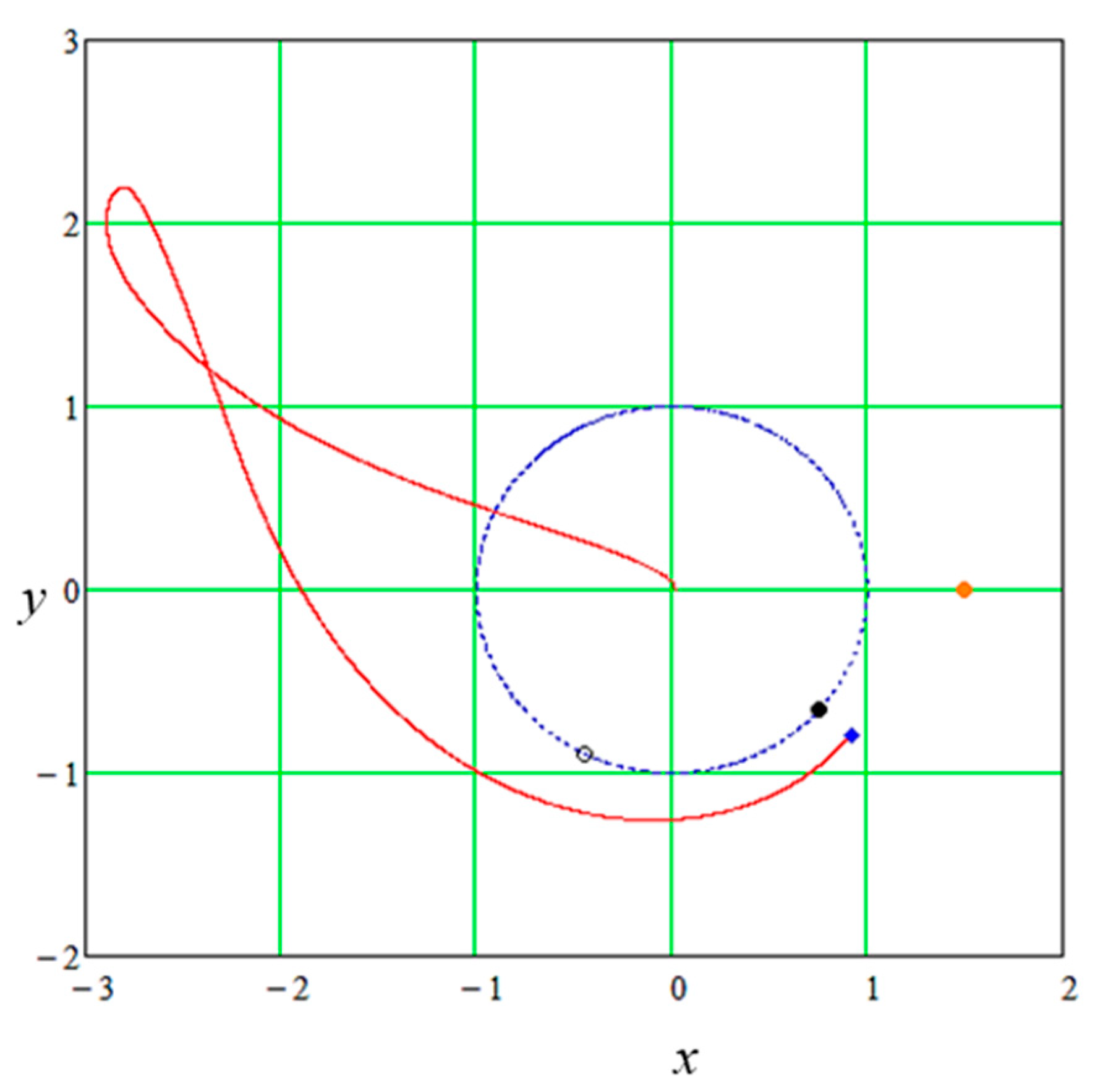
The dependence presented in Figure 4 clearly demonstrates the flight of the spacecraft to the Moon from the outer region with respect to its orbit.
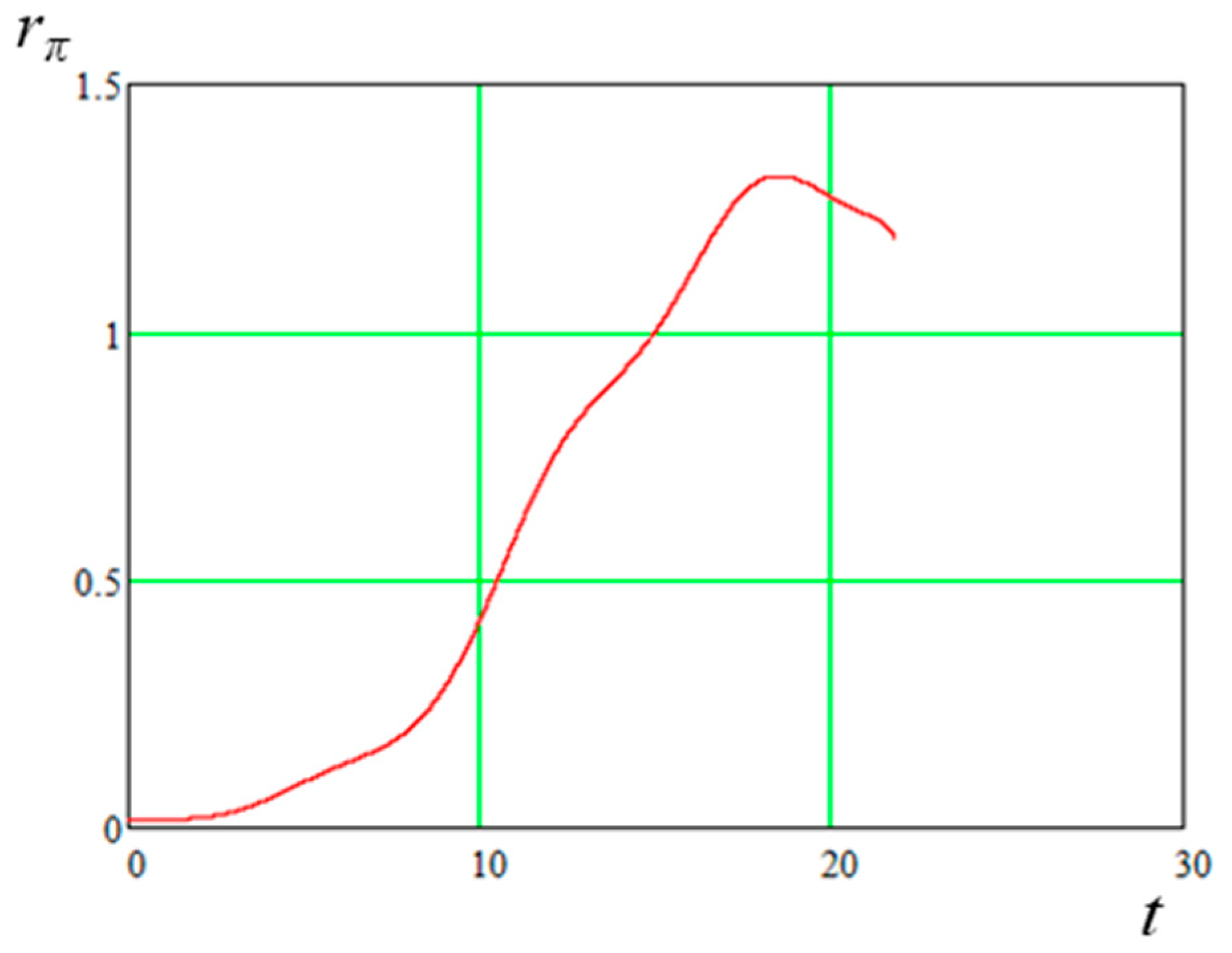
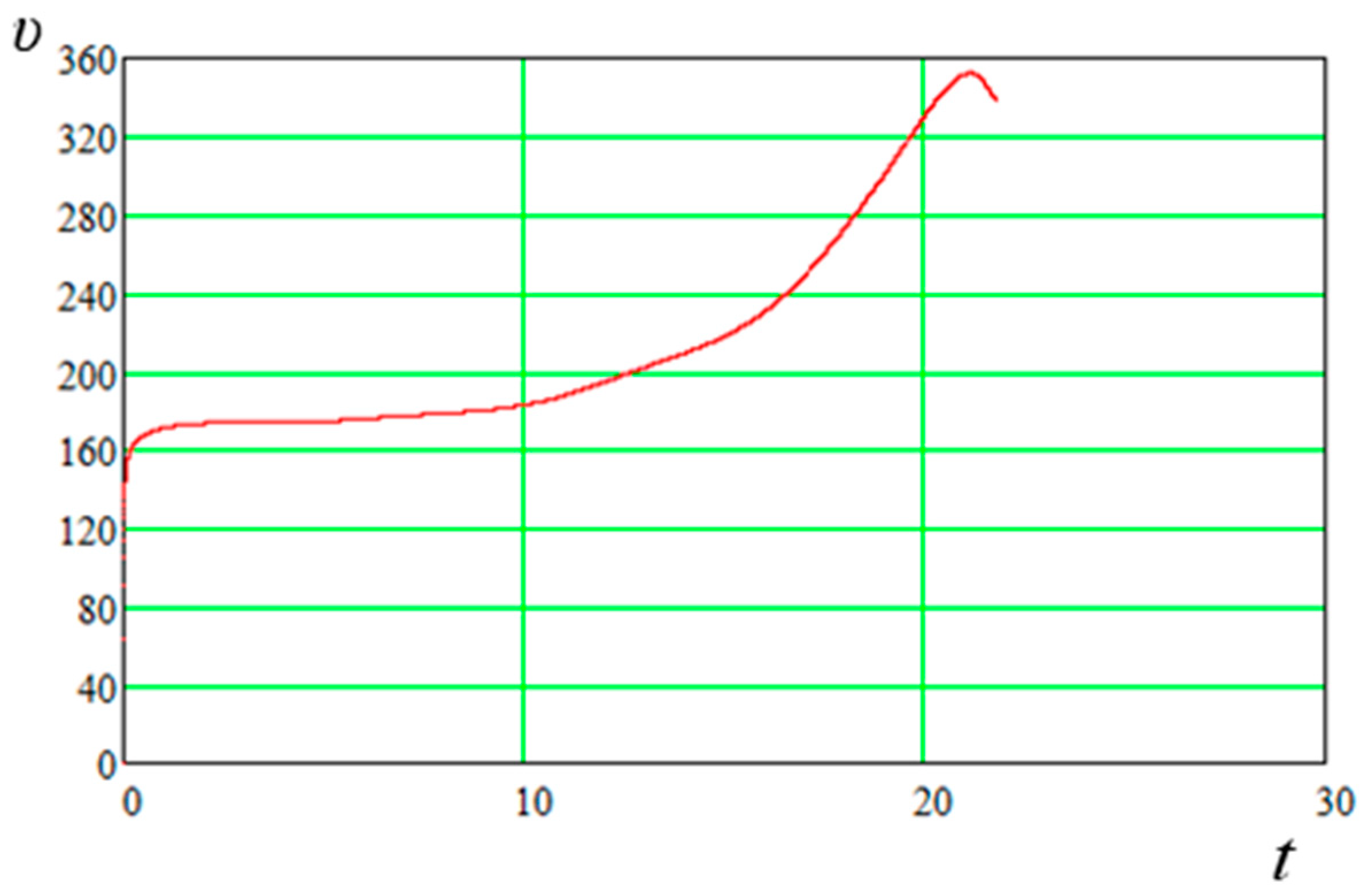
Figure 5 and Figure 6 show the time dependences of changes in the radii of the perigee and apogee of the transfer orbit. One can see an intensive and generally monotonous increase in the perigee radius of the orbit, with the exception of only the last section; the apogee radius varies nonmonotonically, but over a sufficiently large range. The strong influence of the Sun is clearly manifested. Figure 8 shows a monotonous and generally very intense change in the eccentricity in the direction of decreasing the value of the latter. Figure 9 shows a strong short-period perturbation of the semi-major axis of the transfer orbit; it is interesting to note that at the end of the revolution, there is no secular departure of the latter, especially in comparison with other elements; which generally agrees with the estimates of secular shifts of orbital elements under the action of gravitational perturbations from other bodies.
Figure 10 shows a dependence typical of low-energy trajectories plotted on the “eccentricity-major axis” plane; according to which there is an “exchange” of the eccentricity value for the value of the semi-major axis; at the same time, by the end of the transfer orbit, there is practically no secular deviation of the semi-major axis, which cannot be said about the eccentricity.
Figure 12 shows the dependence of the change in the true anomaly of the SC along the flight trajectory. It can be seen that the spacecraft completes about one full orbit at the moment of reaching a given vicinity of the libration point, while the final value of the true anomaly indicates the presence of a negative radial velocity component, which is decisive from the point of view of the possibility of the spacecraft entering the Moon’s gravity sphere through the vicinity of the L2 point.
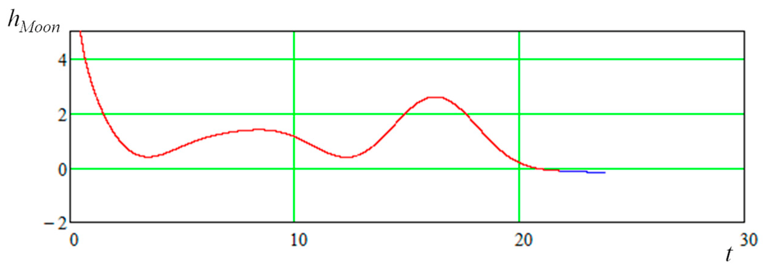
From Figure 14 and Figure 15 it follows that the selenocentric energy constant becomes negative long before the SC enters the Moon’s gravity sphere.
For the numerical solution of the considered optimization problem of the second stage, it is quite natural to use the corresponding solution of the first stage problem as an initial approximation. However, it is important to note here that the addition of a constraint of the form (16) significantly increases the sensitivity of the problem under consideration to variations in its unknown parameters. Thus, the restriction on reaching a given altitude above the surface of the Moon turns out to be quite “rigid”; this is due to the very strong influence of disturbances acting on the trajectory of the selenocentric motion of the SC from the side of the Earth and the Sun, which leads to a very rapid evolution of its orbit. So, for example, when carrying out practical calculations within the framework of the procedure for solving the problem under consideration, even cases of reversal of the selenocentric orbital motion of the SC were recorded. The latter clearly demonstrates how strong perturbations can be. Such effects can adversely affect the stability of numerical integration during SC motion in the vicinity of the Moon and, consequently, the overall stability of the computational process of numerically solving the optimization problem of the second stage. Therefore, it seems appropriate to use the following “graph-analytical approach” to determine the initial approximation for the problem under consideration. It is based, of course, on the solution of the problem of the first stage. It mainly allows one to determine the approximation to the parameter Δtf and, if necessary, correct the values of parameters (22) to satisfy the condition of the form (16). The essence of the approach is very simple and is as follows: the optimal trajectory obtained as a result of solving the problem of the first stage is numerically integrated within the framework of the adopted motion model starting from the time t1 (determined at the first stage of the solution) up to the time moment , where the value is set arbitrarily and can up to several tens of days. In this case, the fulfillment of a condition of the form (16) is monitored, i.e., altitude condition (first of all, the possibility of reachability), as well as the value of the final (second) velocity impulse necessary to transfer the SC to a circular selenocentric orbit (it should not be too large (!)). In order to satisfy the latter, it is proposed to vary the parameters (22). As practice has shown, a small change in any one of them is quite sufficient, for example. Naturally, in this case, it is required to solve the problem of the first stage again, which does not present any difficulties at all, especially in view of the presence of a “reference” solution. Next, consider an example of solving the problem of the second stage using the described approach. So, let’s set the value equal to 30 days and numerically integrate the second part of the trajectory, starting from the moment t1 = 21.804723 undim. (94.686633 days) and ending with the moment of time equal to 28.713213 undim. (124.686633 days). As a result, we obtain the trajectory of the spacecraft’s center of mass, presented together with its characteristics in Figure 16, Figure 17, Figure 18, Figure 19, Figure 20, Figure 21, Figure 22 and Figure 23.
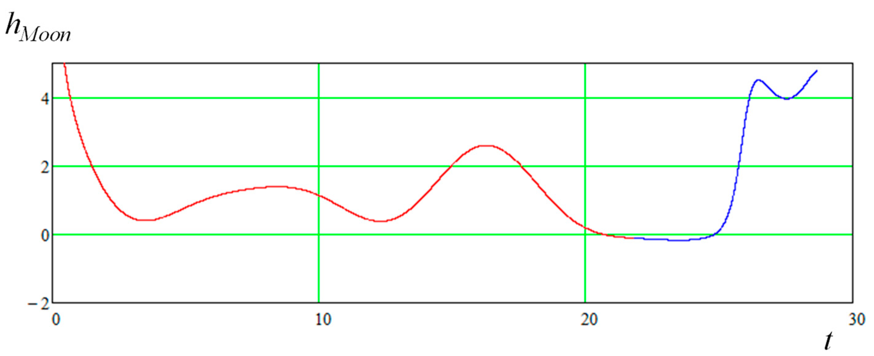
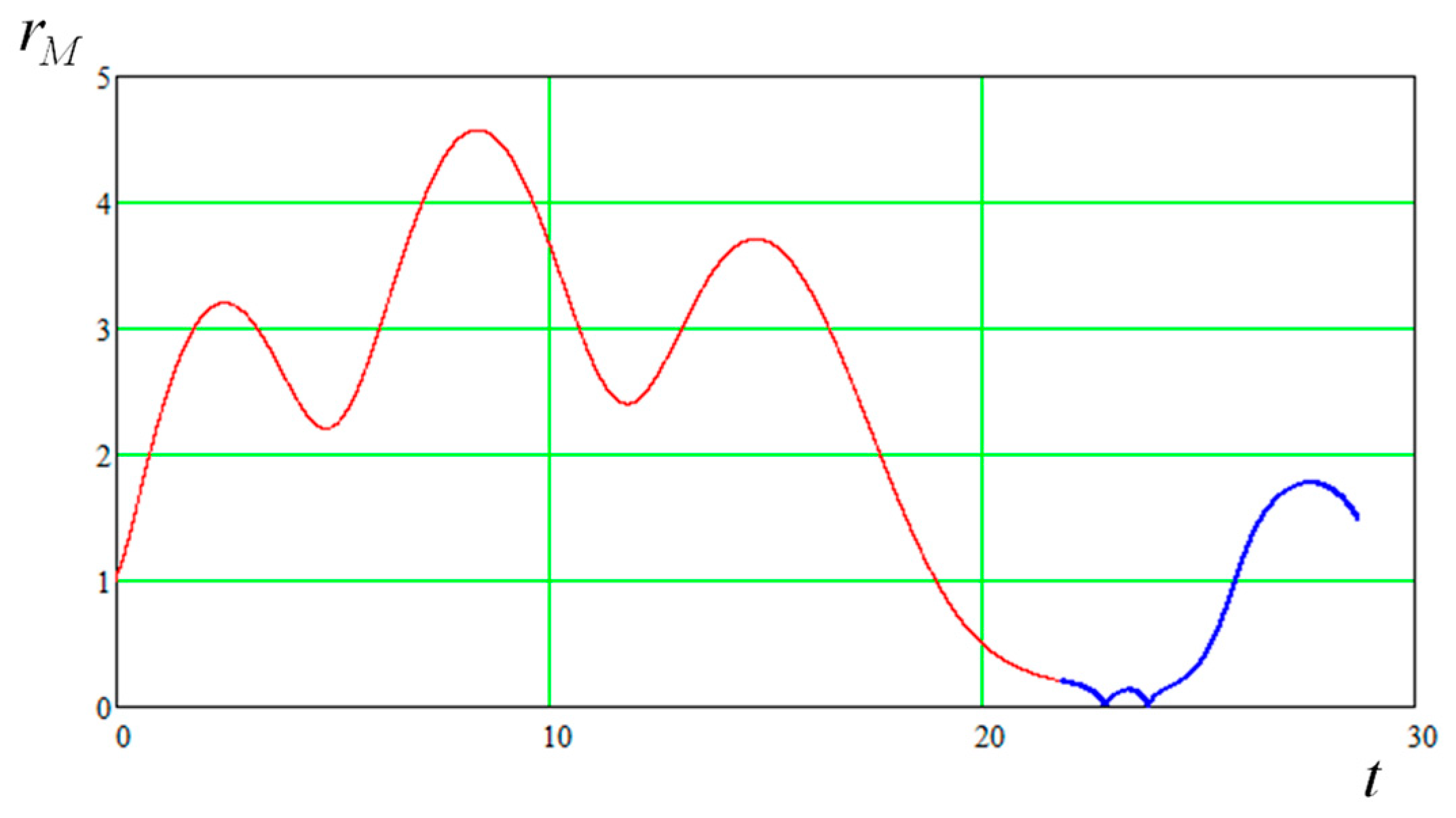
In Figure 17 and Figure 18, the solid black line represents the trajectory of the spacecraft’s center of mass, starting from the movement in the vicinity of the libration point (t1) and up to leaving the Moon’s gravity sphere (). The SC in its motion passes into the gravisphere (Hill’s sphere) of the Moon through the “throat” from the point L2, then makes almost two turns in a closed selenocentric orbit (see Figure 19, Figure 20, Figure 21 and Figure 22). The Sun leaves the sphere of influence of the Moon through the neck of point L1. Here, for us, the section of the selenocentric movement of the SC is of the greatest interest. Let’s explore it. To verify the fulfillment of a condition of the form (16), we plot the dependence of the selenocentric distance along the transfer trajectory. The latter is shown in Figure 24.
The presented figure clearly shows two close successive approaches to the Moon, which quite naturally fall on the area of the “circumlunar” motion of the spacecraft (blue curve). It is clear that both of these approaches correspond to passages of the periapsis of the osculating elliptical selenocentric orbit. First of all, it is required to estimate the height of these passages. Therefore, we construct a dependence that describes the change in the relative distance between the radius vector of the SC center of mass and the circular selenocentric orbit of a given altitude during its movement along the circumlunar part of the trajectory. Obviously, the corresponding dependence directly reflects a condition of the form (16). It is shown in Figure 25.
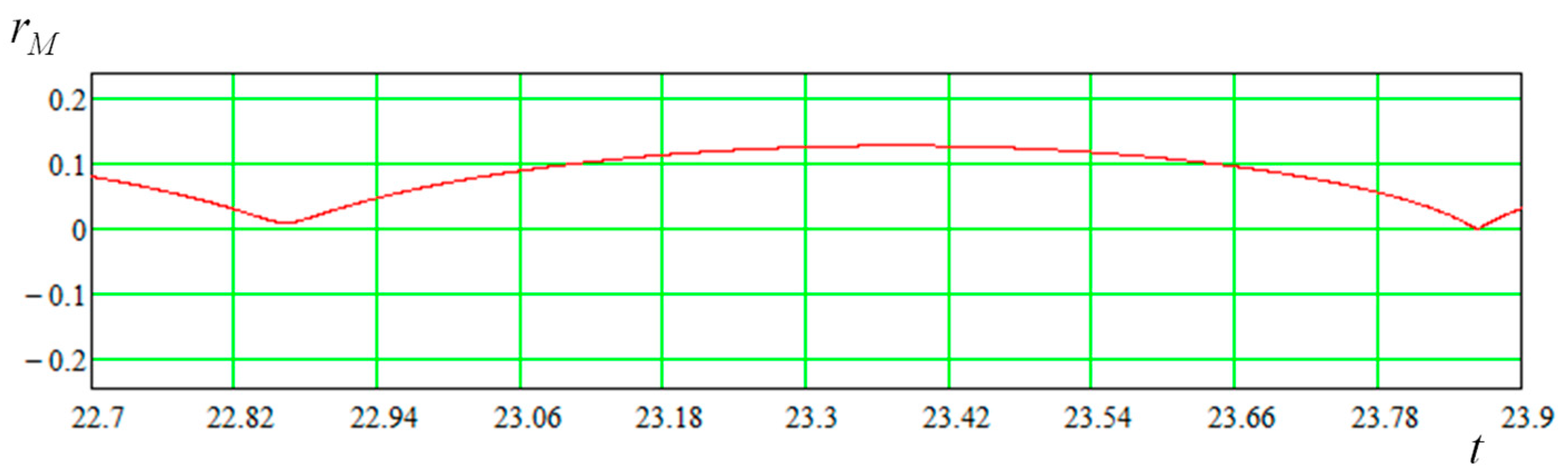
For the presented dependence, we are primarily interested in the range of the argument t—dimensionless time—for which the sign of the relative distance changes. Because On the boundaries of the such regions, there are points of intersection between the selenocentric trajectory of the SC with and final circular orbit. In the possible limit case, for each region, this can be only one single point, at which, obviously, the periselenium of the elliptical orbit of the SC will be equal to the radius of the terminal circular one. If there are no intersections, or the orbit does not close, it is proposed to slightly change one of the parameters of the form (22), i.e., actually change the conditions for the SC to enter the “throat” in the vicinity of the point L2, and again integrate the trajectory by constructing dependencies of the form 17–26. As mentioned earlier, the latter requires the definition of a new solution to the optimization problem of the first stage, which does not cause any problems at all. Now let’s turn again to dependence type 25 and its enlarged fragment, shown in Figure 26. It can be seen that only during the second close approach, the selenocentric orbit crosses the terminal circular one. The points of intersection of the curve (in the considered case there are only two of them) make it possible to determine two possible moments of time for the realization of the braking impulse. The coordinates (i.e., abscissas) of these points make it possible to determine the initial approximation for the unknown parameter Δtf. The value of the latter can obviously be obtained by considering the difference between the corresponding value of the intersection point coordinate and the value of t1. Any interpolation procedure (for example, conventional linear interpolation) can be used to numerically determine the coordinate of the intersection point. Further, in view of the fact that in our case we obtain two possible values for the parameter Δtf, the final choice of its approximation can be made by comparing the corresponding values of the velocity impulse required to insert the SC to a given circular orbit. In this case, if the estimation of the velocity impulse turns out to be too large (for us it is more than 800 m/s), we again turn to the variation of the parameters of the form (22). As a result, after determining the approximation to the parameter Δtf by using the described graphical-analytical approach, together with the selection (properly) of the coefficients of the form (22), a “pure” solution to the problem of the second stage was obtained. The vector of unknown parameters y in this case was:
It can be seen that the vector of unknown parameters of the problem of the second stage has undergone minor changes compared to the corresponding values of y of the problem of the first stage. The total duration of the flight, counting from the start of the mission from the Earth’s low reference orbit and up to reaching the given selenocentric orbit, is t1 + Δtf = 23.868141 (undim.), which corresponds to 103.646984 days. The value of the braking impulse on the obtained solution: ΔVf = 0.638125 km/s. The problem of the second stage was solved for the following values of the coefficients (22):
For the numerical solution of the third stage problem, the vector of unknown parameters obtained at the previous (second) stage is used as an initial approximation. As a result, for problem (25) the vector y:
The solution to the problem of the third stage was found for the same values of the coefficients (22) that were chosen for the problem of the second stage, i.e.,
It is interesting to note that the position of the spacecraft at time t1, upon reaching a given neighborhood of the point L2, also belongs to its boundary. As a result of solving problem (25), the total characteristic velocity of the flight turned out to be 3.829224 km/s, the value of the departure impulse from the Earth ΔV0 = 3.194456 km/s; the magnitude of the braking impulse near the Moon is ΔVf = 0.634768 km/s. The total duration of the flight was t1 + Δtf = 23.852629 (undim.), which corresponds to 103.579628 days. The initial value of the polar angle β0 was: −10.636105 degrees, the optimal initial value of the apogee radius of the transfer orbit: 1.138830 million km; the angle characterizing the initial position of the Moon relative to the current direction to the Sun (at the time of launch) was 243.886838 degrees. Further, Figure 27, Figure 28, Figure 29, Figure 30 and Figure 31 (all undim.) show the optimal trajectory of a low-energy spacecraft flight obtained by solving problem (25) as well as a number of dependencies characterizing it.
The optimal two-impulse low-energy spacecraft flight trajectory obtained by solving problem (25) is shown in Figure 27. It is clearly seen that the resulting trajectory of problem (25) with a functional expressing the total characteristic velocity of a two-impulse flight almost exactly coincides with the trajectories obtained by solving problems (21) and (23) with a functional (19). This is also confirmed by a direct comparison of the corresponding values of the vector of unknown parameters y for the three considered problems. In general, this indicates the correctness of the approach, in which the perigee radius of the transfer orbit was chosen as the criterion for the optimality of the auxiliary problem; it also once again emphasizes the role of the Sun, because the considered formulations of the trajectory problem are aimed at maximizing the effect of perturbations (mainly from the Sun).
Finally, let us consider the solution of problem (29). The solution of (29) for a given value of the initial inclination i0 = 51.80 (to the geoequator) was found: from the solution of the flat auxiliary problem, approximations to the parameters (ΔV0, t0, tf) and optimal configuration of celestial bodies (Earth—Sun—Moon) were obtained (corresponds to β0, αM0). Next, a numerical solution of the optimization problem was determined—for this, the nonlocal CMA-ES algorithm [12] was used, which is a variant of the evolutionary strategy with adaptation of the covariance matrix. The numerical integration of the equations of motion was carried out using the Dorman and Prince DOPRI853 algorithm [13]. Below the results of the obtained solution (Figure 31 and Table 1) are presented (briefly).
Finally, let us compare the solutions of problems (29) and (25). The corresponding results presented in Table 2.
It is easy to see that the derived results are quite close to each other but the solution of the flat auxiliary problem is better as it was expected.
5. Conclusions
The considered approach based on the use of a flat auxiliary problem, has shown its effectiveness in solving the problem of designing a low-energy trajectory. At the same time, it is important to note that the “another one dimension” of the main problem does not introduce any additional sufficient complexities in a solving process. Because the configuration of celestial bodies that was derived as a solution from planar auxiliary problem, provides at the same time the monotonically changing of declination between SC osculating trajectory and Moon orbital plane and thus with sufficiently high rate of change. Alternatively, we can say that the Sun influence provide a rapid alignment between Moon orbital plane and SC trajectory for an optimal configuration from auxiliary solution. By itself, it is a well-known fact and it can easily be checked in a different works [1,2,5,14].
The main advantage in a proposed approach in comparison with the other works [1,2,3,4,5,6,7,8,9,10] is an ability to reduce complexity of solving main problem, cause all other known approaches offers to directly solve problem like (29) (which is very sensitive and multimodal) with or without any suitable initial guess. The latter is not depends on a form of analytical conditions or constraints that should be used in other approaches. The usage of the auxiliary problem help us to build the admissible initial approach for solving problem (29). Any subproblem from the 3-stage approach can be solved numerically sufficiently easy with any local constraint optimization algorithm. It makes the proposed approach some kind more “engineering”. The auxiliary problem has a greater numerical stability in comparison with other—due to its simplified “nature” of cause, but also, due to usage of the system like (13), whose state vector consists of osculating elements. In addition, for some other problems (4BP) with a possible multirevolutional SC motion around the main body, system (13) can be used in a combined manner with asymptotical technic (numerical or maybe analytical averaging).
Author Contributions
Conceptualization, I.N. and V.S.; methodology, I.N.; software I.N. and V.S.; validation, I.N. and V.S.; formal analysis, I.N.; investigation, I.N. and V.S.; resources, V.S.; data curation, V.S.; writing—original draft preparation, I.N.; writing—review and editing I.N.; visualization, V.S.; supervision, I.N.; project administration, I.N.; funding acquisition, I.N. All authors have read and agreed to the published version of the manuscript.
Funding
This work was supported by the Russian Science Foundation grant no. 22-79-10206, https://rscf.ru/project/22-79-10206/, accessed on 1 August 2022.
Institutional Review Board Statement
Not applicable.
Informed Consent Statement
Not applicable.
Data Availability Statement
Some amount of data is available and can be found here: https://drive.google.com/drive/folders/1JsAXNKrk7BwZ6hFxIkNvQ5OCjQ8JzmRy?usp=sharing, accessed on 1 August 2022.
Conflicts of Interest
The authors declare no conflict of interests.
Appendix A
Almost all variables in a present work are dimensionless. It was provided by using next simple scaling units:
- as unit of length was taken the average value of the semi-major axis of the Moon orbit which assumed to be equal R0 = 384,400 km;
- as unit of time T0 it was taken the inverse value of the mean motion, associated with the geocentric circular orbit with radii equal to R0:where μE = 398,600 km3/s2—is a gravitational parameter of Earth.
Then, accordingly with the proposed definition of length and time units the corresponding units for velocity and acceleration can be expressed as
Appendix B
Coordinate systems
The main coordinate system that used in a present work is a system xCy(z)—geocentric non-inertial, uniformly rotating, basic in terms of describing the SC motion (see Figure 1). The main plane of this system coincides with the ecliptic, the main direction—Cx axis—always aims to the Sun. Its rotation is synchronized with the Sun mean motion (the corresponding angular velocity vector lies on z axis).
ξСη(ζ) coordinate system (see Figure 1)—geocentric non-inertial, non-rotating with the fixed main axises in space. The main plane of this system is also coinciding with ecliptic, main direction—Cξ—coincides with the Sun position at the initial moment of time.
ξMСηM(ζ) coordinate system (see Figure 19)—selenocentric non-inertial. Its main plane and main direction are coinciding with the same ones of the system ξСη(ζ).
xMCyM(zM)—selenocentric rotating coordinate system (see Figure 20); its main plane is the Moon orbital plane (in our case also coincides with ecliptic); main direction axis—CxM—always coincides with the instant Moon-Earth direction, thus the rotation of this system is synchronized with the Earth-Moon orbital motion.
ICRS (J2000.0) is used for problem (29) (see Figure 31).
References
- Belbruno, E.A.; Carrico, J.P. Calculation of Weak Stability Boundary Ballistic Lunar Transfer Trajectories. In Proceedings of the AIAAJ’AAS Astrodynamics Specialist Conference, Denver, CO, USA, 14–17 August 2000. Paper AIAA 2000-4142. [Google Scholar]
- Belbruno, E.A.; Miller, J.K. Sun-Perturbed Earth-to-Moon Transfers with Ballistic Capture. J. Guid. Control Dyn. 1993, 16, 770–775. [Google Scholar] [CrossRef]
- Ivashkin, V.V. Low Energy Trajectories for the Moon-to-Earth Space Flight. J. Earth Syst. Sci. 2005, 114, 613–618. [Google Scholar] [CrossRef]
- Ivashkin, V.V. On the Earth-to-Moon Trajectories with Temporary Capture of a Particle by the Moon. In Proceedings of the 54th International Astronautical Congress, Bremen, Germany, 29 September–3 October 2003; p. AP-01. [Google Scholar]
- McCarthy, B.P.; Howell, K.C. Cislunar Transfer Design Exploiting Periodic and Quasi-Periodic Orbital Structures in the Four-Body Problem. In Proceedings of the 71st International Astronautical Congress, the CyberSpace Edition, Virtual, 12–14 October 2020. [Google Scholar]
- McCarthy, B.P.; Howell, K.C. Trajectory Design Using Quasi-Periodic Orbits in the Multi-Body Problem. In Proceedings of the 29th AAS/AIAA Space Flight Mechanics Meeting, Maui, HI, USA, 13–17 January 2019. [Google Scholar]
- Parker, J.S.; Anderson, R.L. Low-Energy Lunar Trajectory Design; John Wiley & SonsHoboken: Hoboken, NJ, USA, 2014; 398p. [Google Scholar]
- Topputo, F. On Optimal Two-Impulse Earth-Moon Transfers in a Four-Body Model. Celest. Mech. Dyn. Astron. 2013, 117, 279–313. [Google Scholar] [CrossRef]
- Tselousova, A.; Shirobokov, M.; Trofimov, S. Geometrical Tools for the Systematic Design of Low-Energy Transfers in the Earth-Moon-Sun System. Adv. Astron. Sci. 2020, 175, 5233–5250. [Google Scholar]
- Yarnoz, D.; Yam, C.; Campagnola, S.; Kawakatsu, Y. Extended Tisserand-Poincaré Graph and Multiple Lunar Swingby Design with Sun Perturbation. In Proceedings of the International Conference on Astrodynamics Tools and Techniques, Darmstadt, Germany, 14–17 March 2016; p. 10. [Google Scholar]
- Lagrange, J.L. Analytical Mechanics//Boston Studies in the Philosophy of Science; Springer: Berlin, Germany, 1997; Volume 191, pp. 283–291. [Google Scholar] [CrossRef]
- Hansen, N.; Ostermeier, A. Completely derandomized self-adaptation in evolution strategies. Evol. Comput. 2001, 9, 159–195. [Google Scholar] [CrossRef] [PubMed]
- Hairer, F.; Norsett, S.P.; Wanner, G. Solving Ordinary Differential Equations, I. Non-Stiff Problems; Spinger: Berlin, Germany, 1987. [Google Scholar]
- Lidov, M.L. The Evolution of Orbits of Artificial Satellites of Planets Under The Action of Gravitational Perturbations of External Bodies/Planet. Planet. Space Sci. 1962, 9, 719–759. [Google Scholar] [CrossRef]
Figure 1.
Coordinate systems: xCy(z)—geocentric non-inertial, uniformly rotating, basic in terms of describing the motion of the center of mass of the spacecraft; ξСη(ζ)—geocentric non-inertial, but with a constant direction of axes in inertial space (see Appendix B).
Figure 1.
Coordinate systems: xCy(z)—geocentric non-inertial, uniformly rotating, basic in terms of describing the motion of the center of mass of the spacecraft; ξСη(ζ)—geocentric non-inertial, but with a constant direction of axes in inertial space (see Appendix B).

Figure 2.
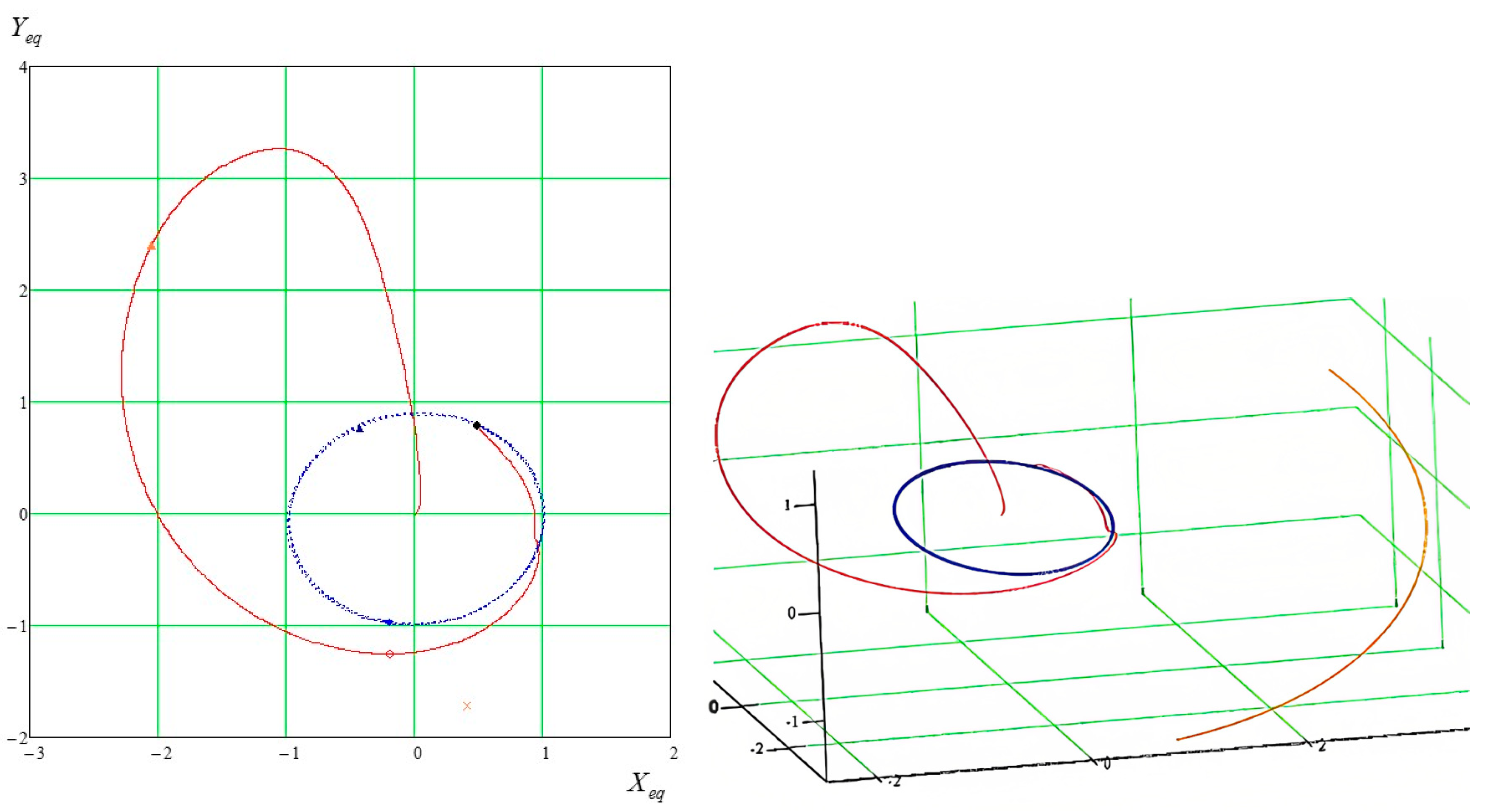
The trajectory of the SC obtained from solving the problem of the first stage; the polar angle reading direction coincides with the inertial direction of the main axis of the coordinate system ξСη(ζ), the position of which at the time of the mission start coincides with the direction to the Sun. The red solid line shows the flight trajectory; dotted blue—the Moon’s orbit; the black unfilled circle characterizes the position of the Moon at the time of launch; the black solid circle is the position of the Moon at the moment when the spacecraft reaches the given vicinity of the libration point L2; the blue diamond defines the position of the libration point; the filled orange circle describes the position of the Sun at the moments of the start of the flight and reaching the vicinity of L2, respectively.
Figure 2.
The trajectory of the SC obtained from solving the problem of the first stage; the polar angle reading direction coincides with the inertial direction of the main axis of the coordinate system ξСη(ζ), the position of which at the time of the mission start coincides with the direction to the Sun. The red solid line shows the flight trajectory; dotted blue—the Moon’s orbit; the black unfilled circle characterizes the position of the Moon at the time of launch; the black solid circle is the position of the Moon at the moment when the spacecraft reaches the given vicinity of the libration point L2; the blue diamond defines the position of the libration point; the filled orange circle describes the position of the Sun at the moments of the start of the flight and reaching the vicinity of L2, respectively.

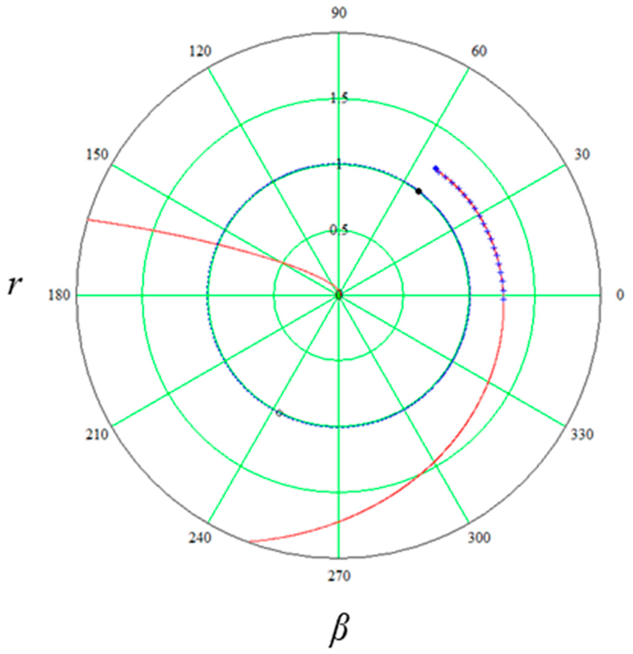
Figure 3.
The trajectory of the of the SC obtained from solving the problem of the first stage; represented in the axes of a uniformly rotating CS xCy(z).
Figure 3.
The trajectory of the of the SC obtained from solving the problem of the first stage; represented in the axes of a uniformly rotating CS xCy(z).

Figure 4.
Geocentric distance of the SC [undim.] along the flight trajectory as a function of flight time [undim.].
Figure 4.
Geocentric distance of the SC [undim.] along the flight trajectory as a function of flight time [undim.].

Figure 5.
Changing the polar angle β along the transfer trajectory as a function of flight time [undim.].
Figure 5.
Changing the polar angle β along the transfer trajectory as a function of flight time [undim.].

Figure 6.
Dependence of the perigee radius [undim.] of the osculating SC orbit as a function of flight time [undim.].
Figure 6.
Dependence of the perigee radius [undim.] of the osculating SC orbit as a function of flight time [undim.].

Figure 7.
Dependence of the apogee radius [undim.] of the osculating SC orbit as a function of flight time [undim.].
Figure 7.
Dependence of the apogee radius [undim.] of the osculating SC orbit as a function of flight time [undim.].

Figure 8.
Osculating eccentricity of the transfer orbit on the flight time [undim.].

Figure 9.
Osculating semi-major axis [undim.] of a transfer orbit on the flight time [undim.].

Figure 10.
Plane of changing the parameters “Eccentricity—semi-major axis” [undim.].

Figure 11.
Osculating argument for the perigee of a transfer orbit as a function of flight time [undim.].
Figure 11.
Osculating argument for the perigee of a transfer orbit as a function of flight time [undim.].

Figure 12.
True anomaly [deg.] as a function of flight time [undim.].

Figure 13.
Dependence of the angle between the Laplace vector of the transfer orbit and the current direction to the Sun.
Figure 13.
Dependence of the angle between the Laplace vector of the transfer orbit and the current direction to the Sun.

Figure 14.
Dependence of the change in the selenocentric energy of the spacecraft along the transfer trajectory; it is clearly seen that at the moment of approaching the SC to the vicinity of the Moon, the values of the latter pass into the negative region, thereby ensuring the possibility of realizing the spacecraft’s entry into a closed selenocentric orbit.

Figure 15.
Section of the flight trajectory with a negative value of selenocentric energy. Shown with blue crosses; it can be seen that the energy becomes negative at a fairly significant distance from the moon.
Figure 15.
Section of the flight trajectory with a negative value of selenocentric energy. Shown with blue crosses; it can be seen that the energy becomes negative at a fairly significant distance from the moon.

Figure 16.
The trajectory of the spacecraft. The solid black curve shows the section of the circumlunar motion of the SC, starting from the passage of the vicinity of the L2 point and up to the exit from the Moon’s gravity sphere through the L1 point with a further transition to the geocentric orbit.

Figure 17.
The trajectory of the spacecraft. Enlarged fragment of Figure 16.
Figure 17.
The trajectory of the spacecraft. Enlarged fragment of Figure 16.

Figure 18.
Selenocentric energy of the spacecraft [undim.] along the transfer trajectory. The blue color corresponds to the “near-lunar” section of the motion starting from time t1 to .
Figure 18.
Selenocentric energy of the spacecraft [undim.] along the transfer trajectory. The blue color corresponds to the “near-lunar” section of the motion starting from time t1 to .

Figure 19.
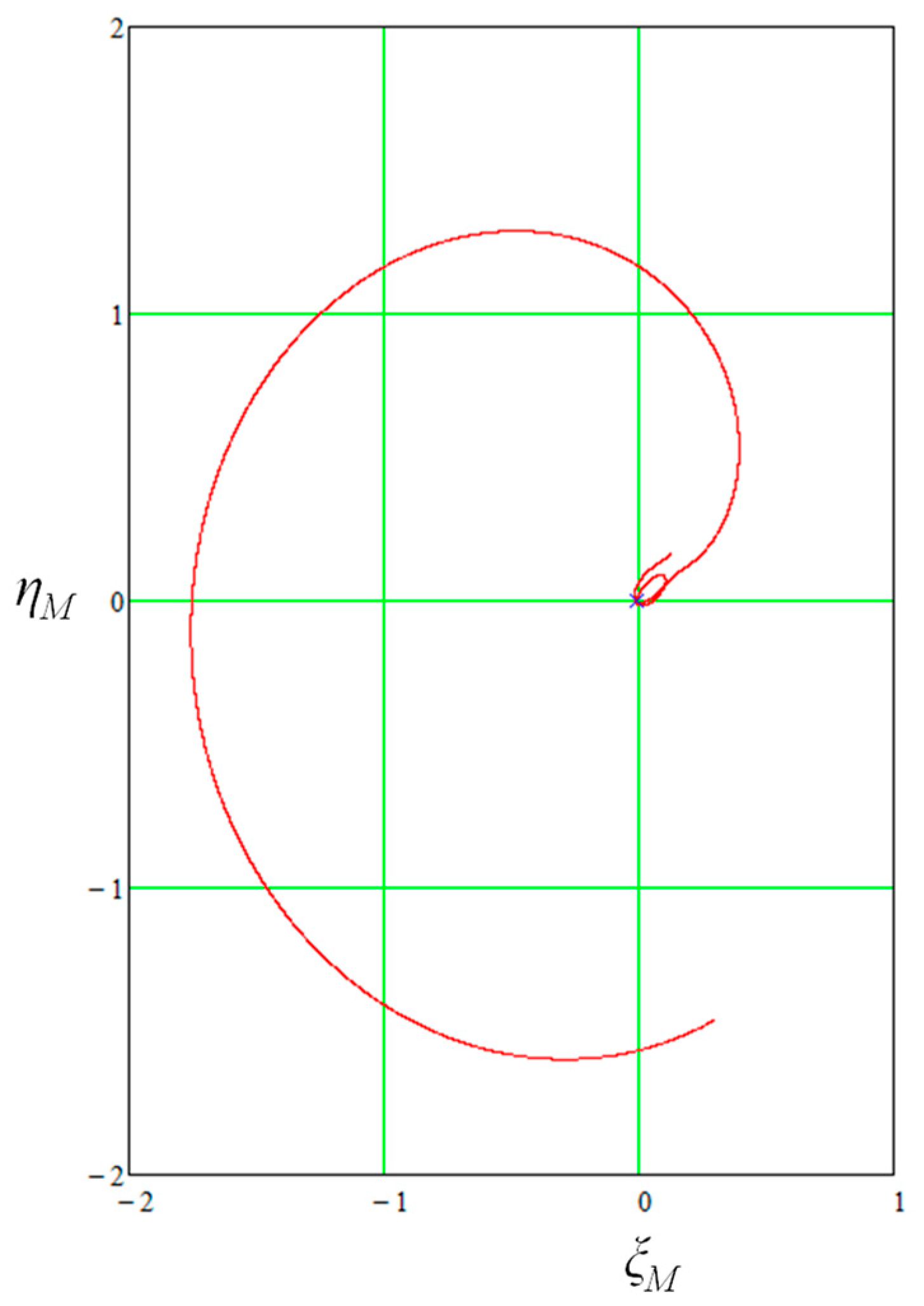
The trajectory of the spacecraft movement corresponding to the “circumlunar” segment (starting from time t1 to ). Represented in the coordinate system ξMСηM (ζ) with axes fixed in inertial space (center C coincides with the Moon) (see Appendix B), the direction of the main axis of which at the initial moment of time coincides with the direction to the Sun.
Figure 19.
The trajectory of the spacecraft movement corresponding to the “circumlunar” segment (starting from time t1 to ). Represented in the coordinate system ξMСηM (ζ) with axes fixed in inertial space (center C coincides with the Moon) (see Appendix B), the direction of the main axis of which at the initial moment of time coincides with the direction to the Sun.

Figure 20.
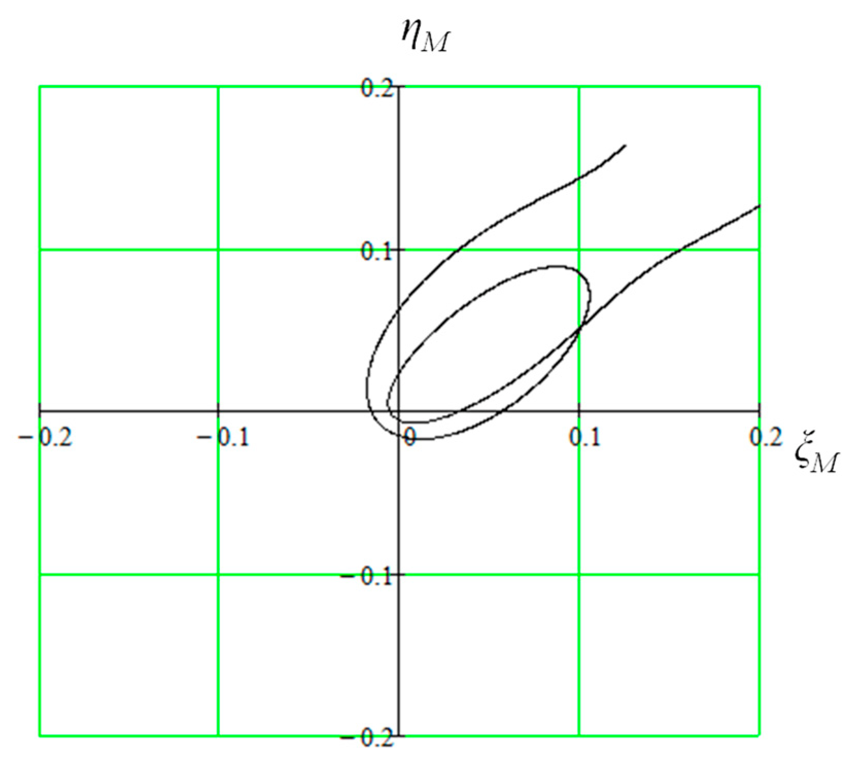
The spacecraft motion trajectory corresponding to the “circumlunar” segment (starting from time t1 to ). The shown fragment (on an enlarged scale) gives a clear idea of the rate of evolution of a closed osculating orbit.
Figure 20.
The spacecraft motion trajectory corresponding to the “circumlunar” segment (starting from time t1 to ). The shown fragment (on an enlarged scale) gives a clear idea of the rate of evolution of a closed osculating orbit.

Figure 21.
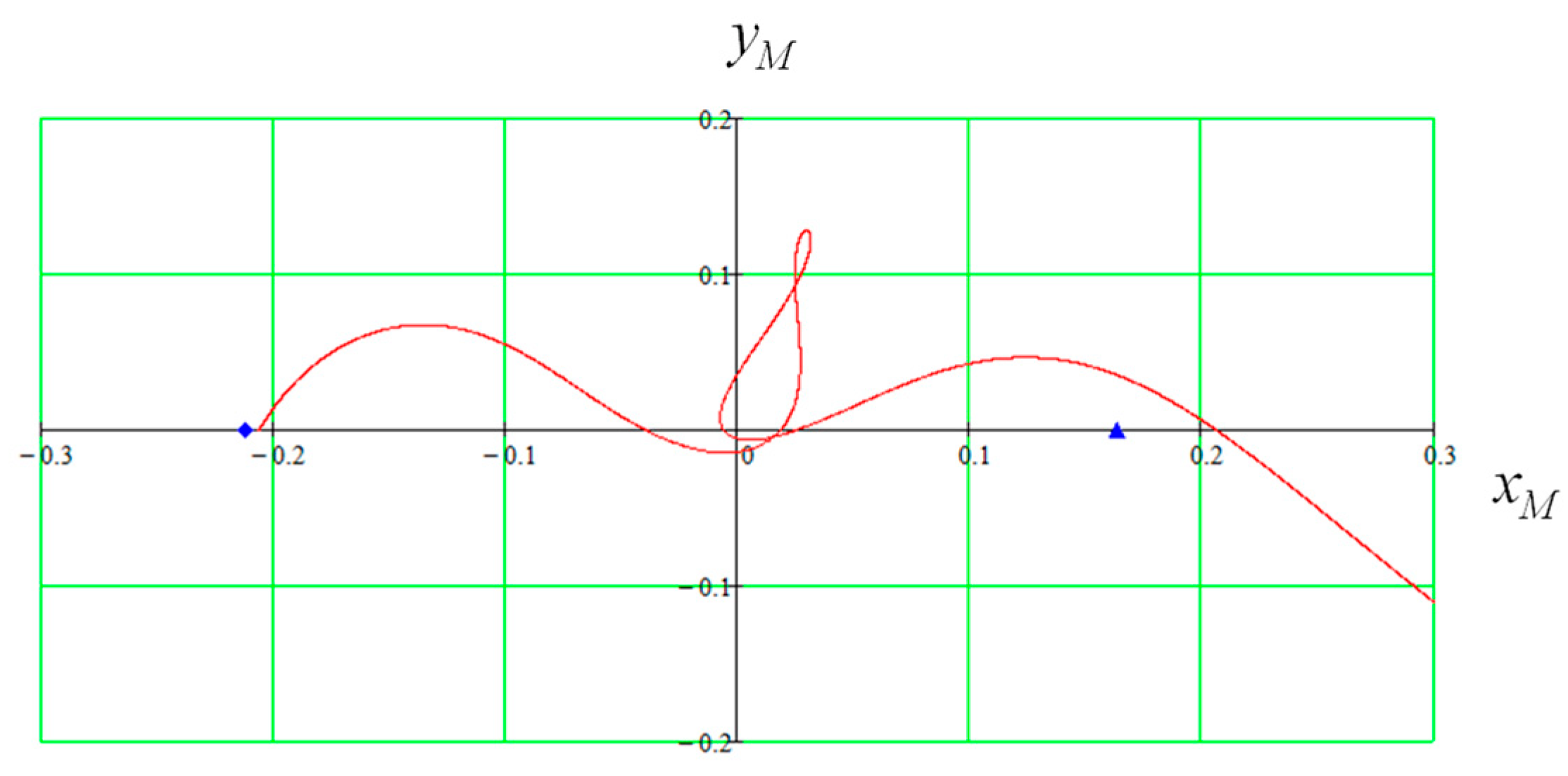
The trajectory of the SC motion corresponding to the “circumlunar” area; built in a rotating selenocentric coordinate system, the main direction of which coincides with the direction of the Moon-Earth axis. The blue rhombus shows the position of the libration point L2, the blue triangle shows the position of the point L1.
Figure 21.
The trajectory of the SC motion corresponding to the “circumlunar” area; built in a rotating selenocentric coordinate system, the main direction of which coincides with the direction of the Moon-Earth axis. The blue rhombus shows the position of the libration point L2, the blue triangle shows the position of the point L1.

Figure 22.
Complete SC trajectory starting from the moment of stratum from the Earth (black circle); built in a rotating selenocentric coordinate system, the main direction of which coincides with the direction of the Moon-Earth axis.
Figure 22.
Complete SC trajectory starting from the moment of stratum from the Earth (black circle); built in a rotating selenocentric coordinate system, the main direction of which coincides with the direction of the Moon-Earth axis.

Figure 23.
Selenocentric distance rM [undim.] along the full flight trajectory of the spacecraft. The area of “circumlunar” motion is marked in blue.
Figure 23.
Selenocentric distance rM [undim.] along the full flight trajectory of the spacecraft. The area of “circumlunar” motion is marked in blue.

Figure 24.
Relative selenocentric rM [undim.] distance between the position of the SC and the final circular orbit of a given radius.
Figure 24.
Relative selenocentric rM [undim.] distance between the position of the SC and the final circular orbit of a given radius.

Figure 25.
Relative selenocentric distance rM [undim.] of the SC to a circular orbit of a given radius (enlarged). Two points of intersection of the curve and the time axis are clearly visible, corresponding to the possible moments of entering a given circular orbit.
Figure 25.
Relative selenocentric distance rM [undim.] of the SC to a circular orbit of a given radius (enlarged). Two points of intersection of the curve and the time axis are clearly visible, corresponding to the possible moments of entering a given circular orbit.

Figure 26.
Optimal low-energy two-impulse SC flight trajectory from a 200 km low Earth reference orbit to a 100 km low selenocentric circular orbit.
Figure 26.
Optimal low-energy two-impulse SC flight trajectory from a 200 km low Earth reference orbit to a 100 km low selenocentric circular orbit.

Figure 27.
Selenocentric energy hMoon [undim.] along the optimal flight trajectory.

Figure 28.
Selenocentric rM [undim.] distance along the optimal flight trajectory.

Figure 29.
Relative selenocentric distance rM [undim.] of the SC during its trajectory motion in the “near-moon” section up to a circular orbit of a given radius.
Figure 29.
Relative selenocentric distance rM [undim.] of the SC during its trajectory motion in the “near-moon” section up to a circular orbit of a given radius.

Figure 30.
Section of the spacecraft’s selenocentric motion ending with the moment of entering the terminal orbit. The blue cross shows the point of application of the braking impulse. A fragment of the trajectory is shown in the selenocentric coordinate system with fixed axes oriented along the axes of the system ξСη(ζ) (ξMСηM(ζ)).

Figure 31.
Low-energy trajectory of the center of mass of the SC in the framework of the full model [undim.] (ICRS J2000.0).
Figure 31.
Low-energy trajectory of the center of mass of the SC in the framework of the full model [undim.] (ICRS J2000.0).


Table 1.
The optimal solution of the auxiliary problem (25).
| № | ΔV0, [km/s] | ΔV2, [km/s] | ΔVf, [km/s] | ΔVΣ, [km/s] | Start Date | Tfull, [days] |
|---|---|---|---|---|---|---|
| 1 | 3.19624 | 0 | 0.64323 | 3.83745 | 21 January 2027 | 105.348 |
Table 2.
The comparison between solutions of the main problem (bold) and the auxiliary problem.
| № | ΔV0, [km/s] | ΔVf, [km/s] | ΔVΣ, [km/s] | Tfull, [days] |
|---|---|---|---|---|
| 1 | 3.19624 | 0.64323 | 3.83745 | 105.348 |
| 2 | 3.19445 | 0.63476 | 3.82922 | 103.579 |
Disclaimer/Publisher’s Note: The statements, opinions and data contained in all publications are solely those of the individual author(s) and contributor(s) and not of MDPI and/or the editor(s). MDPI and/or the editor(s) disclaim responsibility for any injury to people or property resulting from any ideas, methods, instructions or products referred to in the content. |
© 2023 by the authors. Licensee MDPI, Basel, Switzerland. This article is an open access article distributed under the terms and conditions of the Creative Commons Attribution (CC BY) license (https://creativecommons.org/licenses/by/4.0/).
Share and Cite
MDPI and ACS Style
Nikolichev, I.; Sesyukalov, V. Design of a Low-Energy Earth-Moon Flight Trajectory Using a Planar Auxiliary Problem. Appl. Sci. 2023, 13, 1967. https://doi.org/10.3390/app13031967
AMA Style
Nikolichev I, Sesyukalov V. Design of a Low-Energy Earth-Moon Flight Trajectory Using a Planar Auxiliary Problem. Applied Sciences. 2023; 13(3):1967. https://doi.org/10.3390/app13031967
Chicago/Turabian StyleNikolichev, Ilya, and Vladimir Sesyukalov. 2023. "Design of a Low-Energy Earth-Moon Flight Trajectory Using a Planar Auxiliary Problem" Applied Sciences 13, no. 3: 1967. https://doi.org/10.3390/app13031967
Note that from the first issue of 2016, this journal uses article numbers instead of page numbers. See further details here.