Local Search Algorithm In Artificial
Overview
A local search algorithm in artificial intelligence is a type of optimization algorithm used to find the best solution to a problem by repeatedly making minor adjustments to an initial solution.
When trying to find an exact solution to a problem or when doing so would be too computationally expensive, local search algorithms come in particularly handy.
A local search algorithm in artificial intelligence works by starting with an initial solution and then making minor adjustments to it in the hopes of discovering a better one. Every time the algorithm iterates, the current solution is assessed, and a small modification to the current solution creates a new solution. The current solution is then compared to the new one, and if the new one is superior, it replaces the old one. This process keeps going until a satisfactory answer is discovered or a predetermined stopping criterion is satisfied.
Introduction
The local search algorithm in artificial intelligence is a family of optimization algorithms used to find the best possible solution to a problem by iteratively making small changes to an initial solution.
These algorithms are used to solve optimization problems in which an exact solution is either impossible to find or computationally expensive.
Hill climbing, simulated annealing, tabu search, and genetic algorithms are a few examples of different kinds of local search algorithms. Each of these algorithms operates a little bit differently, but they all follow the same fundamental procedure of iteratively creating new solutions and comparing them to the existing solution to determine whether they are superior.
The local search algorithm in artificial intelligence is a crucial tool in the field of artificial intelligence and is frequently employed to address a range of optimization issues.
Applications for local search algorithms include scheduling, routing, and resource allocation. They are particularly helpful for issues where the search space is very large and can be used to solve both discrete and continuous optimization problems.
Local Search
The nodes are expanded systematically by informed and uninformed searches in different ways:
- storing various routes in memory and
- choosing the most appropriate route,
Hence, a solution state is needed to get to the goal node. Beyond these "classical search algorithms," however, there are some "local search algorithms" that only consider the solution state required to reach the target node and disregard path cost.
In contrast to multiple paths, a local search algorithm completes its task by traversing a single current node and generally following that node's neighbors.
To solve challenging optimization issues, local search algorithms are frequently combined with other optimization methods like constraint satisfaction or linear programming. Since they can quickly converge on a solution that is close to the optimal solution, even if they do not find the exact optimal solution, they are especially helpful for problems where the search space is very large.
Q. Does a problem that is only optimized work with the local search algorithm?
The local search algorithm does indeed function for perfectly optimized problems. Any node that can provide a solution can be said to have a pure optimization problem. But the objective function's objective is to identify the best state among all of them. Unfortunately, the pure optimization problem is unable to generate excellent solutions to move from the current state to the goal state.
One of the key benefits of local search algorithms is that they can be very efficient, particularly when compared to other optimization techniques such as exhaustive search or dynamic programming. This is because local search algorithms only need to explore a relatively small portion of the entire search space, which can save a significant amount of time and computational resources.
However, one of the main limitations of local search algorithms is that they can become trapped in local optima, which are solutions that are better than all of their neighbors but are not the best possible solution overall. To overcome this limitation, many local search algorithms use various techniques such as randomization, memory, or multiple starting points to help them escape from local optima and find better solutions.
Working on a Local Search Algorithm
Local search algorithms are a type of optimization algorithm that iteratively improves the solution to a problem by making small, local changes to it. Here are the general steps of a local search algorithm:
- Initialization:
The algorithm starts with an initial solution to the problem. This solution can be generated randomly or using a heuristic. - Evaluation:
The quality of the initial solution is evaluated using an objective function. The objective function measures how good the solution is, based on the problem constraints and requirements. - Neighborhood search:
The algorithm generates neighboring solutions by making small modifications to the current solution. These modifications can be random or guided by heuristics. - Selection:
The neighboring solutions are evaluated using the objective function, and the best solution is selected as the new current solution. - Termination:
The algorithm terminates when a stopping criterion is met. This criterion can be a maximum number of iterations, a threshold value for the objective function, or a time limit. - Solution:
The final solution is the best solution found during the search process.
Local search algorithms are frequently employed in situations where it is computationally impractical or impossible to find an exact solution. The traveling salesman problem, the knapsack issue, and the graph coloring issue are a few examples of these issues.
Local Search Algorithms
A class of optimization algorithms known as local search algorithms in artificial intelligence iteratively improves a given solution by looking through its nearby solutions.
Local search algorithms' main principle is, to begin with a first solution and then move on to a better one in the neighborhood until no better solution is found. There are several types of local search algorithms, some of which are listed below:
Hill Climbing
Hill climbing is a local search algorithm in artificial intelligence applied to optimization and artificial intelligence issues. It is a heuristic search algorithm that starts with an initial solution and iteratively enhances it by making small adjustments to it, one at a time, and choosing the best adjustment that enhances the solution the most.
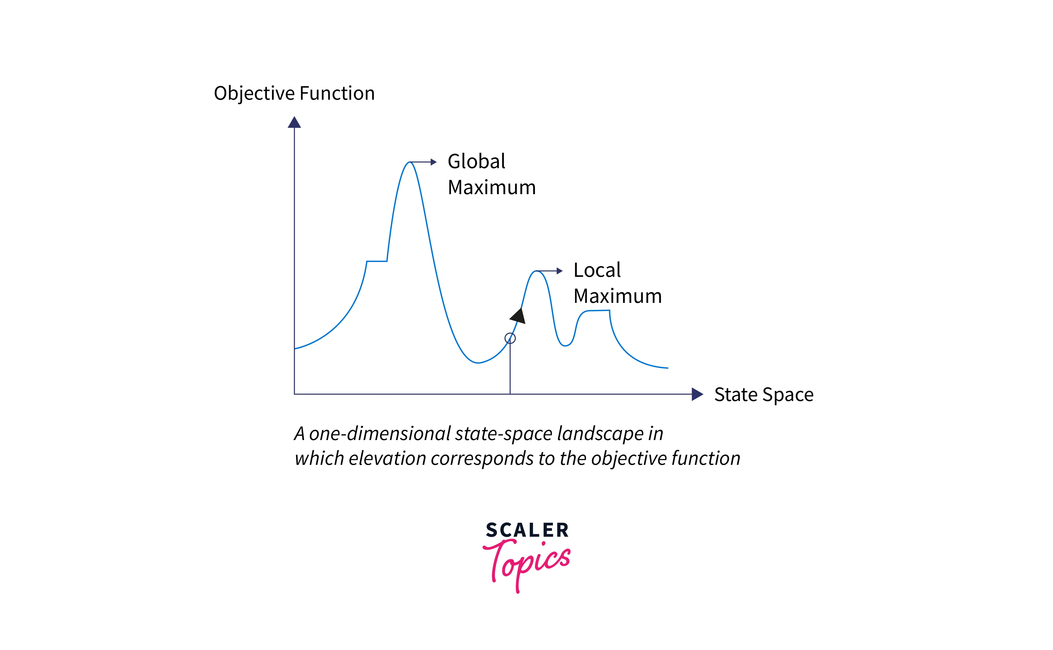
The term "hill climbing" refers to the analogous activity of ascending a hill to reach its summit (the optimal solution). The algorithm operates by making incremental progress (or "climbs") towards increasing values of the objective function up until it hits a local maximum beyond which no additional gains are possible.
The basic steps of the hill climbing algorithm are as follows:
- Start with an initial solution.
- Evaluate the objective function to determine the quality of the solution.
- Generate a set of candidate solutions by making small modifications to the current solution.
- Evaluate the objective function for each candidate solution.
- Select the candidate solution that improves the objective function the most.
- Repeat steps 3-5 until no further improvement can be made.
The simplicity and effectiveness of hill climbing, which does not require the creation and upkeep of a search tree, is one of its main benefits. Its main drawback, however, is that it might get stuck in local optima, where it is impossible to improve without first making a non-improving move. Numerous modifications to the fundamental hill climbing algorithm, including simulated annealing and tabu search, have been suggested to address this issue.
Local Beam Search
A heuristic search algorithm called local beam search is applied to optimization and artificial intelligence issues. It is a modification of the standard hill climbing algorithm in which the current states are the starting set (or "beam") of k solutions rather than a single solution.
The algorithm creates a set of candidate solutions from the current states for each iteration, evaluates those solutions, and chooses the k best ones to become the new current states.
The basic steps of the local beam search algorithm are as follows:
- Start with k randomly generated solutions.
- Evaluate the objective function for each solution.
- Generate a set of candidate solutions by making small modifications to the current states.
- Evaluate the objective function for each candidate solution.
- Select the k best candidate solutions to become the new current states.
- Repeat steps 3-5 until a stopping criterion is met.
The ability to explore multiple search paths simultaneously gives local beam search an edge over traditional hill climbing, which can increase the likelihood of discovering the global optimum. Even so, it can still find itself in local optima, especially if the search space is big or complicated.
Numerous modifications to the fundamental local beam search algorithm, including stochastic beam search and beam search with restarts, have been put forth to address this issue. With these adjustments, the search process is given a random or cyclical restart, which can aid the algorithm in leaving local optima and discovering new regions of the search space.
Simulated Annealing
Simulated Annealing is a heuristic search algorithm applied to optimization and artificial intelligence issues. By allowing the algorithm to occasionally accept moves that do not improve, this variation of the hill climbing algorithm can avoid the issue of getting stuck in local optima.
Starting with an initial solution, the algorithm iteratively generates new solutions by making minor adjustments to the original solution. The algorithm assesses the objective function of the new solution after each iteration and determines whether to accept or reject it using a probability function that depends on the difference between the values of the objective functions of the old and new solutions as well as a temperature parameter.
The basic steps of the simulated annealing algorithm are as follows:
- Start with an initial solution.
- Set the initial temperature to a high value.
- Repeat the following steps until the stopping criterion is met:
- Generate a new solution by making a small modification to the current solution.
- Evaluate the objective function of the new solution.
- If the new solution improves the objective function, accept it as the new current solution.
- If the new solution does not improve the objective function, accept it with a probability that depends on the difference between the objective function values of the current and new solutions and the current temperature.
- Decrease the temperature according to a cooling schedule.
- Return the current solution as the final solution.
The main principle of the simulated annealing algorithm is to control the level of randomness in the search process by altering the temperature parameter. High temperatures enable the algorithm to explore new regions of the search space by increasing its propensity to accept non-improving moves. The algorithm becomes more selective and concentrates on improving the solution as the temperature drops.
Simulated annealing has been successfully applied to a wide range of optimization problems, such as the traveling salesman problem, the vehicle routing problem, and the job shop scheduling problem. However, it requires careful tuning of the temperature and cooling schedule parameters to achieve good performance.
Travelling Salesman Problem
The Traveling Salesman Problem (TSP) is a well-known example of a combinatorial optimization problem in which the goal is to determine the quickest path between the starting city and a given set of cities. No known algorithm can complete it in polynomial time because it is an NP-hard problem.
Due to their capacity to efficiently search sizable solution spaces, local search algorithms in artificial intelligence are frequently used to solve the TSP. Local search algorithms for the TSP work by starting with an initial solution and incrementally improving it by making small changes to it one at a time until no more advancements are possible.

The 2-opt local search algorithm, which connects the remaining nodes in a way that minimizes the total distance, is a popular local search algorithm for the TSP. It involves removing two edges from the current solution and replacing them with two different edges. The algorithm keeps going until there is no more room for improvement.
The Lin-Kernighan algorithm, which entails a series of 2-opt moves guided by a collection of heuristics based on edge exchange and node merging, is another well-liked local search algorithm for the TSP. Although this algorithm is more complicated than 2-opt, it can produce superior outcomes.
Both 2-opt and the Lin-Kernighan algorithm are examples of local search algorithms that operate on a single solution at a time. However, to improve the chances of finding the global optimum, various modifications to these algorithms have been proposed, such as tabu search and simulated annealing. These algorithms introduce additional mechanisms to escape from local optima and explore new parts of the search space.
Conclusion
Here are the main points to conclude about local search algorithms:
- Local search algorithms iteratively improve a single solution by making small modifications to it.
- They are widely used in combinatorial optimization problems to find the best solution from a large number of possible solutions.
- Local search algorithms are often simple and efficient and can handle large solution spaces.
- However, they are prone to get stuck in local optima, where the solution is not the global optimum.
- To overcome this limitation, various modifications to local search algorithms have been proposed, such as tabu search, simulated annealing, and genetic algorithms.
- These modifications introduce additional mechanisms to explore the search space and escape from local optima but at the cost of increased complexity and computational resources.
- Local search algorithms are an important tool for solving a wide range of optimization problems and continue to be an active area of research in artificial intelligence and operations research.