Review

, Volume: 6( 3)

• View PDF
• Download PDF

3D Analytical Model of Steady Solar Faculae

*Correspondence:

Solov'ev ??, , Central astronomical observatory of Russian Academy of Science, S-Petersburg, Russia, Tel: +7 981 7170338; E-Mail: solov@gaoran.ru

Abstract

Solar facular nodes regarded as relatively stable and long-lived bright active formations with a diameter from 3 to 8 Mm and having a fine (about 1 Mm or less) magnetic filamentary structure with magnetic field strengths from 250 G to 1000 G are modeled analytically. The stationary MHD problem is solved and analytical formulae are derived that allow one to calculate the pressure, density, temperature, and Alfven Mach number in the configuration under study from the corresponding magnetic field structure. The facular node is introduced in a hydrostatic atmosphere defined by the Avrett & Loeser model and is surrounded by a weak (2G) external field corresponding to the global magnetic field intensity on the solar surface. The calculated temperature profiles of the facular node at the level of the photosphere have a characteristic shape where the temperature on the facula axis is lower than that in the surroundings but in the nearest vicinities of the axis and at the periphery of the node, the gas is 200-100 K hotter than the surroundings. Here, on the level of photosphere, the model well describes not only the central darkening of the faculae (like Wilson depression, as in sunspots), but also ring, semi-ring and segmental facular brightening observed with New Swedish 1-m Telescope at high angular resolution. In the temperature minimum region (z = 525 km), the central dip in T-profile disappears, the temperature at the facular axis considerably exceeds the temperature of the ambient plasma, and the facula as a whole is here hotter than the chromosphere. At all heights of the chromosphere the temperature of the faculae is higher than surrounding environment at the same level. This difference is particularly significant at heights of 1.5 and 2.2 Mm, where the main contribution to gas pressure within the facular node makes a pressure of the external magnetic field, which at these heights is already comparable with the internal magnetic field of the facula and even begins to surpass it. Apparently, it is these layers of the facular flux tube at heights of more than 1Mm that form the bright phenomena which are designated by observers as flocculi or plages.

Keywords

Solar facula; Photospheric-chromospheric formations

Introduction

Solar Faculae are bright areas of the photosphere that are visible in white light at the disc as well as at the limb. Although the average lifetime of elements in facular field is around 1 hour, these photospheric-chromospheric formations are actually magnetically structured and are quite entangled with the sunspots in the sense that they precede and succeed the formation of sunspots. In the Solar Dynamics Observatory (SDO/HMI) magnetograms, the facular sites are a set of small magnetic elements of different polarity, which are constantly moving, apparently under the influence of perturbations from the granules and supergranules. Against this background, however, a separate, less mobile, more stable and long-lived facular formations (facular nodes) that live up to a day or more are observed. Apparently, these objects are located at the junctions of several convection cells of supergranulation. In these cells radial-horizontal plasma flows are observed that concentrate several dozens of magnetic facular elements, which look like separate magnetic flux tubes or bundles, into intersupergranular lanes, raking them, due to the frozen-in field in the plasma, to the edges of the cells [1]. We can thereby assume that these plasma flows provide the required stabilizing effect for a prolonged existence of the facular nodes.

In this work, we will investigate specifically such relatively stable and long-lived photospheric-chromospheric magnetic formations with characteristic transverse dimensions of up to six-eight megameters with magnetic fields from 200-300 to 1000 G and having a fine internal filamentary structure on a scale of about 1 Mm or less and apparently supported by external converging boundaries of two or three nearby supergranulation cells. The gas temperature in the faculae is few hundred degrees Kelvin higher than the temperature of the surrounding chromosphere, and the temperature contrast between the individual bright elements inside the facular node does not exceed, probably, 100-200 K. At high angular resolutions (New Swedish 1-m Telescope), the facular fields in the photosphere are observed to possess a central temperature dip in the form of Wilson's depression and regular concentric segmental brightening [2,3]. Explanation of the nature of these specific temperature variations is one of the main tasks of the present model.

There are various kinds of wave and oscillatory processes that are observed in the facular fields. Roughly speaking these oscillations can be divided into two classes of different physical nature. The most studied are short-period oscillations with periods from 3-5 to 10-15 minutes [4-6]. They are usually interpreted as manifestations of acoustic and MHD waves running along magnetic flux tubes in the facula where these flux tubes play the role of resonators or waveguides. Many works have been devoted to the study of these processes, but they practically do not shed light on actual magnetic structure of a facula. Observing these wave phenomena, one can only estimate the phase velocities of the waves in order of magnitude and, accordingly, obtain the averaged order estimates of the magnetic field intensity and the plasma density. However, recently there have been reports that long-period oscillations with periods from 1 to 4 hours are observed in faculae [7,8]. These oscillations can no longer be understood within the framework of propagating MHD wave models or within the framework of the "vortex shedding" mechanism due to the stream flowing outside the faculae [9]. Apparently, they reflect the oscillations of the facula as a whole, as a single magnetic structure. In such oscillations, significant masses of gas are involved and therefore their periods are sufficiently large. These considerations already allow us to take a new approach to the problem of the structure of faculae and draw definite conclusions about their physical nature.

However, here we are not going to consider the problem of the oscillatory properties of faculae (it would require a separate study), but will concentrate only on the construction of their MHD models. One of the first physical models of the faculae was the "hot wall" model [10]. It represents the faculae as a vertical magnetic flux tube penetrating deep into the photosphere and right into the upper part of convective zone. It is assumed that the plasma density in such a tube is sharply reduced, and thus a deep Wilson depression is created which, if viewed from the side, allows us to see through the transparent tube of the facula the so called hot layers of the photosphere and the convective zone - hot walls. However, this simply overlooks the fact that when such a flux tube is observed on the limb, the observer's line of sight passes at right angles to the axis of the radially oriented facular tube, and its low layers, its hot walls, are simply not visible in this position. It turns out that, according to this model, faculae cannot be observed on the limb in principle. However, observations show the opposite picture: faculae are best seen on the limb! This lack of the model was noted in [11]. Nevertheless, observers still refer to this model: Quintero et al. [12]. Even from a theoretical point of view, the model [10] seems unsatisfactory. The expression for the transverse balance of pressures is considered to be too simple: , where B₁ is the field at the wall (12). The gas pressure in the flux tube and the density of the plasma are considered to be independent on radial distance. It will be shown below that the balance of pressures in a vertical magnetic flux tube and the density distribution in it are described by much more complicated formulae, and none of the assumptions made in Spruit (1976) are satisfied. Kostik & Khomenko, analyzing the causes of the observed brightness of facular tubes, likewise come to the conclusion that the hot-wall mechanism does not work [13], and the dissipation of MHD waves is most likely responsible for the heating of faculae. The another popular model is “hillock and cloud model” for faculae [11], which tries to describe faculae as objects not related to specific magnetic structure but possessing enhanced brightness in the vicinities of sunspots mainly due to the uplifting of hot subphotospheric plasma which is otherwise entrapped because of the large magnetic fields near the sunspot. This vertical transfer of hot subphotospheric plasma according to the authors is assumed to take place along different non-selected by any physical mechanism magnetic flux tubes and results in the formation of hot clouds which are actually observed by the observers as faculae. This model according to our opinion doesn’t represent the real nature of faculae and therefore can be mentioned for purely historical reasons.

Formulation of the problem and the governing equations

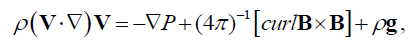
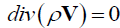
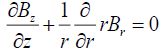
System of equations of ideal MHD in the steady case has the following form:

(1)

, (2)

, (3)

. (4)

We have used the usual notation for the various physical parameters, i.e. B is mag-netic field intensity vector, V is flow velocity vector of the fluid, P,ρ,T,μ are pres-sure, density, temperature and average molar mass of the gas respectively. The ener-gy transport equation which has a very complicated form for solar plasma is left un-determined.

The formulation of the problem requires the evaluation of stationary distributions of temperature and density which are calculable for a given magnetic structure that could answer maximally the observational properties of the modeled objects. When such a result is obtained we must explain the correspondence of the observed and theoretically predicted temperature distribution with a specific heat transfer mecha-nism in the given configuration. For example, in the case of a sunspot, all models must predict considerable low temperature of the umbra with respect to the surrounding photosphere because the strong vertical magnetic fields inhibit the convective motion of plasma in sunspots. Likewise, when the equilibrium model of the solar filaments or prominences gives the very cool plasma in their bodies, one can explain the low temperature derived from the balance of forces as a result of fast cooling of the gas due to high irradiance of dense plasma in the coronal conditions.

Most probably faculae and floccules share one and the same magnetic flux tube structure. Also it is quite possible that these structures are heated by wave dissipative processes or by joule heating mechanism. Unlike corona which has very low density and therefore very high temperature, the chromospheric structures like floccules and photospheric structures like faculae are not very hot because of corresponding high densities in comparison with corona.

Exact solutions to the problems of heat transfer and energy dissipation in active solar elements like sunspots, faculae, prominences, coronal loops and etc. are now almost impossible not only because of complicated geometry, spatial inhomogeneity and tremendous difficulty in 3D radiative transfer calculations in the continuum and in the spectral lines. We likewise have further difficulties because of our inability to reliably evaluate the contribution of MHD wave dissipation and electric current heating (Joule heating) to the energy balance of the given magnetic structure under study.

Boundary conditions of the problem: Facular nodes are studied as sufficiently solitary magnetic structures and there-fore their magnetic field at large heights and at large radial distances from the center of the facular field should attain some background value.

The demarcation boundary at the bottom of the facular structure is defined as the depth at which the average magnetic pressure in the magnetic flux tube is comparable to the dynamic pressure of convective pulsations in the photosphere:

.

At the boundary the radial profiles of pressure and temperature should have the typical form where the central region is a bit lower than the surroundings, and at large distances from the center, the profiles approach photospheric values.

Attributing a circular structure to the facular nodes, we have that at the periph-ery of this magnetic structure, the radial component of magnetic field vector ap-proaches zero and the balance of total pressures on either sides of the object is attained as it was well demonstrated in the work which studied the equilibrium of vertical magnetic flux tubes in the solar atmosphere [14]. However, as our calculations show, there is no need to attribute an abrupt sideward boundary to the facular node in our model because the described parameters steadily approach the background values as we move away from the center of the object.

Derivation of the governing equation: According to stationary ideal MHD, the plasma flow takes place along the magnetic lines of force:

, (5)

where M_A is Alfven Mach number, which is nothing but the ratio of the plasma fluid velocity and the corresponding Alfven velocity: . From the equations (2), (3) and (5) follows that:

, (6)

i.e. the factor is not change along the magnetic field line but can vary arbitrarily as we move to an another field line.

In general, the plasma flow inside the facular node possibly is small and therefore the condition (6) is satisfied sufficient ly well simply due the smallness of Alfven Mach number. Nevertheless, we still consider this parameter for the completeness of the model and this permits us to introduce the angular dependence of the field and to describe fine discrete (filamentary) structure of the field inside the node. Likewise, the external plasma flow with respect to the facular node remains subalfvenic. The super-convective converging flow is expressed in those terms where the hydrostatic pressure ex P z of the external medium at the photospheric level to which a small dynamic component 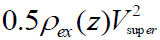is added up, where is the velocity of horizontal flow in super-granulation cells. The height profile for this velocity field is unknown and it is only possible to give an order of magnitude value: 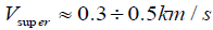. The Alfven velocity in the chromosphere with a magnetic field strength of about 10 G or more is more than 10km/s and therefore Alfven Mach number for external layers of the facular node is . The magnitude of the plasma flow velocity inside the node doesn’t exceed 1.0km / s [12].

The same estimation is quite satisfactory for polar faculae [15] and therefore we can safely assume that the flow field of gas inside these nodes is subalfvenic:

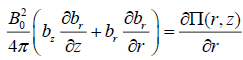
We rearrange the L.H.S of the equation (1), using the condition (5):

(7)

We use the respective vector identity and the relation (6) to get the following equation:

. (8)

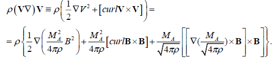
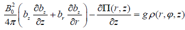
We transform the last term in the R.H.S of equation (8) using again the condition (6) to obtain the following equation for motion:

(9)

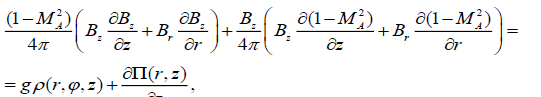
At last by representing the magnetic part of Lorenz force as , we rewrite (9) in the form [14], which constitutes the base our present research:

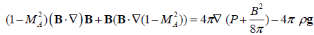(10)

The idea behind our approach is based upon the experimental observations of the long lived and stable active elements such as sunspots, faculae, chromospheric filaments and prominences, we construct the magnetic configuration of these objects up to the accuracy of few arbitrary functions and then solve the stationary MHD problem for these magnetic structures and finally obtain pressure, density and Alfven Mach number from the three components of equation (10). Later, the obtained pressure and density distributions are used in accordance with the ideal gas equation to find the respective temperature distribution. In this way for every given configuration of the magnetic field B(r) we can calculate all the required physical parameters P,ρ,T , M_A for the stationary existence of this configuration. This allows us to compare the theoretically obtained results with the observed data. The arbitrariness in the expression for the magnetic field allows us to freely choose the most relevant function that best fits the observed data. The proposed problem in the present work is similar to that which was used for modeling the sunspot [15].

Magnetic structure of steady facular configuration

We shall assume that the magnetic field of our configuration under study is not twisted i.e. the field has only two independent components but both of them are dependent on all three coordinates in the cylindrical system ( r,φ, z ):

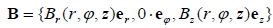. (11)

The z-axis is directed along the major axis of the cylinder and the gravitational force is represented by: . g z g e. The azimuthal component of the equilibrium equation (10) for the magnetic field given by (11), with B_{φ=0 , reduces to a following simple form:}

. (12)

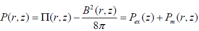
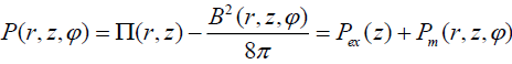
From the above expression we get the important formula for the pressure balance as:

. (13)

The function can be clearly interpreted as the total (Gas + Magnetic) pressure which doesn’t depend on the cylindrical angular coordinate but preserves the dependence on r and z. Far away from the node one has the following form:

(14)

where B_ex is the external magnetic field strength with respect to the given magnetic configuration (Obviously B_ex doesn’t depend on the size of the considered structure and also on the angle φ ). In case of small external fields we have , where is the gas pressure in the external medium. Though there is small-scale turbulence in the photosphere we can fairly assume that the external medium is hydrostatic:

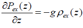(15)

The addition of small dynamic pressure ex P z and by considering (15), one obtains equation for and which can be solved by successive iterations and thereby easily correcting the hydrostatic model for the external medium. Calculations demonstrate that the above corrections are quite small i.e. they are small by two orders of magnitude with respect to the initial values. Therefore we can restrict ourselves to the addition of the small term which can be solved by successive iterations and thereby easily correcting the hydrostatic model for the external medium. Calculations demonstrate that the above corrections are quite small i.e. they are small by two orders of magnitude with respect to the initial values. Therefore we can restrict ourselves to the addition of the small term to the hydrostatic profile at small photospheric heights.

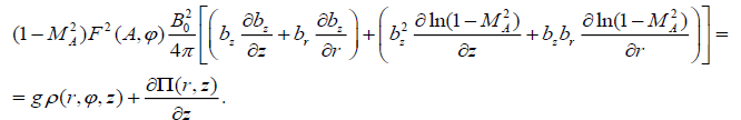
We now write down equations for two other components in the equation (10) by substituting expression (13) in the R.H.S.

(16)

. (17)

Now we determine the components of the magnetic field with the help of the magnetic flow function. Simplifying equation (3) in terms of cylindrical coordinates, we get:

. (18)

It follows that the longitudinal and radial fields must be expressed in terms of the function and some arbitrary dimensionless function of the magnetic flow and the angular coordinate F(A,φ) :

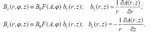(19)

B₀ is taken as the unit for the measurement of magnetic field strength. By a simple substitution of these expressions in (18), one can see that the magnetic field given by (19) is conditionally solenoidal for any arbitrary differentiable function F(A, φ) . The dependence of the function F on the angular coordinate can be arbitrarily defined, for example in such a simple type:

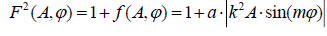. (20)

where F(A, φ) is the positive oscillating component with decreasing amplitude as we move above in height because of decreasing magnetic flow A. In (20) a, m are some positive coefficients, k= (1Mm)^-1 is the reciprocal height scale which was introduced to rewrite equation (20) in a dimensionless form. The large values of m allow us to describe fine discrete structure inside the facular node due to the combination of radial and angular dependence in equation (20) (FIG. 1). In particular, the circular and semicircular structures can be described which are usually observed in the facular fields at high angular resolutions [2].

If there is no angular dependence, than F = 1.

By substituting expression (19) in the formulas (16) and (17) we get:

(21)

(22)

The R.H.S. of the expression (21) doesn’t contain the angular dependence. Consequently, we must take:

(23)

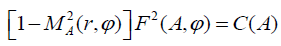
where С(А) is some positive function of the magnetic flow which is independent of the angular coordinate. In this case, the expression

depends on A and φ only, and therefore the small logarithmic terms in the second round brackets of the L.H.S. of the equations (21) and (22) identically equal to zero due to Equation (19). One of the cofactors in the L.H.S. of (23) is less than unity and the other is oscillatory above one. Considering that the function F is chosen sufficiently arbitrarily one can take C = 1 for the simplification of the model which then leads to the following:

. (24)

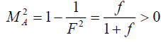
In the limiting case when , one has . As f approaches to1, we get and if we have . If we take , 1, then in all the formulas below we must use the product CB₀ instead of B₀. In principle, this will not affect the results of the model, only the numerical estimates of the magnetic field intensity in the faculae will slightly change. For example, we should use 1100 or 900 G instead of 1000G.

In this way equations (21), (22) take the form:

, (25)

. (26)

The L.H.S. of the equation (26) doesn’t depend on the angle, consequently this dependence disappears for the distribution of plasma density which in our configuration happens to have an axially symmetric form: ρ = ρ (r, z) .

The expression (25) with the help of (14) is integrated with respect to r from some point of the node to an another point infinitely distant from the node:

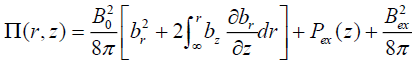. (27)

Substituting in (25) we get:

. (28)

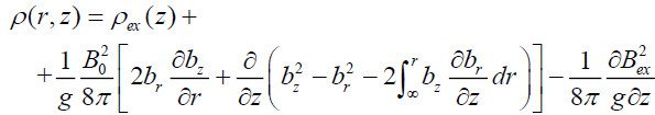
The balance of pressures given by (27) with axial symmetry can be rewritten as:

, (29)

where 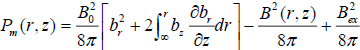represents the deviation of gas pressure in the node from the corresponding hydrostatic distribution due to the magnetic field. Analogously the expression for the density of gas can be written as:

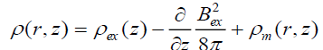, (30)

where 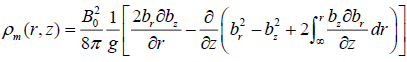is the deviation of density from the corresponding hydrostatic distribution owing to the presence of the magnetic field in the node.

For the asymmetric case the equation (30) is unchanged as the density distribution doesn’t have azimuthal dependence but we obtain a dependence on angle in the equation (29) because of the following term B²(r, z,φ) :

(31)

where 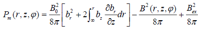is dependent on the angle corresponding to the additional magnetic component B²(r, z,φ) .

In the obtained formulas the important uncertainty is constituted by the term containing and the derivative of it with respect to height. To consider these, we must introduce an extra hypothesis. We are going to consider the simplest possible form: B_ex = const =2G, which corresponds to the global magnetic field strength at the level of the photosphere. This field varies with height by the scale of hundreds of thousands of km. At the scale of chromospheres i.e. about 2Мm [16], which is considered here, these changes are negligibly small and the expression for the density of the gas (30) can be considered free of the small term .

The expressions (29), (30), (31) with the known functions allow us to calculate the distributions of gas pressure and gas density in the stationary facular node. As one can notice, the exact evaluation of the magnetic force gives the equation which is considerably complex in comparison to the usually used simple equation of pressure balance 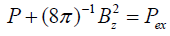which is true only in the absence of the radial field, gas flow and angular dependence.

We underline that by the substitution of the potential magnetic field in (30), the function , one immediately obtains zero. At the same time the zero of the function demands in the correspondence with the physical meaning, the absence of plasma flow demands in the correspondence with the physical meaning, the absence of plasma flow and the azimuthal variation of the field . This test serves as means of check to the correctness of all the carried out calculations.

The structure of the magnetic field in the facular node

To describe the magnetic structure of the node, we use as an initial approximation the following solution obtained by Schatzman (1965) in its potential limit:

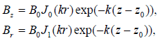(31)

The above distributions are obtained from the following magnetic flow function

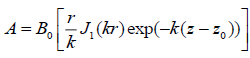. (32)

Here 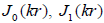are the Bessel functions of zeroth and first orders, B₀ is the magnetic field strength at the level of the 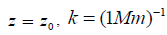is the reciprocal height scale. After the substitution of the expression for potential magnetic field (31) in the obtained formulae for the gas pressure and gas density, one naturally gets unperturbed background values as the magnetic force of the potential field is zero. To get the non-potential force configuration, it is needed to introduce the respective corrections into the magnetic structure (31). We introduce two needed corrections into our model as follows: (i) angular dependence given by the function F (see formula (20) and FIG. 1), and (ii) the substitution of the exponents in (31) by the expression:

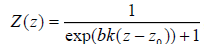, (33)

This expression describes a distorted step (well known in quantum mechanics as the Fermi-Dirac distribution): the positive coefficient b defines the order of distortion of the step, larger values of b lead to abrupt edge of the step. Here is some level of the coordinate system where the step is reduced to one half, and therefore in the case we should take into account that B₀ in the formula (31) will be different from B(0) , i.e. from the magnetic field strength at the starting level 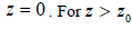this function approaches to exp(-bkz), and therefore for the magnetic field to approach a potential form at large heights, we must introduce the same coefficient b in the argument of the Bessel functions (31).Then the magnetic field flow with new variables takes the following form: 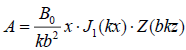, where x =br , and the components of the field are expressed as: , where the derivative is taken over the argument bkz. For , , the magnetic field in the flux tube which goes down stops to be dependent on the depth (FIG. 2). For the calculations, we will take z₀ = 0.125Mm, and the level of the photosphere is considered as the level with z = 0 . For this case: B(0)= 0.62246  B₀ . In accordance with the model Avrett & Loeser (2008), at the level of the photosphere the plasma parameters are:

.

The angular parameter m (together with the radial parameter b) determines the number of elements of the fine structure of the magnetic field in the facular unit. Observations show that this number for a large node is from several units to several tens. We took m = 7, which gives, as can be seen from FIG. 1, 42 elements of a fine structure for a node with a diameter of 5Mm. This choice of m seems to us quite acceptable. Of course, another choice of this parameter is possible; this has no effect on other properties of the model.

The magnetic field of the faculae described by the formula (31) has a multipolar character with a strong vertical field at the center. However, observers claim that the magnetic field of the faculae is unipolar (single polarity structure) [12,15]. The fact is that in any magnetic field observations, one observes not the magnetic field strength at a particular point but have an averaged value over some surface around this point . In the present model under overall averaging of the longitudinal component of the field over an arbitrary circular area, we get: . This function shown in FIG. 3, has a strong central maximum and the magnitude of the of negative maximum is 13.5%. The negative polarity occupies narrow ring zone. Even on the magnetograms which are obtained from Solar Dynamics Observatory by the instrument HMI, with a characteristic noise level of 10-15% [7,17] the narrow zone with the opposite polarity will be faint and the observers find the faculae as single polarity structure. This is all the more true for ground-based observations.

After the substitution of corrected expression for (31) in (30), we obtain for the pressure in the node, the following expression:

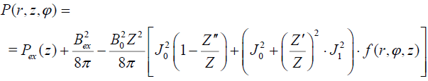(34)

where . In this formula the sign of the first term of the added magnetic component to the gas pressure is always positive: for the second derivative is smaller than Z and rapidly vanishes. For , we have and for the difference approaches to zero. The second term in square brackets of (34) contains the angular coordinate and together with the radially varying Bessel functions gives discrete structure to faculae. This second term tends to zero, at large heights and at large radial distances.

For the density, the formula analogously has the following form:

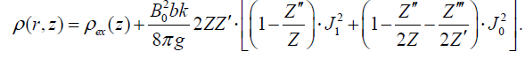(35)

Here the dash over Z indicates the derivative with respect to the argument of the exponent (bkz). In case of potential field (31) i.e. when the function Z is expressed by the exponent, 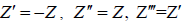, and the expression in the square brackets equals to zero. When the function Z(z) is given by the formula (33), the value of this bracket is different from zero at small heights and tends to zero for large heights. With the increase in the radial distance the value of the bracket likewise tends to zero due to the diminishing Bessel functions.

Calculations and Discussions

Here we are going to show numerical calculations of temperature distributions in the node obtained from the formulae (33), (30), (4) and with the help of solar atmospheric model [16]. These distributions will be calculated at the level of photosphere (z = 0 km), temperature minimum (z = 525km), and similarly at heights of about z = 1032km , z = 1520 km and z = 2083km.We have considered the following parameters for the function Z: b = 4, z₀ = 0.125Mm . For the angular part, we considered m = 7 . Finally for the magnetic field strength in the facular node at photosphere, we take two values: B(0) =1000G and B(0) = 500G, for the photosphere we had to consider an additional case B(0) = 250G.

As can be seen from FIG. 4 and 5, the temperature profiles of the faculae completely conserves their geometrical form under a changing magnetic field strength but when the field strength reduces from 1000 to 250 G there is a respective reduction in the temperature range of the faculae: if for B(0) =1000G this range is about 1500К, then for B(0) = 250Git reduces to around 25 times less. Consequently, we observe the following variation of temperature between successive elements of the faculae, in the first case a variation is about two hundreds of Kelvin and in the second case it is of two tens of Kelvin.

In all cases at the level of photosphere there is a central fall in temperature (similar to the Wilson’s depression in sunspots), but a faculae as a whole is hotter than the surrounding photosphere and therefore is clearly visible on the background of the photosphere.

These profiles quite interestingly are similar to usual torches that we use in the day to day life. They resemble a bright source with a handle which is used to hold the torch.

Level of the temperature minimum, z = 525км. The temperature of chromosphere is 4410К

Here the temperature along the axis of faculae doesn’t decrease. The faculae as a whole are situated above the background and should be observed clearly from this height, the variation in temperature between lower and upper regions of the profile is about of 1400 K at the case B(0) =1000G. We once again see that the geometrical form of the temperature profile doesn’t change for large changes of the corresponding magnetic field strength, here only the temperature range changes (FIG. 6).

Level of z = 1032км, the temperature of chromosphere is 6315К

Here the temperature is large enough at the narrow central region of the faculae but the main body and periphery are slightly hotter than the surroundings ( FIG. 7).

Level with z = 1520 km, the temperature of chromosphere is 6623К, the gas pressure is 1.133 dyn/cm²

At these levels in the central region of the faculae, the temperature is very high and the faculae as a whole appears to be more hotter than the surroundings. Here the yellow plane doesn’t represent the temperature of background that is 2000K lower than the average temperature of the facula. This plane represents only the temperature of the lowest layer of the faculae. Here the angular variation of the field doesn’t play a noticeable role (FIG. 8).

Level near the transition region, z =2083 km, the temperature of the chromosphere is 7729 K (FIG. 9)

As one approaches the transition region, the temperature of the faculae markedly increases due to the constant
pressure of external magnetic field: .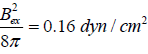

Conclusions

1. A steady MHD model for the solar facular node with fine filamentary structure of the magnetic field and the temperature is constructed. Analytical formulae for the calculation of gas pressure, density, Alfven Mach number and temperature according to the given magnetic configuration are obtained.

2. Facular magnetic configuration with external magnetic field of 2G is introduced for the solar atmosphere which is described by the modern empirical model Avrett & Loeser (2008).

3. Numerically evaluated profiles of plasma temperature inside the facular node at the level of the photosphere have the following form: there is negative contrast at the axis (Wilson’s depression), but at the nearest vicinities the temperature sharply rises and local rise in temperature of the individual facular granules above the surrounding medium is observed all along the area of the faculae. The geometry of profiles doesn’t change even for large magnetic field variations. The variation of magnetic field only results in the change of the temperature range in the faculae.

4. At the height of the temperature minimum (525 км), the central temperature dip disappears and the entire profile of the faculae is located above the background and has temperature one and a half times more that of the ambient plasma at this level.

5. At the heights of 1500-2000 km above the photosphere, the gas of faculae is two and half times hotter than the ambient plasma at the same level.

6. Most likely that due to the fact that faculae have a high temperature at the heights above 1 Mm, the observers distinguish between faculae and flocculi as two different phenomena. Faculae are considered to be photospheric and lower chromospheric phenomena and flocculi or plages are considered to be the upper chromospheric phenomena[18,19].

7. In whole, the parameters and of the proposed model are in good correspondence with the most recent observational data of the solar faculae. This model in particular firstly describes periodic concentric rings, half rings and segmental brightening observed in the facular fields at high angular resolution at the photosphere [2,3].

Aknowledgement

The work was supported by the Russian Foundation of Basic Researches (project № 18-02-00168) and Russian Science Foundation (project 15-12-20001).

References

1. Аvrett EH, Loeser R. Models of the Solar Chromosphere and Transition Region from Sumer and HRTS Observations: Formation of the Extreme-Ultraviolet Spectrum of Hydrogen, Carbon and Oxygen. The Astrophy J Suppl Ser. 2008;175:229-76.
2. Baltasar H. The oscillatory behavior of solar faculae. Solar Phys. 1990;127: 289-92.
3. Berger TE, Rouppe L, Lofdahl M. Contrast analysis of solar faculae and magnetic bright points. The Astrophys J. 2007;661:1272-88.
4. Chelpanov AA, Kobanov NI, Kolobov DY. Astron Rep.2015; 59:96.
5. Kolotkov D Y, Smirnova V V, Strekalova PV, et al. Long-period quasi-periodic oscillations of a small-scale magnetic structure on the Sun, Astron Astrophys. 2017;598:4.
6. Kostik R, Khomenko E. The possible origin of facular brightness in the solar atmosphere. Astron Astrophys. 2016;589:A6.
7. Lites BW, Scharmer GB, Berger TE, et al. Three-dimensional structure of the active region photosphere as revealed by high angular resolution. Solar Phys. 2004;221:65-84.
8. Mehltretter JP. Observations of photospheric faculae at the center of the solar disk. Solar Phys. 1974;38:43-57.
9. Nakariakov VM, Aschwanden MJ, van Doorsselaere T. The possible role of vortex shedding in the excitation of kink-mode oscillations in the solar corona. Astron Astrophys. 2009;502:661-4.
10. Okunev OV, Kneer F. On the structure of polar faculae on the Sun. Astron Astrophys. 2004;425: 321-31.
11. Quintero Noda C, Suematsu Y, Cobo Ruiz B, et al. Analysis of spatially deconvolved polar faculaeMon Not R Astron Soc. 2016;460:956–65.
12. Shatten KH, Mayr HG, Omidrav K, et al. A hillock and cloud model for faculae.The Astrophys J. 1986;311:460-73.
13. Schatzman E. Model of a force free field. IAU Symp. 22, Stellar and solar magnetic fields. Amsterdam. 1965:337-345.
14. Scherrer PH, Shou J, Bush RI et al. The Helioseismic and Magnetic Imager (HMI) Investigation for the Solar Dynamics Observatory (SDO). Solar Physics. 2012;275:207-27.
15. Solov’ev AA., Kirichek EA. Analytical Model of an asymmetric sunspot with a steady plasma flow in its penumbra. Solar Physics. 2016;291:1647-63.
16. Solov’evA. A., Kirichek E.A., Magnetohydrostatics of a vertical flux tube in the solar atmosphere: coronal loops, a model of a ring flare filament. Astron Lett. 2015;41:211-24.
17. Spruit HC. Pressure equilibrium and energy balance of small photospheric flux tubes. Solar Phys. 1976;50:269-95.
18. Strekalova PV, Nagovitsyn YA, Riehokainen A, et al. Long-period variations in the magnetic field of small-scale solar structures. Geomagn Aeron. 2016;56:1052-9.
19. Thomas JH, Cram LE, Nye AH. Dynamical phenomena in sunspots. I-Observing procedures and oscillatory phenomena. II-A moving magnetic feature. Astrophys J. 1984;285:368-85.